Multivariate statistical process control methods for batch production: a review focused on applications

ABSTRACT

In this paper, we highlight the basic techniques of multivariate statistical process control (MSPC) under the dimensionality criteria, such as Multiway Principal Component Analysis, Multiway Partial Squares, Structuration à Trois Indices de la Statistique, Tucker3, Parallel Factors, Multiway Independent Component Analysis, Multiset Canonical Correlation Analysis, Slow Features Analysis, and Parallel Coordinates. Furthermore, we summarize the procedures of each statistical technique and the usage of multivariate control charts. In addition, we review the most significant proposals and applications in practical cases. Finally, we compare and discuss the benefits and limitations within methods.

KEYWORDS:

• MSPC
• batch
• methods
• review
• applications

1. Introduction

Multivariate statistical process control focuses on process monitoring in which several related variables are involved (Bersimis et al., 2007). Nowadays, there are many industrial scenarios where simultaneous monitoring or control of two or more related quality–process characteristics is necessary. In particular cases, several industries rely on batch processing, including, for example, chemicals, pharmaceuticals, food products, fabrics, metals, bakeries, pulp, and paper manufacturers. In this specific situation, high-quality products are commonly described by quality characteristics (variables), each of which must be controlled within specifications to maintain customer satisfaction and to describe the process performance as the batch progresses (Lewis, 2014).

Pioneer work on multivariate process control was first illustrated in an air testing of sample bombsights case (Hotelling, 1947). This key point gave way too many other techniques, such as multivariate extensions for all kinds of univariate control procedures and control charts like multivariate Shewhart-type, cumulative multivariate sum (MCUSUM) and multivariate exponentially weighted moving average sum (MEWMA) (Bersimis et al., 2007). However, these procedures only took into consideration the multivariate approach, leaving behind further considerations where independence and multinormality are not always verifiable.

In batch processes, traditional multivariate procedures became unusable and principal contributions appeared with multivariate projection methods. As for our concern, first novel approaches to batch monitoring were mostly grounded on multiway partial least squares (MPLS) and multiway principal component analysis (MPCA) (Nomikos & MacGregor, 1994, 1995a). From that moment on, several strategies and methods have been developed in order to meet statistical assumptions, such as correlation-autocorrelation structure, distribution and parameter free, non-linearity, among others, typical in batch production models (Lewis, 2014).

As known, multivariate process control is one of the most rapidly developing areas of statistical process control and the need for review papers is increasingly compelling for boosting new research ideas in batch processing (Bersimis et al., 2007; Woodall & Montgomery, 1999). This paper is the result of a literature review of the most recent developments in the area of multivariate statistical process control, considering batches datasets.

The remaining sections are organized as follows. A brief review of the article search methodology is detailed in Section 2. The standard terminology used throughout the paper is specified at the beginning of Section 3. Dimensionality and non-dimensionality reduction methods are described in Sections 3.1 and 3.2, respectively. Relevant proposals and applications of these strategies are summarized in Section 4. Finally, some concluding remarks are delivered in Section 5.

2. Materials & methods

Scholar Google and Databases were searched for relevant articles using the keywords ‘MSPC’, ‘batch’, ‘application’, and ‘review’ from 1990 to 2018. As a result, about 160 articles were searched and reviewed. Only 37 publications from 23 journals and 9 databases were selected from the previous search and analyzed in detail, focused on the criteria of practical applications in industrial processes. Articles with application on matrices instead of multiway arrays were less considered. The databases distribution of articles can be observed in Table 1.

Table 1. Distribution of reviewed articles based on databases

Databases	Articles
Science Direct	11
Wiley Online Library	6
ACS Publications	6
Taylor & Francis Online	5
IEEE Xplore	5
Springer	1
Others	3

3. Multivariate statistical process control (MSPC) for batches datasets

When it comes to batches, is common to find datasets as tensors or multilinear arrays, typically, three-way arrays $\left[\mathbf{X}\right]$ with data collected from $I$ batches, $J$ variables, and $K$ observations as shown in Figure 1 (Bersimis et al., 2007).

Figure 1. Three-way array dataset

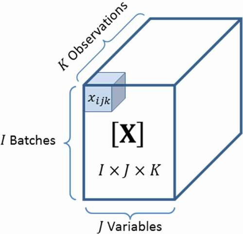
In some cases, the third way is not a ‘$K$’ number of observations, instead, an ordered time succession is considered.

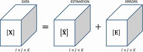
A wide variety of methods are used to control batches in MSPC. Most of them rely on dimensionality reduction via decomposition of the multilinear array $\left[\mathbf{X}\right]$ (Figure 2) considering lower rank approximation to represent it, ending with an estimated array $\left[\hat{\mathbf{X}}\right]$ and its corresponding errors tensor $\left[\mathbf{E}\right]$ that can be obtained as $\left[\mathbf{E}\right]=\left[\mathbf{X}\right]-\left[\hat{\mathbf{X}}\right].$

Figure 2. Errors from estimation in dimensionality reduction

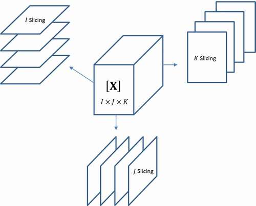
An unfolding procedure of the three-way array is performed in several methods. Three different slicing perspectives (Figure 3) are possible within this context:

• $I$-slicing delivers $J\times K$tables ${\mathbf{X}}_i^{\left(I\right)}$ or $K\times J$tables ${\left({\mathbf{X}}_i^{\left(I\right)}\right)}^{\mathrm{T}}$ for every batch

• $J$- slicing delivers $I\times K$tables ${\mathbf{X}}_j^{\left(J\right)}$ or $K\times I$tables ${\left({\mathbf{X}}_j^{\left(J\right)}\right)}^{\mathrm{T}}$ for every variable

• $K$- slicing delivers $I\times J$tables ${\mathbf{X}}_k^{\left(K\right)}$ or $J\times I$tables ${\left({\mathbf{X}}_k^{\left(K\right)}\right)}^{\mathrm{T}}$ for every observation.

Figure 3. Slicing perspectives in three-way arrays

Then, according to the subject of the study 12 types of unfolding can be done, as shown in Table 2:

Table 2. Different unfolding perspectives for a three-way array

Slicing dimension	Rightwards One next to the other		Downwards One below to the other
	Matrix	Order	Matrix	Order
$I$	${\mathbf{X}}^{\left(I_R\right)}$	J$\times IK$	${\mathbf{X}}^{\left(I_D\right)}$	$IJ\times K$
$J$	${\mathbf{X}}^{\left(J_R\right)}$	$I\times JK$	${\mathbf{X}}^{\left(J_D\right)}$	$IJ\times K$
$K$	${\mathbf{X}}^{\left(K_R\right)}$	$I\times JK$	${\mathbf{X}}^{\left(K_D\right)}$	$IK\times J$
Slices transposed
$I$	${\mathbf{X}}^{{\left(I_R\right)}^{\mathrm{T}}}$	$K\times IJ$	${\mathbf{X}}^{{\left(I_D\right)}^{\mathrm{T}}}$	$IK\times J$
$J$	${\mathbf{X}}^{{\left(J_R\right)}^{\mathrm{T}}}$	$K\times IJ$	${\mathbf{X}}^{{\left(J_D\right)}^{\mathrm{T}}}$	$JK\times I$
$K$	${\mathbf{X}}^{{\left(K_R\right)}^{\mathrm{T}}}$	$J\times IK$	${\mathbf{X}}^{{\left(K_D\right)}^{\mathrm{T}}}$	$JK\times I$

For simplicity purposes, in this review we are going to consider the following notation:

$K$-slices are $I\times J$ tables ${\mathbf{X}}_k^{\left(K\right)}$, and $K$-unfold displays the $I\times JK$ table ${\mathbf{X}}^{\left(K\right)}$, while $J$-unfold displays the $IK\times J$ table ${\mathbf{X}}^{\left(J\right)}$; also, $I$-slices are $K\times J$ tables ${\mathbf{X}}_i^{\left(I\right)}$, and $I$-unfold displays the $K\times IJ$ table ${\mathbf{X}}^{\left(I\right)}$.

After the unfolding step, the application of singular value decomposition (SVD) is usual, where two or more principal components are subject of main analysis using the Hoteling’s $T^2$ statistic, or similar, like $D^2$ statistic. Errors block is also monitored with statistics, such as Q and SPE. Two principal components allow to generate practical visual approaches, nevertheless, for $T^2$ control charts, cross-validation can be applied to define an optimum $R$ number of components to use.

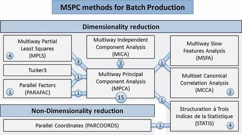
Based on the literature reviewed during this study, two main groups of multivariate statistical methods can be discerned: those that reduce dimensionality and others that preserve data original dimension.

According to the presented classification of MSPC methods for batch production, the reviewed articles were distributed as shown in Figure 4. It is important to point out that some of these articles consider two or more methods to compare their performance and highlight a specific one, under predefined criteria.

Figure 4. Schematic overview of MSPC methods and articles’ distribution by dimensionality criteria

3.1. Dimensionality reduction

3.1.1. Multiway principal component analysis (MPCA)

MPCA was first proposed by Wold et al. (1987), and later Nomikos and MacGregor (Nomikos & MacGregor, 1994) suggested a formal methodology for batch processes. This method allows a reliable feature extraction of the data and projection onto a sub-space of fewer dimension, easier for graphing and interpretation (Lu et al., 2008).

From a given multiway array $\left[\mathbf{X}\right]$ of reference batches, MPCA performs $K$-unfolding (Figure 5) and column centering, then conventional PCA is applied (Abdi & Williams, 2010). The preprocessed matrix ${\mathbf{X}}^{\left(K\right)}$ exhibits the following PCA decomposition:

${\mathbf{X}}^{\left(K\right)}=\mathbf{P}{\mathbf{Q}}^{\mathrm{T}},\hspace{0.17em}{\mathbf{Q}}^{\mathrm{T}}\mathbf{Q}=\mathbf{I}$

$x_{i\left(jk\right)}=\sum _{r=1}^R{p}_{ir}{q}_{\left(jk\right)r},\left(jk\right)=\left(k-1\right)J+j$

Figure 5. K-unfolding and MPCA method scheme

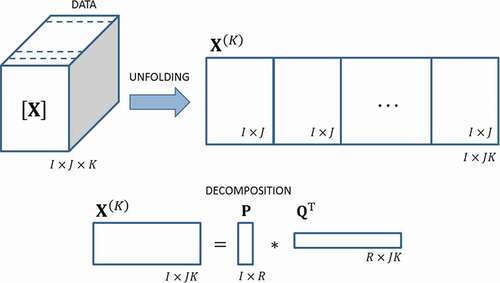
Scores ($\mathbf{P}$) and loadings ($\mathbf{Q}$) are obtained. The common practice is to use scores in a biplot (t₁-t₂ scores plot), which involves $R$ retained components, typically the first and second ones (Macgregor, 1997). Also, projected data into the t₁- t₂ scores plot help to define confidence regions (Geladi et al., 2003).

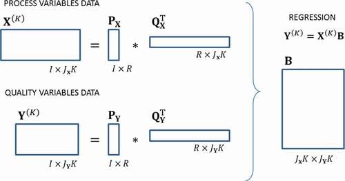
3.1.2. Multiway partial least squares (MPLS)

PLS is also referenced as Projection to Latent Structures because the method’s purpose is to obtain a reduced representation of the main information, using latent variables. It is based on the strong correlation between process and quality variables sets, $\mathbf{X}$ and $\mathbf{Y}$ respectively (Nomikos & MacGregor, 1995a).

MPLS performs very well when enough historical data are available, allowing to draw inferences (Flores-Cerrillo & MacGregor, 2005). As in MPCA takes place, the tensors for process variables $\left[\mathbf{X}\right]$ and quality variables $\left[\mathbf{Y}\right]$ must be $K$-unfolded into two-way matrices and then, PLS steps are applied (Abdi, 2010). The decomposition of preprocessed matrices ${\mathbf{X}}^{\left(K\right)}$ and ${\mathbf{Y}}^{\left(K\right)}$ is done as follows:

${\mathbf{X}}^{\left(K\right)}={\mathbf{P}}_{\mathbf{X}}{\mathbf{Q}}_{\mathbf{X}}^{\mathrm{T}},{\mathbf{Q}}_{\mathbf{X}}^{\mathrm{T}}{\mathbf{Q}}_{\mathbf{X}}=\mathbf{I}$

${\mathbf{Y}}^{\left(K\right)}={\mathbf{P}}_{\mathbf{Y}}{\mathbf{Q}}_{\mathbf{Y}}^{\mathrm{T}},{\mathbf{Q}}_{\mathbf{Y}}^{\mathrm{T}}{\mathbf{Q}}_{\mathbf{Y}}=\mathbf{I}$

Scores (${\mathbf{P}}_{\mathbf{X}},\hspace{0.17em}{\mathbf{P}}_{\mathbf{Y}}$) and loadings (${\mathbf{Q}}_{\mathbf{X}},\hspace{0.17em}{\mathbf{Q}}_{\mathbf{Y}}$) are obtained for processes and quality variables. Further analysis includes the multivariate regression ${\mathbf{Y}}^{\left(K\right)}={\mathbf{X}}^{\left(K\right)}\mathbf{B}$, where $\mathbf{B}$ is computed, as shown by Rosipal and Krämer (2005) (Figure 6):

$\mathbf{B}={\left({\mathbf{X}}^{\left(K\right)}\right)}^{\mathrm{T}}\hspace{0.17em}{\mathbf{P}}_{\mathbf{Y}}\hspace{0.17em}{\left({\mathbf{P}}_{\mathbf{X}}^{\mathrm{T}}\left({\mathbf{X}}^{\left(K\right)}\right){\left({\mathbf{X}}^{\left(K\right)}\right)}^{\mathrm{T}}\hspace{0.17em}{\mathbf{P}}_{\mathbf{Y}}\right)}^{-1}\hspace{0.17em}{\mathbf{P}}_{\mathbf{X}}^{\mathrm{T}}{\mathbf{Y}}^{\left(K\right)}$

${\mathbf{Y}}^{\left(K\right)}={\mathbf{X}}^{\left(K\right)}\mathbf{B}\hspace{0.17em}\to \hspace{0.17em}{y}_{i\left(j_{\mathbf{Y}}k\right)}=\sum _{t=1}^{J_{\mathbf{X}}K}{x}_{it}{b}_{t\left(j_{\mathbf{Y}}k\right)},\left(j_{\mathbf{Y}}k\right)=\left(k-1\right)J_{\mathbf{Y}}+j_{\mathbf{Y}}$

Figure 6. MPLS method scheme

3.1.3. Structuration des tableaux à trois indices de la statistique (STATIS)

The method was initially proposed by L’Hermier des Plantes (L’Hermier Des Plantes, 1976) and later described by Escoufier (Escoufier, 1987) and Lavit, Escoufier, Sabatier & Traissac (Lavit et al., 1994). This multivariate data analysis method is aimed at exploring and analyzing the structure of several data tables obtained under different scenarios.

The method reduces data dimensionality through a similarity measure based on Euclidean distances between points’ configurations. Considering the three-way array $\left[\mathbf{X}\right]$, and ${\mathbf{X}}_i^{\left(I\right)}$ slices, STATIS can be performed following three main steps (Figure 7):

Figure 7. STATIS method scheme

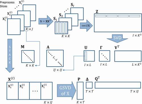
Zero Step – Preprocessing: Centering and scaling of the ${\mathbf{X}}_i^{\left(I\right)}$ slices are usual.

First Step – Interstructure: Cross-product matrices ${\mathbf{S}}_i={\mathbf{X}}_i^{\left(I\right)}{\left({\mathbf{X}}_i^{\left(I\right)}\right)}^{\mathrm{T}}$ are obtained and stored in a bigger matrix $\mathbf{Z}$, then its Singular Value Decomposition provides weights for the slices. In this step, every slice is represented onto the interstructure space denoted by:

$\mathbf{C}=\mathbf{Z}{\mathbf{Z}}^{\mathrm{T}}$

Second Step – Intrastructure: Slices are juxtaposed in a unique array ${\mathbf{X}}^{\left(I\right)}$. Matrix ${\mathbf{X}}^{\left(I\right)}$, masses matrix $\mathbf{M}$ and weights matrix $\mathbf{A}$, conform the triplet $\left({\mathbf{X}}^{\left(I\right)},\mathbf{A},\mathbf{M}\right)$. A generalized singular value decomposition (GSVD) is performed as follows:

${\mathbf{X}}^{\left(I\right)}=\mathbf{P}\mathbf{\Delta }{\mathbf{Q}}^{\mathrm{T}}$ with ${\mathbf{P}}^{\mathrm{T}}\mathbf{M}\mathbf{P}={\mathbf{Q}}^{\mathrm{T}}\mathbf{A}\mathbf{Q}=\mathbf{I}$

$x_{i\left(jk\right)}=\sum _{r=1}^R{p}_{ir}{\delta }_r{q}_{\left(jk\right)r},\left(jk\right)=\left(k-1\right)J+j$

In terms of statistical process control, the pioneering work done by Scepi (Scepi, 2002) was the first contribution of STATIS. However, a recent review on this multivariate method and its extensions is available in Abdi et al. (2012).

3.1.4. Parallel factors analysis (PARAFAC/CANDECOMP)

This method was developed in 1970 as PARAFAC (PARAllel FACtors) by Harshman and as CANDECOMP (CANOnical DECOMPosition) by Carrol and Chang, independent and simultaneously (Carroll & Chang, 1970; Harshman, 1970). Because of the nature of the decomposition, PARAFAC can be compared with a three-way PCA, with one scores and two loading sets of vectors stored in matrices. The PARAFAC method was successfully applied for statistical control and analysis in batch production (Meng et al., 2003).

In this case, Figure 8 reveals the decomposition of the three-way array $\left[\mathbf{X}\right]$, which can be described as follows:

$x_{ijk}=\sum _{r=1}^R\left(a_{ir}{b}_{jr}{c}_{kr}\right)$

Figure 8. PARAFAC decomposition

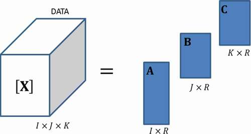
Where $a_{ir}$, $b_{jr}$ and $c_{kr}$ are elements of the matrices $\mathbf{A}$, $\mathbf{B}$ and $\mathbf{C}$ with $I\times R$, $J\times R$ and $K\times R$ orders, respectively.

The $K$-unfolded matrix ${\mathbf{X}}^{\left(K\right)}$ can be decomposed considering the Khatri-Rao product $\odot$ (Smilde et al., 2004) as:

${\mathbf{X}}^{\left(K\right)}=\mathbf{A}{\left(\mathbf{C}\odot \mathbf{B}\right)}^{\mathrm{T}},\hspace{0.17em}{\mathbf{A}}^{\mathrm{T}}\mathbf{A}={\mathbf{B}}^{\mathrm{T}}\mathbf{B}={\mathbf{C}}^{\mathrm{T}}\mathbf{C}=\mathbf{I}$

The computation of the sets is often slow and difficult to process; alternating least squares can be applied but is not much efficient. In addition, Kiers and Krijnen (1991) proposed a three steps method that improves the process and makes it more feasible to use.

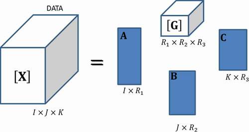
3.1.5. Tucker3

This method was first proposed by Tucker (1966) as shown in Figure 9. It can be used for higher dimensional data arrays; for instance, Tucker3 is a decomposition of $\left[\mathbf{X}\right]$ in four sets of loadings: $\mathbf{A}$, $\mathbf{B}$, $\mathbf{C}$ (as in PARAFAC), and $\left[\mathbf{G}\right]$ called ‘core’. Every observation can be expressed by:

$x_{ijk}=\sum _{r_1=1}^{R_1}\sum _{r_2=1}^{R_2}\sum _{r_3=1}^{R_3}\left(g_{r_1{r}_2{r}_3}{a}_{i{r}_1}{b}_{j{r}_2}{c}_{k{r}_3}\right)$

Figure 9. Tucker3 decomposition

where $a_{ir}$, $b_{jr}$ and $c_{kr}$ are elements of the three matrices $\mathbf{A}$, $\mathbf{B}$ and $\mathbf{C}$ with $I\times R_1$, $J\times R_2$ and $K\times R_3$ orders, respectively; and $g_{r_1{r}_2{r}_3}$ represent an element of the core $\left[\mathbf{G}\right]$ with order $R_1\times R_2\times R_3$.

The $K$-unfolded matrix ${\mathbf{X}}^{\left(K\right)}$ can be decomposed considering the $K$-unfolded core ${\mathbf{G}}^{\left(K\right)}$ and the Kronecker product $\otimes$ (Bellman, 1997) as:

${\mathbf{X}}^{\left(K\right)}=\mathbf{A}{\mathbf{G}}^{\left(K\right)}{\left(\mathbf{B}\otimes \mathbf{C}\right)}^{\mathrm{T}},\hspace{0.17em}{\mathbf{A}}^{\mathrm{T}}\mathbf{A}={\mathbf{B}}^{\mathrm{T}}\mathbf{B}={\mathbf{C}}^{\mathrm{T}}\mathbf{C}=\mathbf{I}$

Tucker3 model allows the contribution of much more factors than PCA and PARAFAC. Its core structure can describe the interaction level between these factors. When the core is a super identity matrix (diagonal full of ones, and zeros for the other elements), Tucker3 is equivalent to a PARAFAC analysis.

A comparison between MPCA, PARAFAC and Tucker3 was carried out in a semi-batch process in Louwerse & Smilde (2000).

3.1.6. Multiset canonical correlation analysis (MCCA)

MCCA extends the CCA constraint of ‘two sets of variables’ to the possibility of analyzing multiple sets at the same time. The purpose is to find weight vectors that maximize the correlation among the canonical variables. Within the multiway array $\left[\mathbf{X}\right]$, the $m^{th}$ weight vector ${\mathbf{U}}_k^m$ is obtained per $K$-slice from the SVD of a square matrix (Parra, 2018), and its corresponding canonical variable is computed as (Figure 10):

${\mathbf{Z}}_k^m={\mathbf{X}}_k{\mathbf{U}}_k^m,\hspace{0.17em}\frac{1}{I}\sum _{\mathit{i}=0}^{\mathit{n}}{\left({\mathbf{Z}}_k^m\right)}^{\mathrm{T}}\left({\mathbf{Z}}_k^m\right)=1$

Figure 10. MCCA method scheme

A more detailed math formulation and computing is available at (Jiang et al., 2018; Wang et al., 2017).

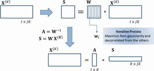
3.1.7. Multiway independent component analysis (MICA)

Often used to find independent signals that recreate some complex ones, MICA is a powerful method when MPCA does not fit the data in optimum ways. MICA is equivalent to apply ICA on an unfolded and mean-centered matrix ${\mathbf{X}}^{\left(K\right)}$ (as in MPCA), leading to the following result:

${\mathbf{X}}^{\left(K\right)}=\mathbf{A}\mathbf{S},\hspace{0.17em}\mathbf{A}=\left[{\mathbf{a}}_1\left|{\mathbf{a}}_2\right|\dots \left|{\mathbf{a}}_i\right|\dots |{\mathbf{a}}_I\right],$

where every ${\mathbf{a}}_i$ is statistically independent from each other

where $\mathbf{A}$ contains the scores, and $\mathbf{S}$, the information of the independent components from ${\mathbf{X}}^{\left(K\right)}$. These components, independent in a statistical context, are computed from weights matrix $\mathbf{W}=\left[{\mathbf{w}}_1\left|{\mathbf{w}}_2\right|\dots \left|{\mathbf{w}}_i\right|\dots |{\mathbf{w}}_I\right]\hspace{0.17em}$ such that $\mathbf{S}=\mathbf{W}{\mathbf{X}}^{\left(K\right)}$ so $\mathbf{A}={\mathbf{W}}^{-1}$.

The iterative procedure to estimate $\mathbf{W}$ consists of calculating weights vectors ${\mathbf{w}}_i$ with maximum non-gaussianity using an objective function and kurtosis as a non-gaussianity measurement. After every non-gaussianity maximization, ${\mathbf{w}}_k$ is decorrelated from the others previously computed. MICA decomposition is summarized in Figure 11.

Figure 11. MICA decomposition

This method is a big aid when non-Gaussian variables become difficult to manage. More details and math specifications are available at (Hyvärinen & Oja, 2000).

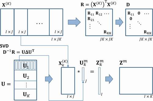
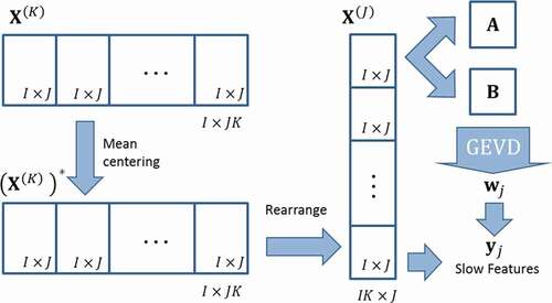
3.1.8. Multiway slow features analysis (MSFA)

MSFA is equivalent to apply SFA over a $J$-unfolded matrix $X^{\left(J\right)}$. The basic idea of SFA as described by Wiskott et al. (Wiskott, 1999; Wiskott & Sejnowski, 2002) is to find a series of instantaneous scalar input-output mapping functions so that the output signals vary as slow as possible. In this sense, the method’s goal is to find a set of constrained functions $y\left(t\right)$ called features with the capability to model a complex behavior from a dataset.

Optimization problem is described as follows: the functions $y\left(t\right)$ should have a ‘slow variation’, measured by the variance of its first-order derivative with respect of time; also present zero mean, unit variance, and decorrelation with each other.

The MSFA process starts with $K$-unfolding of $\left[\mathbf{X}\right]$ to perform mean centering of $X^{\left(K\right)}$ for obtaining ${\left({\mathbf{X}}^{\left(K\right)}\right)}^{\ast }$; then, preprocessed ${\left({\mathbf{X}}_k^{\left(K\right)}\right)}^{\ast }$ slices are rearranged to conform a $J$-unfolded matrix ${\mathbf{X}}^{\left(J\right)}$.

Considering the observation vector ${\mathbf{x}}_i^{\left(J\right)}$ as the $i^{th}$ row of ${\mathbf{X}}^{\left(J\right)}$, covariance matrices ${\mathbf{A}}_{J\times J}$and ${\mathbf{B}}_{J\times J}$ are defined as follows:

$\mathbf{A}=\frac{1}{IK-2}\sum _{i=2}^{IK}\left({\mathbf{x}}_i-{\mathbf{x}}_{i-1}\right){\left({\mathbf{x}}_i-{\mathbf{x}}_{i-1}\right)}^{\mathrm{T}}$

$\mathbf{B}=\frac{1}{IK-1}\sum _{i=1}^{IK}\left({\mathbf{x}}_i\right){\left({\mathbf{x}}_i\right)}^{\mathrm{T}}$

Solving the optimization problem of SFA leads to the generalized eigenvalue problem (GEVD):

$\mathbf{A}{\mathbf{w}}_j={\lambda }_j\mathbf{B}{\mathbf{w}}_j$

Finally, each $j$ slow feature for every observation ${\mathbf{x}}_i^{\left(J\right)}$ computed as $y_j={\mathbf{w}}_j^{\mathrm{T}}{\mathbf{x}}_i^{\left(J\right)}$ . This allows to project new observations using ${\mathbf{w}}_j$ vectors as depicted in Figure 12.

Figure 12. MSFA method scheme

For a more detailed and extensive analysis of the method, see Zhang et al. (2017).

3.2. Non-dimensionality reduction

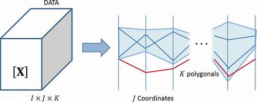
3.2.1. Parallel coordinates

Parallel coordinates as a graphical representation system were proposed by Alfred Inselberg from which multivariate data could be represented in a two-dimensional system (Inselberg & Dimsdale, 1990).

Each $K$ observation of $\left[\mathbf{X}\right]$ within $I$-slices is represented in $J$variables by a polygonal of $J-1$ sides. In addition, the correlation analysis between $J$ variables focuses on intersections from polygonals that are constructed from raw $I$-slices (Inselberg, 2009; Wegman, 1990). When lines present a similar behavior, this tool is very useful in identifying clusters between observations (Inselberg, 2009).

In this sense, parallel coordinates can be used for ‘visual clustering’, i.e. to find groups of similar points based on visual features such as the proximity of lines or line density (Heinrich & Weiskopf, 2013). For control and monitoring, parallel coordinates capacity for clustering and summarization have great importance in plotting confidence regions (Dunia et al., 2012) as illustrated in Figure 13.

Figure 13. Parallel coordinates confidence region

4. Applications timeline

In 1994, Nomikos and MacGregor simulated data from an industrial process for semi-batch emulsion polymerization of styrene-butadiene to make a latex rubber (SBR) was considered to validate the monitoring of batches using MPCA on historical data (Nomikos & MacGregor, 1994). This kind of approach has many advantages because allows to control the quality of the process and its products even if there’s not a deep understanding of the process dynamics. Kosanovich et al. (1994) applied MPCA on real data of an industrial single batch reactor, including stages separation. This improved the detection of the principal causes of batch failure, like variable reactor temperature (stage 1) and heat input rate (stage 2).

In 1995, Nomikos and MacGregor used MPCA to summarize variables and time of real data from industrial batch polymerization reactor into low-dimensional spaces, which allowed to monitor the process visually (Nomikos & MacGregor, 1995b). Also, Kourti et al. (1995) applied MPLS technique to real data of the same industrial batch polymerization process with one and two stages, considering multiblock arrangements. They constructed monitoring charts which helped to detect faults quickly and easily, allowing the isolation of the possible causes of the fault. In addition, Nomikos and MacGregor (1995a) pointed out that MPLS can be easily implemented for almost any batch or semi-batch process. They applied this technique on simulated data of a polymerization process to control not only process variable trajectories but also final quality measurements when the batch production ends.

Gallagher et al. (1996) showed that using MPCA on real data for a nuclear waste storage tank monitoring helped to monitor the process and identify differences between the start-up period and the calibration period. The main advantage of this method is shown in terms of input data reduction.

MPCA was also applied in 1996 with simulated data of a batch polymerization reactor study, based on ‘pilot-scale methyl methacrylate’ (MMA) reactor, the proposed method used special confidence bounds and validated the capacity of the method to monitor the data (Martin et al., 1996). Control strategies using MPCA also help to improve process understanding, as shown in Kosanovich et al. (1996), where the major sources of variability were identified within the polymerization process. Extensions of MPCA like the use on Nonlinear PCA were considered in Dong and McAvoy (1996) to improve the performance of the monitoring scheme in two sets of simulated data: one for emulsion polymerization and the other of a two-stage jacketed exothermic batch chemical reactor.

Process knowledge was combined in 1998 with an MPCA and MPLS approach as found in Neogi and Schlags (1998). The combination was applied to real data of emulsion polymer production to detect potential anomalous batches, exact time of abnormalities and possible causes or variability. For instance, in 1999 a successful MPCA application was developed based on real historical data from industrial batch production of PVC via polymerization process (Tates et al., 1999). Also, Martin et al. (1999) proposed the application of MPCA on simulated data for a pilot-scale MMA reactor process, combined with inverse MPLS (IMPLS) led to predict desired profiles for variables which enhanced the control and monitoring performance.

MPCA was considered by Chen and Liu (2000) for its use, at 2000, in two batch processes: a catalyst reaction (simulation) and a wafer plasma etching (real). This strategy resulted simple and easy, but still capable of dimensionality reduction of the dataset to few factors in a latent space. A comparison between MPCA, PARAFAC, and TUCKER3 was done in Louwerse and Smilde (2000) using simulated data of a semi-batch emulsion polymerization of SBR. The main conclusion of this work declares that there is no ‘king method’, each of them has its advantages and disadvantages, it will depend on the data and analysis goals. For 2001, the same simulated dataset was used by Yuan and Wang (2001) to test a combination of MPCA and wavelet analysis to deal with the dynamic evolution of variables. PARAFAC2 was also considered in Wise et al. (2001) for fault detection and diagnosis in a semiconductor etch process; the method was compared with MPCA, PARAFAC, and PCA. The main advantage reported of PARAFAC2 was the ability to deal with data records of variable length without preprocessing requirements.

In 2003, the benchmark process of fed-batch penicillin production (simulated data) was considered by Ündey et al. (2003) for an MPLS application combining Iterative Learning Control (ILC) and Manipulated Variable Trajectories (MVTs). This strategy helped to predict the end-of-batch quality measurements and increase the process control performance. In Meng et al. (2003), a simulated process of semi-batch emulsion polymerization was employed to highlight the capacity of methods like MPCA and PARAFAC to monitor batch processes. The author assessed that there will always be a delay in the signaling at the start (unless it is a major fault); however, more sophisticated methods will not be required.

In 2004, researchers showed that MPCA could provide a powerful tool for estimating trajectories for variables and its expected behavior. They applied this method on a real Nylon polymerization process data and a simulated dataset of batches for an emulsion polymerization process (García-Muñoz et al., 2004). Same year, Lee et al. (2004) added a Kernel analysis to conventional MPCA to perform MKPCA on a fed-batch penicillin production simulated dataset. This approach was able to identify significant deviations that could cause a lower quality of the final products. Also, it could manage nonlinear relationships in the process variables leading to a better performance, if compared to MPCA. A different approach was considered by Albazzaz (2004) and Yoo et al. (2004) when they applied MICA to control two simulated processes: a semi-batch polymerization reactor and fed-batch penicillin production, respectively. Results from these analyses exhibited a superior performance on monitoring if compared to MPCA, this was achieved because MICA can extract more interpretable results in the main components when non-gaussianity is presented in the data.

In 2005, Gourvénec et al. (2005) exploited the STATIS method to analyze three-way arrays in two sets of real data for control and monitoring pharmaceutical batch process of maleic acid formation and yeast bakery production. This approach offers visualization tools of high quality and is a big aid for dealing with batches of variable duration, preserving the structure of the dimensions (times, variables, batches). In addition, MPCA was used as a reliable diagnostic tool in 2006, as shown in Cho et al. (2006), where it was applied to a real PVC batch process and a simulated dataset of fed-batch penicillin process. By 2007, MPCA and MPLS were used in Ferreira et al. (2007) for a real dataset of industrial pilot-scale fermentation where process knowledge was improved, and abnormal variations were detected.

Advances in control monitoring appeared in 2008 with an MPCA variant called Dynamic PCA, proposed by Doan and Srinivasan (2008) to monitor a simulated fermentation process. The main results from this research were process phases recognition and fault sensitivity improvement. On the other hand, Lin and Chen (2008) tested MPLS performance combined with ILC and MVTs, similar to the work presented in Ündey et al. (2003). In this application, of simulated data, the control objective was to maintain the concentrations of two reaction products at predefined desired levels after the batch run finishes. The goal was reached, tracking quality in the batch operation process using only the information contained in the historical database rather than detailed knowledge of the operation process model.

STATIS approach was considered by Niang et al. (2009) for control monitoring which allowed to project trajectories of variables within the batch and to detect significant differences when compared to expected trajectories from historical data. Data used in this study corresponded to a batch polymerization reactor (real) and an industrial process with batches of variable duration (simulated). STATIS was also applied by Fogliatto and Niang (2009) using simulated data for a process with batches of variable duration. Off-line and on-line control were achieved, time-wise monitoring was performed, and fault times were correctly identified.

Fed-batch penicillin fermentation, a simulated process, was studied once more in 2013 by Yu et al. (2013) to validate the monitor ability of MICA in batch processes. The proposal has a superior capability for multiphase fault detection and diagnosis, and, not only the abnormal events can be precisely captured but also the major faulty variables were accurately identified. STATIS was used in Niang et al. (2013) to control a batch polymerization reactor process (simulated). The results illustrate the good performance of the method for off-line and on-line monitoring. Another STATIS application was developed in 2015, as detailed in Filho and Luna (2015) where a toy model (simulation) of an industrial process was considered to test the control abilities of the method. The monitoring scheme and the non-parametric control analyses demonstrated its discriminative ability by means of correlation structure preservation between variables and time. Slow Features Analysis (SFA) and Canonical Correlation Analysis (CCA) were applied to the batch scheme in 2017 using, in both cases, simulation studies of a numerical example and the well-known fed-batch penicillin fermentation process. First, Zhang et al. (2017) applied the multiway-kernel version of SFA (MKSFA) and others of similar use like MKPCA, MKICA, and BDKPCA, however, they enhanced the monitoring capacity considering a global preserving scope, leading to MGKSFA. This approach was able to manage nonlinear characteristics of the variables and inherent time-varying dynamics of the data. The proposed method (MGKSFA) performed better than the others in the comparison in terms of fault detection time and rate. After this, Wang et al. (2017) applied multiset CCA (MCCA) for parallel-running processes which allowed to monitor individual and joint features. The case studies validated the efficiency of the method, in terms of control and monitoring, of the parallel processes.

Finally, for 2018, a new MPCA exploitation showed up in Cho and Kim (2018) with real data from an industrial PVC batch process. The method took full advantage of the information contained in data, to detect abnormalities of new batches earlier. An extension of the previous MCCA application can be found in Jiang et al. (2018) where a numerical example and a real data application on injection molding machine were used as case studies to test the approach, improved with consideration of key operation units. The proposed monitoring scheme detected a local fault incorporating both the variables within the key units and the information from other related units. Another application of STATIS, in its Dual version and combined with Parallel Coordinates (PARCOORDS) was proposed in Ramos-Barberán et al. (2018) where a numerical example and the well-known benchmark process of fed-batch penicillin production were considered for validation. Monitoring was achieved without special considerations for data distribution, bagplots based regions enhanced the discrimination capacity to detect faults, and visualization of reference/new batches using PARCOORDS became a powerful tool for abnormal pattern recognition.

Reviewed methods and its applications to control batch processes are summarized in Table 3, where most of these are related to chemical industrial processes.

Table 3. MSPC applications for batch process control

Nº	TITLE	AUTHOR	YEAR	METHOD
1	Monitoring batch processes using multiway principal component analysis	Nomikos, MacGregor	1994	MPCA
2	Multi-way PCA applied to an industrial batch process	Kosanovich, Piovoso, Dahl, MacGregor, Nomikos	1994	MPCA
3	Multivariate SPC Charts for Monitoring Batch Processes	Nomikos, MacGregor	1995	MPCA
4	Analysis, monitoring and fault diagnosis of batch processes using multiblock and multiway PLS	Kourti, Nomikos, MacGregor	1995	MPLS (+Multiblock)
5	Multi-way partial least squares in monitoring batch processes	Nomikos, MacGregor	1995	MPLS
6	Application of multi-way principal components analysis to nuclear waste storage tank monitoring	Gallagher, Wise, Stewart	1996	MPCA
7	Batch process monitoring for consistent production	Martin, Morris, Papazoglou, Kiparissides	1996	MPCA
8	Improved Process Understanding Using Multiway Principal Component Analysis	Kosanovich, Dahl, Piovoso	1996	MPCA
9	Batch tracking via nonlinear principal component analysis	Dong, McAvoy	1996	MPCA (+NLPCA +Multistage)
10	Multivariate Statistical Analysis of an Emulsion Batch Process	Neogi, Schlags	1998	MPCA, MPLS
11	Monitoring a PVC Batch Process with Multivariate Statistical Process Control Charts	Tates, Louwerse, Smilde, Koot, Berndt	1999	MPCA
12	Manufacturing performance enhancement through multivariate statistical process control	Martin, Morris, Kiparissides	1999	MPCA, MPLS (IMPLS)
13	Post analysis on different operating time processes using orthonormal function approximation and multiway principal component analysis	Chen, Liu	2000	MPCA
14	Multivariate statistical process control of batch processes based on three-way models	Louwerse, Smilde	2000	MPCA, PARAFAC, TUCKER3
15	Multilevel PCA and Inductive learning for knowledge extraction from operational data of batch processes	Yuan, Wang	2001	MPCA
16	Application of PARAFAC2 to fault detection and diagnosis in semiconductor etch	Wise	2001	PARAFAC, MPCA, MPLS
17	Online Batch/Fed-Batch Process Performance Monitoring, Quality Prediction, and Variable-Contribution Analysis for Diagnosis	Ündey, Ertunç, Çinar	2003	MPLS (+ILC, MVTs)
18	On-line monitoring of batch processes using a PARAFAC representation	Meng	2003	PARAFAC + MPCA
19	Model Predictive Monitoring for Batch Processes	García-Muñoz, Kourti, MacGregor	2004	MPCA
20	Fault detection of batch processes using multiway kernel principal component analysis	Jong-Min Lee, Yoo, In-Beum Lee	2004	MPCA (+Multiway Kernel PCA)
21	Statistical Process Control Charts for Batch Operations Based on Independent Component Analysis	Albazzaz, Wang	2004	MICA
22	On-line monitoring of batch processes using multiway independent component analysis	Yoo, Jong-Min Lee, Vanrolleghem, In-Beum Lee	2004	MICA
23	Monitoring batch processes with the STATIS approach	Gourvénec, Stanimirova, Saby, Airiau, Massart	2005	STATIS
24	Online monitoring and diagnosis of batch processes: empirical model-based framework and a case study	Cho, Kim, Jeong	2006	MPCA
25	Study of the application of multiway multivariate techniques to model data from an industrial fermentation process	Ferreira, Lopes, Menezes	2007	MPCA, MPLS
26	Online monitoring of multi-phase batch processes using phase-based multivariate statistical process control	Doan, Srinivasan	2008	MPCA (+Dynamic PCA)
27	Two-Step MPLS-Based Iterative Learning Control for Batch Processes	Chen, Lin	2008	MPLS
28	Batch Process Monitoring by Three-way Data Analysis Approach	Niang, Fogliatto, Saporta	2009	STATIS
29	Multivariate Statistical Control of Batch Processes with Variable Duration	Fogliatto, Niang	2009	STATIS
30	Multiway Independent Component Analysis Mixture Model and Mutual Information Based Fault Detection and Diagnosis Approach of Multiphase Batch Processes	Yu, Chen, Rashid	2013	MICA
31	Non parametric on-line control of batch processes based on STATIS and clustering	Niang, Fogliatto, Saporta	2013	STATIS
32	Multivariate quality control of batch processes using STATIS	Filho, Luna	2015	STATIS
33	Batch Process Monitoring Based on Multiway Global Preserving Kernel Slow Feature Analysis	Zhang, Tian, Deng	2017	MSFA (+Global preserving Kernel SFA, BDKPCA, MKICA, MKPCA)
34	Joint-Individual Monitoring of Parallel-Running Batch Processes Based on MCCA	Wang, Jiang, Li, Lizhi	2017	MCCA
35	A Method for Predicting Future Observations in the Monitoring of a Batch Process	Cho, Kim	2003	MPCA
36	Multivariate Statistical Monitoring of Key Operation Units of Batch Processes Based on Time-Slice CCA	Jiang, Gao, Yi, Yan	2018	MCCA
37	Batch process control and monitoring: a Dual STATIS and Parallel Coordinates (DS-PC) approach	Ramos-Barberán, Hinojosa-Ramos, Ascencio-Moreno, Vera, Ruiz-Barzola, Galindo-Villardón	2018	STATIS, PARCOORDS (+Dual STATIS)

5. Results and discussion

MSPC applied to batches usually performs dimensionality reduction over the multilinear array analyzed. Dataset unfolding is the main step towards consideration of this multiway analysis as a two-way problem, involving matrices instead of arrays. Depending on the chosen method and the research objective, results obtained are biased by slicing consideration and unfolding direction.

In addition, dimensionality reduction methods rely on SVD to solve their corresponding optimization problems considering restrictions and cost functions (Rosipal & Krämer, 2005). Therefore, a comparison between these methods can be done.

The preferred method, for its ease of interpretation and well-known implementation, is MPCA, nevertheless, more robust approaches can be slightly better in terms of fault detection rates (Zhang et al., 2017). While MPCA maximizes the explained variance along one array, MCCA focuses on data correlations’ maximization between selected slices, and MPLS computes maximum covariance between two arrays (Rosipal & Krämer, 2005).

Tucker3 and PARAFAC models need less parameters than MPCA to decompose the multilinear array. However, MPCA captures more variance than these models. On the other hand, Tucker3 and PARAFAC principal components can be computed for every dimension in the batch (Louwerse & Smilde, 2000).

When non-gaussianity is presented in the dataset, MICA exhibits an advantage over MPCA due to a better extraction of latent variables and data optimum fit. This characteristic allows to discriminate any unusual behavior within batches. Both MSFA and MICA are usually applied in blind source separation (Zafeiriou et al., 2013); analogous to batches variables, they perform latent variables extraction, with a crucial difference for MSFA where the variation of extracted features is smoothed.

Parallel coordinates, as a non-dimensionality reduction method, differ from the others because no latent variables are needed, preserving the multilinear nature of the dataset. Values of each variable and observation within batches can be displayed in an all-in-one system, which allows to identify local patterns and their global dynamics behavior.

6. Conclusions

To sum up, the present review does not pretend to select the best method; instead, it shows that each one of the described techniques may perform better under specific conditions, considering batch process practical implications and researchers optimization goals. Finally, the combination of analyzed methods widens their application under different scenarios, helps to overcome their limitations, and enhances their individual advantages in terms of results interpretation.

Disclosure statement

No potential conflict of interest was reported by the authors.

References

- Abdi, H. (2010). Partial least squares regression and projection on latent structure regression (PLS Regression). Wiley interdisciplinary reviews. Computational statistics, 2(1), 97–106. https://doi.org/https://doi.org/10.1002/wics.51
- Abdi, H., & Williams, L. J. (2010). Principal component analysis. Wiley interdisciplinary reviews. Computational statistics, 2(4), 433–459. https://doi.org/https://doi.org/10.1002/wics.101
- Abdi, H., Williams, L. J., Valentin, D., & Bennani-Dosse, M. (2012). STATIS and DISTATIS: Optimum multitable principal component analysis and three way metric multidimensional scaling. Wiley interdisciplinary reviews. Computational statistics, 4(2), 124–167. https://doi.org/https://doi.org/10.1002/wics.198
- Albazzaz, H. (2004). Statistical process control charts for batch operations based on independent component analysis. Industrial & Engineering Chemistry Research, 43(21), 6731–6741. https://doi.org/https://doi.org/10.1021/ie049582+
- Bellman, R. (1997). Introduction to matrix analysis (2nd ed. ; ed., R. E. O’Malley.). Classics in Applied Mathematics.
- Bersimis, S., Psarakis, S., & Panaretos, J. (2007). Multivariate statistical process control charts: An overview. Quality and Reliability Engineering International, 23(5), 517–543. https://doi.org/https://doi.org/10.1002/qre.829
- Carroll, J. D., & Chang, -J.-J. (1970). Analysis of individual differences in multidimensional scaling via an n-way generalization of “Eckart-Young” decomposition. Psychometrika, 35(3), 283–319. https://doi.org/https://doi.org/10.1007/BF02310791
- Chen, J., & Liu, J. (2000). Post analysis on different operating time processes using orthonormal function approximation and multiway principal component analysis. Journal of process control, 10(5), 411–418. https://doi.org/https://doi.org/10.1016/S0959-1524(00)00016-0
- Cho, H. W., & Kim, K. J. (2018). A method for predicting future observations in the monitoring of a batch process. Journal of Quality Technology, 35(1), 59–69. https://doi.org/https://doi.org/10.1080/00224065.2003.11980191
- Cho, H. W., Kim, K. J., & Jeong, M. K. (2006). Online monitoring and diagnosis of batch processes: Empirical model-based framework and a case study. International Journal of Production Research, 44(12), 2361–2378. https://doi.org/https://doi.org/10.1080/00207540500422130
- Doan, X. T., & Srinivasan, R. (2008). Online monitoring of multi-phase batch processes using phase-based multivariate statistical process control. Computers & chemical engineering, 32(1–2), 230–243. https://doi.org/https://doi.org/10.1016/j.compchemeng.2007.05.010
- Dong, D., & McAvoy, T. J. (1996). Batch tracking via nonlinear principal component analysis. AIChE Journal, 42(8), 2199–2208. https://doi.org/https://doi.org/10.1002/aic.690420810
- Dunia, R., Edgar, T., & Nixon, M. (2012). Process monitoring using principal components in parallel coordinates. American Institute of Chemical Engineers Journal, 59(2), 1–12. https://doi.org/https://doi.org/10.1002/aic.13846
- Escoufier, Y. (1987). Three-mode data analysis: The STATIS method. In B. Fichet & C. Lauro (Eds.), Methods for multidimensional data analysis (pp. 259–272). ECAS.
- Ferreira, A. P., Lopes, J. A., & Menezes, J. C. (2007). Study of the application of multiway multivariate techniques to model data from an industrial fermentation process. Analytica chimica acta, 595(1–2), 120–127. https://doi.org/https://doi.org/10.1016/j.aca.2007.05.007
- Filho, D. M., & Luna, L. P. (2015). Multivariate quality control of batch processes using STATIS. International journal of advanced manufacturing technology, 82(5–8), 867–875. https://doi.org/https://doi.org/10.1007/s00170-015-7428-0
- Flores-Cerrillo, J., & MacGregor, J. F. (2005). Iterative learning control for final batch product quality using partial least squares models. Industrial & engineering chemistry research, 44(24), 9146–9155. https://doi.org/https://doi.org/10.1021/ie048811p
- Fogliatto, F. S., & Niang, N. (2009). Multivariate statistical control of batch processes with variable duration. IEEE International Conference on Industrial Engineering and Engineering Management, 434–438. Hong Kong, China. https://doi.org/https://doi.org/10.1109/IEEM.2009.5373316
- Gallagher, N. B., Wise, B. M., & Stewart, C. W. (1996). Application of multi-way principal components analysis to nuclear waste storage tank monitoring. Computers & chemical engineering, 20(96), S739–S744. https://doi.org/https://doi.org/10.1016/0098-1354(96)00131-7
- García-Muñoz, S., Kourti, T., & MacGregor, J. F. (2004). Model predictive monitoring for batch processes. Industrial & engineering chemistry research, 43(18), 5929–5941. https://doi.org/https://doi.org/10.1021/ie034020w
- Geladi, P., Manley, M., & Lestander, T. (2003). Scatter plotting in multivariate data analysis. Journal of chemometrics, 17(8–9), 503–511. https://doi.org/https://doi.org/10.1002/cem.814
- Gourvénec, S., Stanimirova, I., Saby, C. A., Airiau, C. Y., & Massart, D. L. (2005). Monitoring batch processes with the STATIS approach. Journal of chemometrics, 19(5–7), 288–300. https://doi.org/https://doi.org/10.1002/cem.931
- Harshman, R. A. (1970). Foundations of the PARAFAC procedure: Models and conditions for an “explanatory” multimodal factor analysis. UCLA Working Papers in Phonetics, 16(10), 1–84. https://www.psychology.uwo.ca/faculty/harshman/wpppfac0.pdf
- Heinrich, J., & Weiskopf, D. (2013). State of the art of parallel coordinates. Eurographics Conference on Visualization (EuroVis), 95–116. Leipzig, Germany. https://doi.org/https://doi.org/10.2312/conf/EG2013/stars/095-116
- Hotelling, H. (1947). Multivariate quality control illustrated by air testing of sample bombsights. In C. Eisenhart, M. W. Hastay, & W. A. Wallis (Eds.), Techniques of statistical analysis (pp. 111–184). McGraw Hill.
- Hyvärinen, A., & Oja, E. (2000). Independent component analysis: Algorithms and applications. Neural Networks, 13(4–5), 411–430. https://doi.org/https://doi.org/10.1016/S0893-6080(00)00026-5
- Inselberg, A. (2009). Parallel coordinates: Intelligent multidimensional visualization (D. Plemenos & G. Miaoulis, eds.)). Springer.
- Inselberg, A., & Dimsdale, B. (1990). Parallel coordinates: A tool for visualizing multi-dimensional geometry. Proceedings of the First IEEE Conference on Visualization, San Francisco, CA, USA. 361–378. http://dl.acm.org/citation.cfm?id=949531.949588
- Jiang, Q., Gao, F., Yi, H., & Yan, X. (2018). Multivariate statistical monitoring of key operation units of batch processes based on time-slice CCA. IEEE Transactions on Control Systems Technology, 27(3), 1368–1375. https://doi.org/https://doi.org/10.1109/TCST.2018.2803071
- Kiers, H. A. L., & Krijnen, W. P. (1991). An efficient algorithm for PARAFAC of three-way data with large numbers of observation units. Psychometrika, 56(1), 147–152. https://doi.org/https://doi.org/10.1007/BF02294592
- Kosanovich, K. A., Dahl, K. S., & Piovoso, M. J. (1996). Improved process understanding using multiway principal component analysis. Industrial & engineering chemistry research, 35(1), 138–146. https://doi.org/https://doi.org/10.1021/ie9502594
- Kosanovich, K. A., Piovoso, M. J., Dahl, K. S., MacGregor, J. F., & Nomikos, P. (1994). Multi-way PCA applied to an industrial batch process. American Control Conference, Baltimore, MD, USA. 1294–1298. https://doi.org/https://doi.org/10.1109/acc.1994.752268
- Kourti, T., Nomikos, P., & MacGregor, J. F. (1995). Analysis, monitoring and fault diagnosis of batch processes using multiblock and multiway PLS. Journal of process control, 5(4), 277–284. https://doi.org/https://doi.org/10.1016/0959-1524(95)00019-M
- L’Hermier Des Plantes, H. (1976). Structuration des Tableaux à Trois Indices de la Statistique: Théorie et Application d’une Méthode d’ Analyse Conjointe. Université des Sciences et Techniques du Languedoc.
- Lavit, C., Escoufier, Y., Sabatier, R., & Traissac, P. (1994). The ACT (STATIS method). Computational statistics & data analysis, 18(1), 97–119. https://doi.org/https://doi.org/10.1016/0167-9473(94)90134-1
- Lee, J. M., Yoo, C. K., & Lee, I. B. (2004). Fault detection of batch processes using multiway kernel principal component analysis. Computers & chemical engineering, 28(9), 1837–1847. https://doi.org/https://doi.org/10.1016/j.compchemeng.2004.02.036
- Lewis, D. (2014). Control charts for batch processes. In Wiley StatsRef: Statistics reference online (pp. 1–9). John Wiley & Sons.
- Lin, K., & Chen, J. (2008). Two-step MPLS-based iterative learning control for batch processes. International MultiConference of Engineers and Computer Scientists, 2169(1), 1298–1303. https://pdfs.semanticscholar.org/7b59/3d8949b1cafb1b97a945d50ae6eb839306c0.pdf
- Louwerse, D. J., & Smilde, A. K. (2000). Multivariate statistical process control of batch processes based on three-way models. Chemical engineering science, 55(7), 1225–1235. https://doi.org/https://doi.org/10.1016/S0009-2509(99)00408-X
- Lu, H., Plataniotis, K. N., & Venetsanopoulos, A. N. (2008). MPCA: Multilinear principal component analysis of tensor objects. IEEE Transactions on Neural Networks, 19(1), 18–39. https://doi.org/https://doi.org/10.1109/TNN.2007.901277
- Macgregor, J. F. (1997). Using on-line process data to improve quality: Challenges for statisticians. International Statistical Review, 65(3), 309–323. https://doi.org/https://doi.org/10.1111/j.1751-5823.1997.tb00311.x
- Martin, E. B., Morris, A. J., & Kiparissides, C. (1999). Manufacturing performance enhancement through multivariate statistical process control. Annual reviews in control, 23(1), 35–44. https://doi.org/https://doi.org/10.1016/S1367-5788(99)00005-X
- Martin, E. B., Morris, A. J., Papazoglou, M. C., & Kiparissides, C. (1996). Batch process monitoring for consistent production. Computers & chemical engineering, 20(96), S599–S604. https://doi.org/https://doi.org/10.1016/0098-1354(96)00109-3
- Meng, X., Morris, A. J., & Martin, E. B. (2003). On-line monitoring of batch processes using a PARAFAC representation. Journal of chemometrics, 17(1), 65–81. https://doi.org/https://doi.org/10.1002/cem.776
- Neogi, D., & Schlags, C. E. (1998). Multivariate statistical analysis of an emulsion batch process. Industrial & engineering chemistry research, 37(10), 3971–3979. https://doi.org/https://doi.org/10.1021/ie980243o
- Niang, N., Fogliatto, F. S., & Saporta, G. (2009). Batch process monitoring by three-way data analysis approach. Applied Stochastic Models and Data Analysis, 294–298. https://www.researchgate.net/publication/228424412_Batch_Process_Monitoring_by_Three-way_Data_Analysis_Approach
- Niang, N., Fogliatto, F. S., & Saporta, G. (2013). Non parametric on-line control of batch processes based on STATIS and clustering. Journal de La Société Francaise de Statistique, 154(3), 124–142. https://cedric.cnam.fr/fichiers/art_2896.pdf
- Nomikos, P., & MacGregor, J. F. (1994). Monitoring batch processes using multiway principal component analysis. AIChE Journal, 40(8), 1361–1375. https://doi.org/https://doi.org/10.1002/aic.690400809
- Nomikos, P., & MacGregor, J. F. (1995a). Multi-way partial least squares in monitoring batch processes. Chemometrics and Intelligent Laboratory Systems, 30(1), 97–108. https://doi.org/https://doi.org/10.1016/0169-7439(95)00043-7
- Nomikos, P., & MacGregor, J. F. (1995b). Multivariate SPC charts for monitoring batch processes. Technometrics, 37(1) 41–59. https://doi.org/https://doi.org/10.1080/00401706.1995.10485888
- Parra, L. C. (2018). Multi-set canonical correlation analysis simply explained. Nips. http://arxiv.org/abs/1802.03759
- Ramos-Barberán, M., Hinojosa-Ramos, M. V., Ascencio-Moreno, J., Vera, F., Ruiz-Barzola, O., & Galindo-Villardón, M. P. (2018). Batch process control and monitoring: A dual STATIS and parallel coordinates (DS-PC) approach. Production and Manufacturing Research, 6(1), 470–493. https://doi.org/https://doi.org/10.1080/21693277.2018.1547228
- Rosipal, R., & Krämer, N. (2005). Overview and Recent Advances in Partial Least Squares. In: Saunders C., Grobelnik M., Gunn S., Shawe-Taylor J. (eds). Subspace, Latent Structure and Feature Selection. SLSFS 2005. Lecture Notes in Computer Science, vol 3940, (pp. 34–51). Springer, Berlin, Heidelberg. https://doi.org/https://doi.org/10.1007/11752790_2
- Scepi, G. (2002). Parametric and non parametric multivariate quality control charts. In C. Lauro, J. Antoch, V. E. Vinzi, & G. Saporta (Eds.), Multivariate total quality control: Foundation and recent advances (pp. 163–189). Physica-Verlag HD.
- Smilde, A., Bro, R., & Geladi, P. (2004). Multi-way analysis. Applications in the chemical sciences (L. John Wiley & Sons ed.). https://doi.org/https://doi.org/10.1002/0470012110
- Tates, A. A., Louwerse, D. J., Smilde, A. K., Koot, G. L. M., & Berndt, H. (1999). Monitoring a PVC batch process with multivariate statistical process control charts. Industrial & engineering chemistry research, 38(12), 4769–4776. https://doi.org/https://doi.org/10.1021/ie9901067
- Tucker, L. R. (1966). Some mathematical notes on three-mode factor analysis. Psychometrika, 31(3), 279–311. https://doi.org/https://doi.org/10.1007/BF02289464
- Ündey, C., Ertunç, S., & Çinar, A. (2003). Online batch/fed-batch process performance monitoring, quality prediction, and variable-contribution analysis for diagnosis. Industrial & engineering chemistry research, 42(20), 4645–4658. https://doi.org/https://doi.org/10.1021/ie0208218
- Wang, Y., Jiang, Q., Li, B., & Cui, L. (2017). Joint-individual monitoring of parallel-running batch processes based on MCCA. IEEE Access, 6, 13005–13014. https://doi.org/https://doi.org/10.1109/ACCESS.2017.2784097
- Wegman, E. (1990). Hyperdimensional data analysis using parallel coordinates. Journal of the American Statistical Association, 85(411), 664–675. https://doi.org/https://doi.org/10.1080/01621459.1990.10474926
- Wise, B. M., Gallagher, N. B., & Martin, E. B. (2001). Application of PARAFAC2 to fault detection and diagnosis in semiconductor etch. Journal of chemometrics, 15(4), 285–298. https://doi.org/https://doi.org/10.1002/cem.689
- Wiskott, L. (1999). Learning invariance manifolds. Neurocomputing, 26–27, 925–932. https://doi.org/https://doi.org/10.1016/S0925-2312(99)00011-9
- Wiskott, L., & Sejnowski, T. J. (2002). Slow feature analysis: Unsupervised learning of invariances. Neural computation, 14(4), 715–770. https://doi.org/https://doi.org/10.1162/089976602317318938
- Wold, S., Geladi, P., Esbensen, K., & Öhman, J. (1987). Multi-way principal components and PLS-Analysis. Journal of chemometrics, 1(1), 41–56. https://doi.org/https://doi.org/10.1002/cem.1180010107
- Woodall, W. H., & Montgomery, D. C. (1999). Research issues and ideas in statistical process control. Journal of Quality Technology, 31(4), 376–386. https://doi.org/https://doi.org/10.1080/00224065.1999.11979944
- Yoo, C. K., Lee, J. M., Vanrolleghem, P. A., & Lee, I. B. (2004). On-line monitoring of batch processes using multiway independent component analysis. Chemometrics and Intelligent Laboratory Systems, 71(2), 151–163. https://doi.org/https://doi.org/10.1016/j.chemolab.2004.02.002
- Yu, J., Chen, J., & Rashid, M. M. (2013). Multiway independent component analysis mixture model and mutual information based fault detection and diagnosis approach of multiphase batch processes. AIChE Journal, 59(8), 2761–2779. https://doi.org/https://doi.org/10.1002/aic.14051
- Yuan, B., & Wang, X. Z. (2001). Multilevel PCA and inductive learning for knowledge extraction from operational data of batch processes. Chemical engineering communications, 185(October2014), 201–221. https://doi.org/https://doi.org/10.1080/00986440108912863
- Zafeiriou, L., Nicolaou, M. A., Zafeiriou, S., Nikitidis, S., & Pantic, M. (2013). Learning slow features for behaviour analysis. Proceedings of the IEEE International Conference on Computer Vision, Sydney, Australia. 2840–2847. https://doi.org/https://doi.org/10.1109/ICCV.2013.353
- Zhang, H., Tian, X., & Deng, X. (2017). Batch process monitoring based on multiway global preserving kernel slow feature analysis. IEEE Access, 5, 2696–2710. https://doi.org/https://doi.org/10.1109/ACCESS.2017.2672780