Anarchic manufacturing: implementing fully distributed control and planning in assembly

ABSTRACT

This paper demonstrates that a distributed control and planning system can fulfil an idealised mixed-model assembly problem and compete with traditional systems. The anarchic manufacturing system is a distributed planning and control system, based on a free market structure, where system elements have decision-making authority and autonomy. Mixed-model assembly is typically managed centrally for production planning and control, using simplification and hierarchical structures to manage complexity. In developing anarchy, inter-job cooperation is implemented to synergise jobs together and fulfil global objectives efficiently. The anarchic system maximises available flexibility, through embracing complexity, and reduces myopic decision making by maximising an agent’s lifetime profitability. Through agent-based simulation experiments, the anarchic system is compared to fixed and flexible centralised systems. The proposed system outperforms traditional systems when the scenario’s structural flexibility allows agile and delayed dynamic decision making. Additionally, the anarchic system managed dynamic bottleneck disruptions as effectively as flexible centralised systems.

KEYWORDS:

• Assembly
• distributed systems
• planning and control

1. Introduction

This paper proposes a free market agent-based distributed system for production planning and control of mixed-model assembly. It does so without relying on centralised decision-making entities or facilitators. The performance of this ‘Anarchic’ system (Ma et al., 2019a) is characterised in a number of key scenarios using agent-based simulation and compared to that of centralised systems. A free market structure is based on a permutation of the contract net protocol. The main driver for development of the anarchic system is to address the increasing complexity of assembly systems used to meet mass personalised demand; improvements in assembly are highly valuable worldwide.

Increasing product variety combined with volatile demand and a requirement for rapid lead time to market have resulted in a transition from dedicated assembly lines to mixed-model production. Volatile demand refers to rapidly transient customer expectations and values, and lead time to market is the time taken from order placement to a customer’s receipt of goods. Businesses view flexibility and agility, to satisfy these two characteristics as a source of competitive advantage (He et al., 2014). Assembly is one of the most cost-effective approaches to achieve high product variety; however, variety also causes complexity in manufacturing and assembly systems (S. J. Hu et al., 2011).

Flexible production planning, scheduling and control of complex assembly systems is very difficult to achieve and has traditionally been managed through centralised and hierarchical methods; however, these have significant drawbacks due to their rigid structure (Bock et al., 2006). Heterarchical distributed systems offer a radical alternative that supposedly can manage complexity (Ma et al., 2019b) whilst delivering desirable characteristics of flexibility, fault-tolerance, self-organisation, etc. (Duffie & Piper, 1987; Ouelhadj & Petrovic, 2009; Shen & Norrie, 1999; Tharumarajah, 2001). Previously, other heterarchical systems have been investigated for planning and control, such as agent-based methods (Shen et al., 2006) and biological manufacturing systems (Ueda et al., 2006), but have not been applied to the assembly problem. The distributed scheduling and control structures can now be realised through internet of things (IoT) technologies by participating in a cyber-physical system (CPS) (L. L. Monostori et al., 2016).

This paper evaluates if anarchic manufacturing systems can be effectively adapted for mixed-model assembly and whether proposed benefits of distributed systems can be realised in assembly production planning and control. The research gap considers whether a distributed system can effectively be applied to mixed-model production for planning and control, a distributed systems has not experimentally been applied to assembly scenarios. Anarchic is tested against centralised systems in idealised assembly scenarios; these idealised scenarios remove potential noise to clearly show anarchic manufacturing characteristics. The paper reviews relevant background literature for assembly and planning and control structures in Section 2, followed by the adaptation of anarchic manufacturing for assembly, Section 3. Agent-based simulation experiments are presented in Section 4, and finally discussion and conclusion on anarchic systems in assembly are provided in Sections 5 and 6.

2. Background

2.1. Assembly

Although the concept of assembly is well understood by practitioners, there is no single definition. For the purpose of this paper, considering planning, scheduling and control, assembly is defined as ‘the joining of components or subsystems together, to form a single system, achieved through an operation that may require resource(s) and not instantaneous to complete’. This definition aligns to existing definitions when considering production planning and control (S Jack Hu, 2014; Schenk et al., 2009).

Due to demands for more flexible and versatile production, assembly lines have changed from fixed lines of a single model to mixed-model assembly lines, producing variants of the same product family (Battini et al., 2009). Mixed-model assembly lines use flexible workers and machinery to reduce setup times and costs, so that different products can be jointly manufactured in an intermixed product sequence on the same line (Boysen et al., 2009). Many issues arise from mixed-model facilities having greater task duration variation and drift from the cycle time and a lack of buffers used in industry (Battini et al., 2009). Flexible manufacturing and assembly systems are one of the most fundamental solutions to efficiently react to disturbances (ElMaraghy et al., 2013). For mixed-model production lines, the production processes of manufactured goods require a minimum level of homogeneity, therefore a common base product, or platform, is typically used which is customisable through a bounded number of and predetermined optional features (Boysen et al., 2009).

The unique problem associated with assembly scheduling, not applicable to independent jobs with only sequential operations, stipulates that a higher level item cannot be processed unless preceding lower level items have been processed and assembled (Kampker et al., 2014; Komaki et al., 2019). Reeja and Rajendran state this structural complexity introduces coordination and pacing problems. Typically, the problem is considered in two interrelated aspects spanning multiple planning horizons, sequencing orders (arrival to the assembly line) in the short term and balancing operations in the long term (Battini et al., 2009).

Assembly scheduling is typically referred to as assembly sequencing, which is the order that orders are released (Emde & Polten, 2019). Many researchers have focused on automated generation and optimisation of assembly sequences (Wang et al., 2009), often using meta-heuristic and search algorithms (Komaki et al., 2019). Sequencing problems are typically solved together with line balancing for mixed-model assembly lines, as line balancing solutions minimise potential workload fluctuations from different models (S. J. Hu et al., 2011). Assembly line balancing allocates tasks to work stations whilst considering restrictions and stochasticity (Wang et al., 2009), but is significantly impacted by product variety. Drift is the deviation from cycle time at a workstation, which can result in lost efficiency or bottlenecks (S. J. Hu et al., 2011). The assembly scheduling and line balancing typically alludes to rigid production system that processes orders in a fixed sequence along sequential workstations; rather than flexible routing between workstations (e.g. flow shops). However, further research is required to realise flexible assembly systems for high product variety and resultant complex systems (Asadi et al., 2016). Currently mixed-model assembly lines can manufacture moderately different models, rather completely different product mixes create short-term material supply issues (Battini et al., 2009). Research is being conducted to increase flexibility in assembly through simulation optimisation methods that consider the stochastic nature of processes (Gyulai et al., 2017).

Existing research predominately considers rigid production systems processing orders along sequential workstations, focusing on order sequencing and line balancing, these centralised and highly structured systems lack flexibility. This paper investigates whether anarchic manufacturing can feasibly achieve mixed-model assembly production and provide many of the desired attributes of distributed systems, most notably flexibility and robustness. Idealised assembly production environments are used to evaluate the systems at a high level of abstraction, which is suitable for investigating radically different production planning and control structures.

2.2. Structures for production planning and control

System architectures for assembly production planning and control vary from hierarchical to distributed methods; however, the majority use hierarchical and centralised methods; Figure 1 diagrammatically displays the different system architectures. Bock et al. state there is no approach in literature that fulfils the demands of real-time mixed-model assembly line control (Bock et al., 2006); however, recently distributed systems have been proposed to resolve real-time systems (Sahin et al., 2017).

Figure 1. System scheduling and control structures

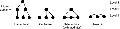
Hierarchical structures have multiple control layers, with distributed decision making between layers, improving robustness, but disturbances significantly reduce performance (Leitão, 2009). An example hierarchical breakdown for assembly uses the final assembler to allocate modules to intermediate sub-assemblers, reducing the complexity of the final assembly process (S. J. Hu et al., 2008; Modrak & Marton, 2012). Hierarchical architectures typically use the same methods as centralised systems within each controlling entity. The traditional method of managing complexity, through simplification and increasing levels of hierarchy, has been shown to perform very poorly compared to alternative structures as complexity and scale increases (Ma et al., 2018).

Centralised systems aim to optimally, or near optimally, satisfy all constraints simultaneously (Scholz-Reiter et al., 2010). There are a variety of mathematical formulations that have been used for solving the assembly problem; however due to computational complexity predominately heuristic algorithms have been proposed (S. J. Hu et al., 2011). To avoid local optima issues, meta-heuristics are used to find optimal/near optimal assembly plans, assembly sequencing and line balancing, popular meta-heuristics are simulated annealing, genetic algorithm and ant-colony optimisation (Wang et al., 2009). Hybrid manufacturing systems aim to combine the benefits of heterarchical systems within a centralised or hierarchical structure; these systems guide or bound distributed decision making but ultimately have a hierarchy of power; an example is fractal manufacturing (Warnecke, 2003).

Heterarchical distributed systems allow low-level decision-making intelligence and autonomy, enabling them to coordinate and interact with each other and the environment (Cantamessa, 1997). There is no active central decision-making or hierarchical/layered structure; many have loosely coupled temporary relationships rather than a predefined and fixed structure. Decentralised structures have been developed for production planning, scheduling and control, to achieve flexibility and fault tolerance that hierarchical systems lack (He et al., 2014), aiming to adapt to highly dynamic variations in product requirements (Shen & Norrie, 1999). Distributed systems, typically through multi-agent systems (MAS) (Shen & Norrie, 1999), have recently investigated rationally bounded learning agents (Vrabič et al., 2018), feature-based manufacturing for distributed CPS (Adamson et al., 2017), distributed collaboration frameworks (Kádár et al., 2018), control for large-scale and complex systems (Quijano et al., 2017) and resource sharing in production networks (Freitag et al., 2015).

Key benefits and criticisms of distributed systems are linked to structure and design principles. Proposed benefits are self-organisation, flexibility and adaptability, fault-tolerance, real-time control, dealing with complex scenarios (Heragu et al., 2002; Ouelhadj & Petrovic, 2009; Shen & Norrie, 1999). Additionally, distributed and typically agent-based systems are increasingly researched to achieve real-time production control (Sahin et al., 2017). Criticisms for distributed systems are suboptimal global solutions, chaotic and unpredictable outcomes, and myopic decision making (Blunck & Bendul, 2016; He et al., 2014; László László Monostori et al., 2014).

There are few fully distributed systems investigated for assembly, despite recent increasing interest and capabilities provided through IoT and CPS technologies. Wang et al. comment that agent-based distributed manufacturing assembly has emerged for adaptive and dynamic process planning (Wang et al., 2009). Additionally, Krüger et al. propose combining decentralised and embedded controllers with machine learning for automation, to control system elements, including robotics, for flexible and reconfigurable assembly lines (Krüger et al., 2017). Antzoulatos et al. propose a MAS framework, using heterarchical with mediator structure, for plug-in/-out reconfigurable assembly resources (Antzoulatos et al., 2017); these intelligent and distributed resources align to the paradigm of CPS (L. L. Monostori et al., 2016). CPS are a network of interacting cyber and physical elements; this connects and enables communication between distributed physical objects (Leitão et al., 2016); and this would facilitate the direct communication required between elements in a distributed control system. IoT technologies provide the low-level capabilities for cyber connectivity of physical objects and has been used in cyber manufacturing to realise advanced analytics for distributed objects (Lee et al., 2016).

Anarchic manufacturing is a fully heterarchical distributed system, where there is no central oversight or control, low-level system elements have decision-making authority and autonomy (Ma et al., 2019a). It combines a free market architecture (Dias & Stentz, 2000) with a permutation of Kádár’s contract net protocol with cost factor adaptation (Kádár & Monostori, 2001) for job to resource contracting. The family of heterarchical distributed systems also contains biological manufacturing systems (Ueda et al., 2006) and rule-based systems (Scholz-Reiter et al., 2010) as well as free market systems. The anarchic manufacturing system is underpinned by emergent synthesis, where individual agents pursue local and personal objectives to solve globally unclear problems (Ueda et al., 2001). Previous studies comparing anarchic manufacturing to centralised systems for independent job manufacturing (no assembly or inter-dependent jobs) have found the anarchic system to be robust to disruption (Ma et al., 2019a), able to embrace complexity, scale and customisation (Ma et al., 2018, 2019b).

3. Anarchic manufacturing for assembly

3.1. Introduction and design principles

Anarchic manufacturing system is adapted for mixed-model assembly scenarios, where jobs are inter-dependent for joining operations and must select a model to fulfil orders. Anarchic manufacturing’s design principles are maintained by retaining dynamic distributed decision making in a free market environment, where agents maximise profitability through competitive behaviour, balk at high prices, are opportunistic with lower prices. Global objectives are aligned via the free market structure by generating demand (orders) and using pricing mechanisms for resource allocation. Extensions to anarchic manufacturing for assembly covered in this paper consider natural team working environments requiring collaboration and group consensus; additionally job agents have decision-making authority over what model or product they become.

Anarchic manufacturing for assembly aims to achieve agility through maximising flexibility in the system, robustness under disturbances, self-coordination and organisation whilst globally realising objectives of fulfilling orders in a complex environment. This will validate and extend research into distributed systems through applying them to a scenario not previously evaluated.

3.2. System structure and mechanisms

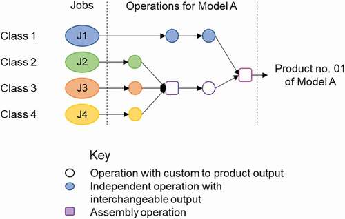
The anarchic manufacturing system fulfils orders by generating demand for the associated model; this influences profitability and subsequent agent decision making. The system consists of jobs, where job i of class c is noted as J_ic and there are a total of n_Job, jobs are processed into products (finished goods and realisation of models) to fulfil customer orders of models, where model k is noted as M_k and there are n_M models, by using resources (machine tools) to complete operations, where resource p of capability j is noted as R_p there are a total of n_R resources. Models have predefined operations that combine different job classes requiring a specific capability and have a nominal duration; these are represented by precedence graphs, see Figure 2 for an example precedence graph and annotations identifying jobs, classes, models and products.

Figure 2. Example precedence graph

Orders for specific models are created periodically and are fulfilled on a FIFO basis by completed products. Models differ but may have common jobs until an operation customises the job to a model; i.e. jobs can fulfil multiple models until the point of model customisation. Following the free market structure, there is a product selling price on fulfilling an order. The selling price informs incomplete jobs of the benefit on fulfilling a specific model and influences job decision making which is profit maximising. The system creates jobs so that there are enough jobs of each class plus a small buffer, in experimentation there are three additional jobs of each class, to fulfil current orders.

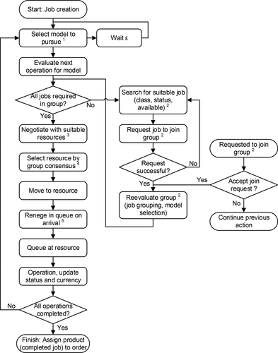
The anarchic manufacturing system for assembly is best described by following a job’s processes. A job decides which model to pursue, it then assesses the next operation for this model and whether additional jobs are required. If so, it will search for jobs and request them in turn to connect. If the request is successful a regrouping process determines, through profit maximisation, which model to pursue and which jobs to group together. Once all required jobs are connected for the next operation, they negotiate with resources individually. As jobs have individual objectives and may prefer different resources, a group consensus method, based on the Borda Count, selects the most suitable resource. A job can renege on arrival to a queue by paying off the job in front. On completing each operation, the job reassesses which model to pursue and on completing all operations for a model, it is assigned to an order. This process is shown in Figure 3; five key decision-making processes and actions highlighted are covered in depth.

Figure 3. Job decision flow chart

3.2.1. Model profitability and selection

A job, on creation and after each operation, selects a model to pursue, Figure 3 note 1, using model profitability in a roulette wheel selection process (Lipowski & Lipowska, 2012), which is socially beneficial to achieve global goals. Roulette wheel selection randomly selects a weighted option, weightings change the probability of selection. This selection process requires calculating the profitability of each model at time t for job i of class c, Pft_ik(t), determined by Equations 1(1) $Pf{t}_{ik}\left(t\right)=FWg{t}_{ik}\left(t\right)\cdot \left(Pr{c}_{ik}\left(t\right)-Cex{p}_{ik}\left(t\right)+5\cdot \left(Dm{d}_k\left(t\right)-Ff{l}_{ck}\left(t\right)\right)\right)$(1) –7(7) $FWg{t}_{ik}\left(t\right)=0.5+0.5\cdot min\left(\frac{Dm{d}_k\left(t\right)}{Ff{l}_{ck}\left(t\right)},2\right)+\sum _{C_c=0}^{n_c}\left(0.5\cdot \left(min\left(\frac{C_k\cdot Dm{d}_k\left(t\right)}{Ff{l}_{ck}\left(t\right)},2\right)-1\right)\right)$(7) . Profitability considers the selling price if job i can still fulfil model k at time t, Prc_ik(t), expected total cost, Cexp_ik(t), which incorporates costs already incurred and currency available, the demand for model k, Dmd_k(t), the number of jobs of the same class fulfilling model k, Ffl_ck(t), and the fulfilment model weighting, FWgt_ik(t), which considers the model demand and fulfilment by all job classes required to complete the model. The profitability of model k for job i at time t is calculated by

(1) $Pf{t}_{ik}\left(t\right)=FWg{t}_{ik}\left(t\right)\cdot \left(Pr{c}_{ik}\left(t\right)-Cex{p}_{ik}\left(t\right)+5\cdot \left(Dm{d}_k\left(t\right)-Ff{l}_{ck}\left(t\right)\right)\right)$(1)

The coefficient of 5 increases the impact between model demand and model fulfilment on decision making. To evaluate the expected cost, a binary function is used to determine whether an operation of capability j is required by job i of class c (J_ic) for model k at time t, O_ickj; given the status of job i, i.e. the number of operations required to fulfil model k given the operations the job has completed.

(2) $O_{ickj}\left(t\right)=\left\{\begin{array}{cc}1& \begin{array}{c}if{J}_{ic}requiresoperationOofcapabilityj\\ tofulfilmodelkattimet\end{array}\\ 0& otherwise\end{array}\right.$(2)

Another binary function is used to determine whether job J is in the group containing job i, J_igrp, at time t.

(3) $J_{Ji}\left(t\right)=\left\{\begin{array}{cc}1& if{J}_J\in J_{igrp}attimet\\ 0& otherwise\end{array}\right.$(3)

The expected total cost considers the expected cost of operations outstanding for the job to complete the product and the cost of operations already incurred and all available currency from jobs in the job group containing job i at time t, J_igrp(t). The expected total cost, Cexp_ik(t), uses the average recent cost of capability j, Cst_j(t), costs already incurred by all jobs in the group, CstHis_igrp (t), and the currency available to job J at time t, Cry_J(t), is calculated as

(4) $Cex{p}_{ik}\left(t\right)=\sum _{O_k=0}^{n_{Ok}}\left(Cs{t}_j\left(t\right)\cdot O_{ickj}\left(t\right)\right)+\sum _{J=0}^{n_{Job}}\left(J_{Ji}\left(t\right)\left(CstHi{s}_{Jgrp}\left(t\right)-Cr{y}_J\left(t\right)\right)\right)$(4)

where O_k is the index of operations required for model k and n_ok is the total number of operations.

A job accounts for the demand for a model and the number of other jobs of the same class aiming to fulfil this model. The number of jobs that are similarly to job i of class c fulfilling model k, Ffl_ck(t), which sums all the model (profitability) weightings of jobs of a particular class and model (i.e. if a job can fulfil multiple models, the model weighting for each model is taken, each are a fraction of and sum to 1), is calculated as

(5) $Ff{l}_{ck}\left(t\right)=\sum _{C_J=C_i\wedge k_J=k_i}\frac{Pf{t}_{Jck}\left(t\right)}{{\sum }_{Pf{t}_{Jck}\left(t\right)\ge 0}Pf{t}_{Jck}\left(t\right)}$(5)

The fulfilment model weighting for job i for model k at time t, FWgt_ik(t), considers the demand for model k and the fulfilment by jobs of the same class c and then adjusts this by the demand and fulfilment by other job of classes required to be joined with for model k. The job uses the weighting to assess the demand fulfilment by the same class, and is influenced heavily by other classes it is required to join with. A binary function defines the job classes required for model k is defined as

(6) $C_k=\{\begin{array}{cc}1& \begin{array}{c}ifclasscisrequiredformodelkand\\ notthesameclassasJobi\end{array}\\ 0& otherwise\end{array}$(6)

The fulfilment model weighting, FWgt_ik(t), considers the demand over fulfilment of a model but bounds these factors between 0 and 2 using the minimum function, it is defined as

(7) $FWg{t}_{ik}\left(t\right)=0.5+0.5\cdot min\left(\frac{Dm{d}_k\left(t\right)}{Ff{l}_{ck}\left(t\right)},2\right)+\sum _{C_c=0}^{n_c}\left(0.5\cdot \left(min\left(\frac{C_k\cdot Dm{d}_k\left(t\right)}{Ff{l}_{ck}\left(t\right)},2\right)-1\right)\right)$(7)

3.2.2. Job connection, grouping and group model selection

If job A requires additional jobs to complete the next operation, it will search for suitable jobs to connect with against class, availability and status criteria; see Figure 3 note 2. Jobs are available if they are not complete products or in operation; therefore, a job is available whilst queuing. A job’s status indicates which operations have been completed. Job A will search for suitable jobs and approach the first, job B, and send job B a request to connect respective groups, Grp_A(t) and Grp_B (t), if the request is accepted a group reevaluation occurs, if unsuccessful job A approaches the next suitable job. Job B will accept the request to connect subject to the scenario; regarding job A and B’s model selection, k, and whether job B has selected and is queuing at a resource, R_B. The acceptance criteria is based on both jobs’ model fulfilment weighting, Ffl_ik(t), which indicates the level of commitment to model k and currency held by each group, Cry_grp; these scenarios and criteria are detailed in Table 1.

Table 1. Job request connection criteria

Scenario at time t	Criteria
$k_A=k_B\wedge R_B=\mathrm{\varnothing }$	$Cr{y}_{grpA}\left(t\right)\cdot Ff{l}_{A{k}_A}\left(t\right)\ge 0.7\cdot Cr{y}_{grpB}\left(t\right)\cdot Ff{l}_{B{k}_B}\left(t\right)$
$k_A\ne k_B\wedge R_B=\mathrm{\varnothing }$	$Cr{y}_{grpA}\left(t\right)\cdot Ff{l}_{A{k}_A}\left(t\right)\ge 1\cdot Cr{y}_{grpB}\left(t\right)\cdot Ff{l}_{B{k}_B}\left(t\right)$
$k_A=k_B\wedge R_B\ne \mathrm{\varnothing }$	$Cr{y}_{grpA}\left(t\right)\cdot Ff{l}_{A{k}_A}\left(t\right)\ge 1.5\cdot Cr{y}_{grpB}\left(t\right)\cdot Ff{l}_{B{k}_B}\left(t\right)$
$k_A\ne k_B\wedge R_B\ne \mathrm{\varnothing }$	$Cr{y}_{grpA}\left(t\right)\cdot Ff{l}_{A{k}_A}\left(t\right)\ge 2\cdot Cr{y}_{grpB}\left(t\right)\cdot Ff{l}_{B{k}_B}\left(t\right)$

Where a job’s model fulfilment weighting, Ffl_ik(t), determines the proportional weighting of model k by profitability against all models for job i, is defined as

(8) $Ff{l}_{ik}\left(t\right)=\frac{Pf{t}_{ik}\left(t\right)}{{\sum }_{Pf{t}_{ik}\left(t\right)\ge 0}Pf{t}_{ik}\left(t\right)}$(8)

If job A satisfies the connecting request criteria all jobs connected to jobs A and B are re-evaluated together. On reevaluation a model is selected and the most suitable jobs for it are grouped (both using currency held multiplied by model fulfilment weighting), this is repeated until all jobs are grouped together and each have a model to pursue. This process is conducted by a nominated job in the group for administrative purposes only, there is no bias or benefit. This regrouping process selects the best and most suited jobs, therefore jobs can dynamically change groups up until they are operated on; changing is determined by how attractive the offer is in the scenario.

3.2.3. Job to resource negotiation

A job, after connecting with all required jobs, will each negotiate the next operation with resources, by their own objectives; this relates to the process in Figure 3 note 3. The anarchic negotiation protocol follows that of Ma et al.’s with a few adjustments (Ma et al., 2019a); this has the same structure as the contract net protocol (Smith, 1980).

A job will communicate with applicable (capable) resources and invite them to tender, the job evaluates a threshold it is willing to spend on this next operation; by proportioning the combined currency of the group against the value of the next operation over the value of all operations remaining to complete the model. Additionally, the job calculates an inter-bidding round increment as a small proportion of the threshold. Each resource invited to tender evaluates an initial bid and inter-bid reduction. The resource’s initial bid for bid round n for resource p of capability j at time t, β_pjn (t), is a function of recent average cost of capability j, Cst_j (t), recent utilisation, ω_p (t), utilisation weighting, U_p, total queue length, Qtot_p(t), which is a combination of assigned jobs, Qasg_p(t), and expected queue length, Qexp_p(t); and is defined as

(9) ${\beta }_{pjn}=1.1\cdot Cs{t}_j\left(t\right)\cdot \left(U_p{\omega }_p\left(t\right)+\frac{\left(1-U_p\right)Qto{t}_p\left(t\right)}{Q_{jutil}}\right)$(9)

where 1.1 is an initial surplus value, and utilisation, ωp(t), and total queue length, Qtot_p(t), is weighted 0.3:0.7, and Q_jutil is the queue size of resources with capability j required to meet full utilisation over the planning time horizon. Total queue length, considering queue already assigned and the expected queue, is defined as

(10) $Qto{t}_p\left(t\right)=Qas{g}_p\left(t\right)+Qex{p}_p\left(t\right)$(10)

To count the number of resources of a capability, resource R with capability j, R_Rj, is represented as a binary value:

(11) $R_{Rj}=\{\begin{array}{cc}1& ifresourcephascapabilityj\\ 0& otherwise\end{array}$(11)

The expected queue is an estimated number of operations in the current pool of jobs requiring capability j, considering how many operations of capability j are required for a job of class c to fulfil model k, O_ckj, and the number of jobs of class c fulfilling model k, Ffl_ck(t), as defined in Equation 5(5) $Ff{l}_{ck}\left(t\right)=\sum _{C_J=C_i\wedge k_J=k_i}\frac{Pf{t}_{Jck}\left(t\right)}{{\sum }_{Pf{t}_{Jck}\left(t\right)\ge 0}Pf{t}_{Jck}\left(t\right)}$(5) . The expected queue length, Qexp_p(t), is defined as

(12) $Qex{p}_p\left(t\right)=0.5\cdot \frac{{\sum }_{j=j_p}Ff{l}_{ck}\left(t\right)\cdot O_{ckj}}{{\sum }_{R=0}^{n_R}{R}_{Rj}}$(12)

The factor of 0.5 is taken, as holistically jobs are expected to be halfway through production.

The resource’s inter-bid round reduction, Red_p(t), is bounded between 1 and 10 and is a function of recent bid success, τ_p(t), and actual job queue over expected job queue; this is defined as

(13) $Re{d}_p\left(t\right)=5\cdot \left(2-{\tau }_p\left(t\right)+\frac{Qas{g}_p\left(t\right)}{Qex{p}_p\left(t\right)}\right)$(13)

After job and resources have evaluated their bidding values, the job evaluates and records all bids, and will continue bidding rounds until a bid received is below the job’s threshold or the maximum of five rounds is reached. Between bidding rounds a job increases its threshold by the increment and resources lower their bids by reduction, Red_p(t). If five bidding rounds have been exceeded the job records the resource bids from the last round and will retender after a short waiting time if another job in its group has not successfully negotiated with resources.

3.2.4. Job group consensus, resource selection

A group of jobs must decide which resource to select, relating to Figure 3 note 4; however, with different objectives they may have different preferences; a currency weighted Borda Count method (Zahid & De Swart, 2015) is used to select a single option. The Borda Count gives points for each voting participant to candidates in rank order; for m candidates the highest ranked receives m votes and the second m–1 votes, etc. The highest scoring candidate resource is selected by multiplying the job’s (voter’s) currency held and the Borda Count score for all jobs. The lowest negotiated price for the resource by any job is taken.

3.2.5. Job renege in queue

On arrival to a resource queue a job (A), or the administrative job, will renege if possible to skip the queue; at note 5 for Figure 3. Reneging is to go back on an agreement, here it is used to negotiate with other jobs to take their place in the queue for a negotiate cost. The remaining joint currency after negotiation, threshold less operation cost, is used to pay off the next job (B) in the queue. Job B calculates a payoff queue-skipping price and will allow job A to go ahead in the queue if the payoff price is below job A’s remaining currency. Job B’s queue-skipping price is the original negotiation threshold plus time (min) since the first tender less the operation cost.

4. Experimentation

Experimentation investigated two mixed-model assembly scenarios, idealised balanced production and dynamic bottlenecks, comparing the anarchic manufacturing system and two centralised systems. These two idealised scenarios are suitable to extend knowledge as there have been no reported experimental studies into distribute systems for assembly. The two comparative centralised systems both used a push model but differing cell structures.

The general mixed-model assembly production planning and control problem investigated here fulfils orders of predetermined models (products), orders are periodically created and randomly assigned a model. Each model has a fixed precedence graph, see Figure 2 for an example, where orders are fulfilled by jobs of particular classes that undertake a sequence of operations to become products. If the production planning and control system allows, jobs may be used for different orders and even products, if the job (or subsystem) has not been customised to a model for the latter.

Metrics of work in progress (WIP) and order lead time were recorded and analysed for both experiments, which allowed for simulation ramp-up and long run behaviour. WIP indicates the system cash position and relative production efficiency, order lead time indicates fulfilment speed and service level. Agent-based models were created, enabling for independent decision making for each element, and simulations used 50 runs for each parameter setting to achieve a high level of confidence. AnyLogic was used for efficient agent-based simulation modelling.

The experimental setup and input data were fabricated to reduce unnecessary noise and to focus on comparing anarchic against centralised systems in a generalised manufacturing environment. Inputs directly reflecting industry can obscure results, through unnecessary real-world representation or industry-specific problems. These idealised scenarios are most suitable to evaluate the holistic feasibility of anarchic manufacturing and distributed structures.

4.1. Comparative centralised system

The two comparative centralised systems used a push model, with three levels of hierarchy but different cell structures; see Figure 4 for system illustrations. A push system was selected over pull to manage increasing variation in mixed-model production. Krishnamurthy et al. state pull strategies are fundamentally handicapped for manufacturing facilities that produce different products with distinct demands and/or processing requirements (Krishnamurthy et al., 2004).

Figure 4. Centralised systems structures

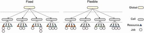
In the fixed system cells contained one of each resource type and cells manufactured all jobs for an order. Whereas the flexible system had a flow shop structure, cells contained all resources of a particular capability. The global coordinator reassigned jobs to capability cells for each operation. Both systems used the earliest due date (EDD) dispatch rule (heuristic) to allocate jobs to cell/resource. Both systems used a push system and following material resource planning (MRP) practice, jobs (or materials) are assigned to an order and cannot transfer to another (Lewis & Slack, 2003).

For both centralised systems no line balancing was required or traditional assembly sequencing. Experiment setup created nominally balanced production with flexible in cell routing; rather than rigid assembly lines of sequential workstations.

4.2. Balanced production

4.2.1. Introduction

A balanced production experiment evaluated anarchic against centralised systems in an idealised state with increasing levels of drift. Although manufacturers aim to minimise drift, for mixed-model assembly lines it will be almost impossible to balance the line properly, due to differing model characteristics (S. J. Hu et al., 2011), this is extended by stochastic operation durations. This nominally balanced production scenario, with increasing levels of drift, will clearly indicate performance regardless of line balancing.

4.2.2. Method

Both systems aim to fulfil orders for three models by performing joining and independent operations on jobs. There are 16 resources (machine tools), 4 of each capability, there are 3 capabilities (A, B, C) for independent operations and 1 capability (Z) for joining. Orders arrive at a constant rate, maintaining 60% utilisation, are randomly assigned a model against a split of 0.4:0.4:0.2, see Table 2 for a summary of fixed parameters. There are no additional resources required or work in progress restrictions, movement durations are very small relative to operation durations.

Table 2. Balanced production fixed parameters

Parameter	Value
No. resources	16 MTs
No. capabilities	4 (4 of each)
No. cells (central fixed and flexible only)	4 cells
Nominal utilisation rate	60%
No. models (weighted split)	3 (0.4:0.4:0.2)
Average operating time/product	160 min
Average operation duration	20 min

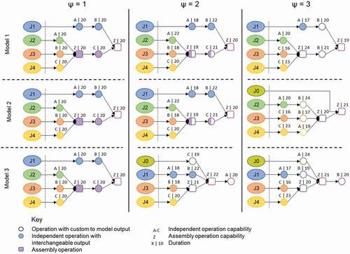
The experiment increases levels of drift, both structurally in parameter, ψ, and through stochastic operation durations, δ; both parameters have three levels. As structural drift, ψ, increases nominal operation duration is more varied, model precedence structures increasingly diverge and job customisation to a particular model is earlier (reducing job interchangeability between models). This parameter progression is shown in Figure 5, displaying model precedence graphs with model customisation, operation capability and nominal durations. To maintain nominally balanced production, all models require each capability twice. The second parameter stochastic operation durations, δ, vary durations against a uniform random distribution, increasing from 0 to 0.25 and 0.5.

Figure 5. Balanced production, structural drift precedence graphs

4.2.3. Results

The experiment results, shown in Figure 6 for WIP jobs with a 95% confidence interval, Figure 7 for order lead time and Table 3 for lead time population splits, directly compare the three systems. The 95% confidence interval for Figures 6 and 9 is very narrow and appears as a line in some plots, these areas when not overlapping with a mean line indicate that the results are different at 95% confidence interval. WIP jobs results indicate anarchic manufacturing is significantly better when all models are identical, ψ = 1, additionally for moderate structural drift, ψ = 2, all systems perform similarly; at both levels the anarchic system maximises flexibility. For ψ = 3, the anarchic system’s poor performance arises from structural inflexibility, preventing jobs model transferring due to earlier customisation to model. Decision making mechanisms, currency levels and costs were not optimised, these hindered jobs from assessing profitability effectively causing some to go beyond the point of customisation before there was sufficient demand. For most parameter levels, the fixed system’s performance was worse than the centralised flexible system. The flexible centralised system performed consistently by prioritising affectively and reduce waiting time for co-dependent jobs. The fixed system represents a hierarchical structure, with siloed cells that do not communicate; whereas the flexible can effectively manage all resources; a cell manages all interchangeable resources simultaneously. The increasing stochasticity of operation durations, δ, has little impact on system performances compared to structural drift.

Figure 6. Balanced production, WIP job results

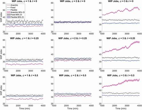
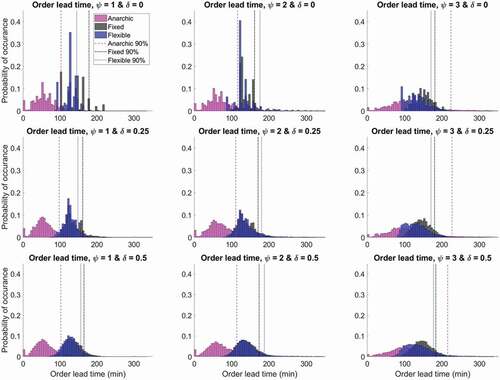
Table 3. Balance production, order lead time population split

Order lead time		ψ = 1			ψ = 2			ψ = 3
		50%	75%	90%	50%	75%	90%	50%	75%	90%
δ = 0	Anarchic	55.4	75.1	102.5	67.4	88.1	115.7	105.5	146.7	223.8
	Flexible	125.6	139.4	144.9	124.0	140.0	175.6	128.3	150.3	170.6
	Fixed	144.8	161.5	178.2	128.3	151.4	161.1	149.5	164.8	180.8
δ = 0.25	Anarchic	55.2	73.7	97.7	64.5	86.7	110.9	102.9	148.2	227.0
	Flexible	125.2	137.3	148.1	133.3	150.7	179.8	127.9	149.8	170.6
	Fixed	129.1	150.3	161.2	133.4	153.7	170.6	145.9	163.4	179.9
δ = 0.5	Anarchic	56.5	76.8	102.1	64.4	88.3	113.7	106.4	146.5	214.9
	Flexible	127.7	141.4	155.8	137.1	156.6	187.3	130.7	154.5	177.2
	Fixed	132.5	149.4	164.6	137.0	155.4	173.3	147.0	165.3	183.2

Analysing order lead time results in Figure 7 and Table 3, anarchic manufacturing outperforms both centralised systems for the majority of orders in all scenarios. The anarchic system, for ψ = 1 & 2, significantly outperforms the push systems for all orders; even for moderate structural drift and reduced flexibility for ψ = 2. For ψ = 3, the anarchic system has a superior performance for the initial 75% of orders, as shown in Table 3, but a longer tail of prolonged order lead times. This is because anarchic systems demonstrate anticipatory behaviour, guided by model profitability, whilst utilising dynamic demand oriented decision making; producing a strong global result despite the heavily criticised myopic decision making (although reduced as jobs maximise lifetime profitability). The fixed and flexible system performances mimic that of WIP jobs performance, with consistency at all parameter levels. It is unknown why for ψ = 2 the flexible system consistently performs worse. Operation duration stochasticity does not significantly impact performance; at reduced stochasticity levels all systems have spikes, which is due to repeated identical sequences.

Figure 7. Balanced production, order lead time results

4.3. Dynamic bottleneck production

4.3.1. Introduction

Bottlenecks can significantly reduce productivity, many current bottleneck detection schemes focus on long-term detection, typically evaluated analytically or through simulation; however, short-term bottleneck detection is increasingly important in operations management (Li et al., 2009). Short-term dynamic bottlenecks are harder to manage and require process control techniques. The experiment created dynamic bottlenecks by drastically increasingly one operation duration, of a different capability, for each model.

4.3.2. Method

This experiment adapted the previous experiment for balanced production, evaluated in Section 4.2, at ψ = 2 and δ = 0.25. Table 4 summaries the fixed parameter settings, notably utilisation increased to 80% (by increasing order arrival rate, adjusted for the extended operation), and order model split is a third each. Average and total model operation durations change by variable parameter and have been omitted.

Table 4. Dynamic bottleneck fixed parameters

Parameter	Value
No. machine tools	16 MTs
No. capabilities	4 (4 MTs of each)
No. cells (central fixed and flexible only)	4 cells
Nominal utilisation rate	80%
No. models (order split between models)	3 (0.33:0.33:0.33)

The experiment increases the severity of the bottleneck by increasing the duration of the single extended operation; this variable parameter is denoted as γ. A dynamic bottleneck between capabilities is ensured by extending a different capability for each model. Figure 8 shows the three model precedence graphs, the extended operation duration is marked ‘XX’ and durations are detailed in Table 5.

Figure 8. Dynamic bottleneck precedence graphs

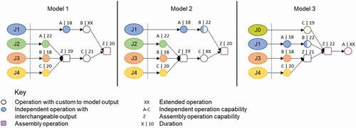
Table 5. Dynamic bottleneck variable parameter

Parameter level	Extended operation duration (min)	Proportion of extended operation of whole process (%)
γ = 1	50	14
γ = 2	75	20
γ = 3	100	25

4.3.3. Results

Results from dynamic bottleneck production are shown in Figure 9 for WIP jobs, Figure 10 for order lead time and Table 6 for order lead time population splits. WIP jobs results, displayed in Figure 9 with a 95% confidence interval, clearly shows the flexible system is best and the anarchic has a similar but slightly worse performance at all parameter levels. The centralised fixed system, with isolated hierarchical cells, performs poorly and for γ = 2 the system is unstable; instability is evident from a continuously increasing trend. All systems are unstable at γ = 3.

Figure 9. Dynamic bottleneck production, WIP jobs results

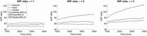
Table 6. Dynamic bottleneck, order lead time population split

Order lead time	γ = 1			γ = 2			γ = 3
	50%	75%	90%	50%	75%	90%	50%	75%	90%
Anarchic	136.3	174.8	223.7	186.2	240.8	304.0	246.3	320.4	399.4
Flexible	181.8	208.1	236.7	229.3	270.4	316.7	293.0	357.5	425.7
Fixed	219.6	250.9	281.2	325.0	385.3	641.9	452.7	548.1	642.0

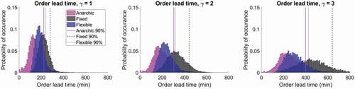
Anarchic systems have superior performance at all levels for order lead time. Order lead times increase as γ increases for all systems, with the anarchic system performing best at all population splits, despite a longer tail than centralised flexible systems. This superior order lead time, improving service level, can be highly attractive to manufacturers. Additionally, it demonstrates the anarchic system’s robustness to unforeseen disruption through its ability to manage short-term dynamic bottlenecks.

Figure 10. Dynamic bottleneck production, order lead time

5. Discussion

5.1. Anarchic manufacturing for assembly

The assembly scheduling and control problem extends independent job manufacture through a coordination problem, assigning jobs to join once all preceding operations have been fulfilled. The anarchic manufacturing system, in the two experiments have demonstrated the ability to resolve this coordination problem in a purely distributed manner. The lack of global coordination in distributed systems is argued for the use of mediators and hybrid systems (Blunck & Bendul, 2016); hybrid systems use a hierarchical structure with distributed decision making (He et al., 2014). However, in this paper inter-job cooperation is achieved using the anarchic manufacturing’s design principles by maintaining free market competition and profit maximisation, fulfilling global objectives met; efficiently delivering orders in a short lead time. The balanced production experiment, covered in Section 4.2, demonstrates that regardless of line balancing activities, mixed-model assembly can effectively be fulfilled through anarchy and distributed systems.

The balanced production experiment demonstrates that the anarchic system can fulfil assembly production whilst maximising flexibility in the system. At lower levels of structural drift, most notably for late model customisation, the anarchic system outperformed centralised systems for both WIP jobs and order lead time. Good order lead time was maintained at higher levels of structural drift, however WIP jobs was poor as reduced flexibility hindered the anarchic system. The dynamic bottleneck production experiment demonstrated the anarchic system’s ability to adapt to disruption, as degradation in performance was in line with the centralised flexible system, which operated as a flow shop. Order lead times, although superior for most orders, had a large distribution; this is undesirable for some manufacturers. However, a more aggressive demand and priority oriented pricing structure will likely resolve this and cut the long tail. This would be achieved by advertising an increased selling price of a highly demanded model to influence job decision making, whilst maintaining the anarchic/distributed structure.

The anarchic manufacturing system’s maximising flexibility trait, through inter-changeable jobs/subsystems and discussed in Section 5.2, could entail that new permutations of existing models can easily be fulfilled without system re-planning. Mixed-model assembly lines typically produced variants from a platform (Battini et al., 2009). An agent’s fulfilment by profitability would indicate suitability for higher-level business decisions on product mix and appropriate pricing as the anarchic system’s free market and profitability-oriented mechanisms directly relate to business objectives.

This research aligns to previous studies; this includes conclusions drawn by Bocella et al., their comparison of centralised against distributed systems concluded that distributed systems were more flexible in response to dynamic and stochastic environments, including failures (Boccella et al., 2020). Additionally, Tochev et al. found that under dynamic scenarios with failures the distributed system was more flexible in managing disruption compared to centralised systems (Tochev et al., 2018). Myopia is a key criticism of distributed systems (Bendul & Blunck, 2019); this research has exhibited the downfalls of this myopia when production constraints limit the system flexibility. However, it is shown that the agility of the system can overcome myopia when production constraints do not impede flexible production. Although these previous studies have similar conclusions, they have not indicated how their systems could be adapted to assembly or mixed-model production, therefore a direct comparison between research studies cannot be made.

Several distributed system traits are exhibited during experimentation, agility and flexibility, self-healing and myopic decision making; these are discussed below.

5.2. Agility and maximising flexibility

The balanced production experiment increases structural drift and reduces available flexibility in the mixed-model assembly system. It is evident that the flexible centralised system maintains performance; however, the anarchic maximises the flexibility available at the reduced drift and high flexibility scenarios. Centralised systems were unable to maximise flexibility available as on aligning to MRP principles the jobs (materials) are assigned an order and cannot change at any point during production. The anarchic manufacturing system’s dynamic decision making for jobs at all stages of production allows for an agile and adaptive delayed decision making; rather than being tied to a specific order from creation.

The anarchic system maximises flexibility by embracing complexity, the less restricted and more complex the system is the more effective flexibility becomes. Following an entropic view to complexity, as the number of options and selection choices increase the more complex the system is (Elmaraghy et al., 2012). The anarchic system has its limits, as seen in the balanced production experiment when structural drift was high at ψ = 3; when earlier customisation limited flexibility, the system’s early decisions based on uncertain information were binding and prevented adaptability to the new scenario. The centralised push systems manage complexity through simplification and structure by assigning jobs an order on creation. The flexible system is effective for all experimental parameter levels, but limits its performance; the fixed system with an hierarchical cells structure performs reasonably well until it faces disruptions, as observed in dynamic bottleneck production in section 4.3.

5.3. Self-healing system

The anarchic manufacturing system exhibits robust self-healing characteristics against dynamic and unforeseen disturbances, as shown in the dynamic bottleneck experiment in section 0. Bottlenecks can significantly impact productivity, even in flexibly structured systems. The anarchic system was able to reallocate operations away from the bottleneck resource to directly interchangeable resources just as effectively as a centralised flexible system that manages all interchangeable resources concurrently. This was observed through similar rates at which WIP jobs, in Figure 9, and order lead time, in Figure 10, increased for the two systems. This aligns to self-organising and fault-tolerant characteristics proposed for distributed systems (Heragu et al., 2002), and reinforcing previous conclusions (Leitão, 2009; Ma et al., 2019a).

5.4. Reducing myopic decision making

Myopic decision making is a key criticism of distributed systems (He et al., 2014), where short-sighted decisions result in globally suboptimal outcomes. The anarchic manufacturing system for assembly has adapted agent decision making to maximise lifetime profitability; demand impacts a product’s selling price and reported recent costs indicate profitability for selecting one model over another. This lifetime profit maximisation is an effective alternative to other myopic decision making counter measures; re-introducing hierarchy and altering competitive behaviour are likely to impede emergent behaviour (Blunck & Bendul, 2016). Lifetime profitability maximisation is a complex decision with highly uncertain outcomes; the environment is likely to change over the course of a job agent’s lifetime. When an early decision was forced, in balanced production at ψ = 3, it impedes agent and global outcomes as agents cannot impact their early decision making.

For flexible scenarios, with late job to model customisation that allow agile systems to maximise flexibility, the impact of myopic decision making is reduced; through delayed and dynamic decision making throughout an agent’s life. However, as shown in the balanced production experiment with reduced flexibility, at ψ = 3, early decisions significantly impact outcome, evident through very high WIP jobs in Figure 6. The lack of global coordination has impacted performance of the anarchic manufacturing system in this uncertain and inflexible environment.

6. Conclusion

The mixed-model production planning and control assembly problem is evaluated comparing anarchic manufacturing to centralised systems. The assembly problem uses multiple jobs that join to form a product, requiring inter-job coordination. Anarchic manufacturing is a distributed system, based on free market principles, and has been successfully applied to the mixed-model assembly problem. Experiments evaluated an idealised balanced production and dynamic bottleneck scenarios and found the anarchic system is superior when it can use complexity to its advantage through maximising flexibility. Additionally, dynamic bottleneck experimentation, that evoked unforeseen disruption, validated previous assertions and studies for the robustness and self-healing nature of distributed systems. The anarchic manufacturing system was able to fulfil mixed-model assembly production, and even exceeded centralised performance under certain circumstances. Several desirable anarchic manufacturing traits were observed; these include agility and maximising flexibility, self-healing and reduced myopic decision making.

There are some limitations to this research, most significantly due to the idealised scenarios used and experiment variables. Idealised scenarios were used to establish a baseline relative performance of the anarchic against centralised systems; however, this cannot be translated directly to industry without further research. Contextual factors beyond those modelled would be required before industrial consideration. Furthermore, the scope of experimentation is relatively narrow to the range of scenarios presented in industry.

This research, by finding that a distributed system can effectively be applied to the assembly problem, impacts both academia and industry. For academia some theorised benefits of distributed systems are realised for assembly scenarios, indicating value in further research into the field. Additionally, the case for free market-based systems is strengthened due to their adaptability to different scenarios. There is still relevance to industry despite the immature state of research into distributed systems for assembly. Industrial applications with an assembly or collaboration problem could in the future benefit from distributed systems as complexity and the need for flexibility rise, particularly when ‘simplify to improve’ is a significant hindrance.

The implications from the findings in this paper suggest that anarchic and distributed systems can be used for assembly, where there is a fundamental coordination problem that extends decision-making processes beyond an individual agent. Future work shall evaluate to what extent can assembly benefit from distributed systems, capitalising on distributed system’s reported traits. This will consider how improving agility and flexibility will impact assembly performance, most notably for increasing number of models and their variability and thereby increasing complexity. Improved responsiveness of distributed systems could challenge the existing methods of fulfilling mixed-model assembly which are rigidly bound in sequencing of assembly lines. Additionally, future work will consider the managerial and business impacts through a multi-disciplined study.

Declaration of interests

The authors declare that they have no known competing financial interests or personal relationships that could have appeared to influence the work reported in this paper.

Acknowledgments

The work has been funded by the Engineering and Physical Sciences Research Council (EPSRC), grant reference EP/N509619/1.

Additional information

Funding

This work was supported by the Engineering and Physical Sciences Research Council Doctoral Training Programme [EP/N509619/1].

References

- Adamson, G., Wang, L., & Moore, P. (2017). Feature-based control and information framework for adaptive and distributed manufacturing in cyber physical systems. Journal of Manufacturing Systems, 43(2), 305–315. https://doi.org/https://doi.org/10.1016/j.jmsy.2016.12.003
- Antzoulatos, N., Castro, E., De Silva, L., Rocha, A. D., Ratchev, S., & Barata, J. (2017). A multi-agent framework for capability-based reconfiguration of industrial assembly systems. International Journal of Production Research, 55(10), 2950–2960. https://doi.org/https://doi.org/10.1080/00207543.2016.1243268
- Asadi, N., Jackson, M., & Fundin, A. (2016). Drivers of complexity in a flexible assembly system- A case study. Procedia CIRP, 41, 189–194. https://doi.org/https://doi.org/10.1016/j.procir.2015.12.082
- Battini, D., Faccio, M., Persona, A., & Sgarbossa, F. (2009). Balancing-sequencing procedure for a mixed model assembly system in case of finite buffer capacity. International Journal of Advanced Manufacturing Technology, 44(3–4), 345–359. https://doi.org/https://doi.org/10.1007/s00170-008-1823-8
- Bendul, J. C., & Blunck, H. (2019). The design space of production planning and control for industry 4.0. Computers in Industry, 105, 260–272. https://doi.org/https://doi.org/10.1016/j.compind.2018.10.010
- Blunck, H., & Bendul, J. (2016). Controlling myopic behavior in distributed production systems - A classification of design choices. Procedia CIRP, 57, 158–163. https://doi.org/https://doi.org/10.1016/j.procir.2016.11.028
- Boccella, A. R., Centobelli, P., Cerchione, R., Murino, T., & Riedel, R. (2020). Evaluating centralized and heterarchical control of smart manufacturing systems in the era of industry 4.0. Applied Sciences (Switzerland), 10(3),755. https://doi.org/https://doi.org/10.3390/app10030755
- Bock, S., Rosenberg, O., & Brackel, T. V. (2006). Controlling mixed-model assembly lines in real-time by using distributed systems. European Journal of Operational Research, 168(3), 880–904. https://doi.org/https://doi.org/10.1016/j.ejor.2004.07.035
- Boysen, N., Fliedner, M., & Scholl, A. (2009). Sequencing mixed-model assembly lines: Survey, classification and model critique. European Journal of Operational Research, 192(2), 349–373. https://doi.org/https://doi.org/10.1016/j.ejor.2007.09.013
- Cantamessa, M. (1997). Agent-balsed modeling and management of manufacturing systems. Computers in Industry, 34(97), 173–186. https://doi.org/https://doi.org/10.1016/S0166-3615(97)00053-5
- Dias, M. B., & Stentz, A. (2000). A free market architecture for distributed control of a multirobot system. 6th International Conference on Intelligent Autonomous Systems IAS6, Venice, IOS Press. 6, 115–122. Venice, IOS Press.
- Duffie, N. A., & Piper, R. S. (1987). Non-hierarchical control of a flexible manufacturing cell. Robotics and Computer-Integrated Manufacturing, 3(2), 175–179. https://doi.org/https://doi.org/10.1016/0736-5845(87)90099-8
- ElMaraghy, H., Schuh, G., ElMaraghy, W., Piller, F., Schonsleben, S., Tseng, M., & Bernard, A. (2013). Product variety management. CIRP Annals - Manufacturing Technology, 62(62), 629–652. https://doi.org/https://doi.org/10.1016/j.cirp.2013.05.007
- Elmaraghy, W., Elmaraghy, H., Tomiyama, T., & Monostori, L. (2012). Complexity in engineering design and manufacturing. CIRP Annals - Manufacturing Technology, 61(2), 793–814. https://doi.org/https://doi.org/10.1016/j.cirp.2012.05.001
- Emde, S., & Polten, L. (2019). Sequencing assembly lines to facilitate synchronized just-in-time part supply. Journal of Scheduling, 22(6), 607–621. https://doi.org/https://doi.org/10.1007/s10951-019-00606-w
- Freitag, M., Becker, T., & Duffie, N. A. (2015). Dynamics of resource sharing in production networks. CIRP Annals - Manufacturing Technology, 64(1), 435–438. https://doi.org/https://doi.org/10.1016/j.cirp.2015.04.124
- Gyulai, D., Pfeiffer, A., & Monostori, L. (2017). Robust production planning and control for multi-stage systems with flexible final assembly lines. International Journal of Production Research, 55(13), 3657–3673. https://doi.org/https://doi.org/10.1080/00207543.2016.1198506
- He, N., Zhang, D. Z., & Li, Q. (2014). Agent-based hierarchical production planning and scheduling in make-to-order manufacturing system. International Journal of Production Economics, 149, 117–130. https://doi.org/https://doi.org/10.1016/j.ijpe.2013.08.022
- Heragu, S. S., Graves, R. J., Kim, B., & Onge, A. S. (2002). Intelligent agent based framework for manufacturing systems control. IEEE, Trans. Syst. Man. Cybern, 32(5), 560–573. https://doi.org/https://doi.org/10.1109/TSMCA.2002.804788
- Hu, S. J., Ko, J., Weyand, L., Elmaraghy, H. A., Lien, T. K., Koren, Y., … Shpitalni, M. (2011). Assembly system design and operations for product variety. CIRP Annals - Manufacturing Technology, 60(2), 715–733. https://doi.org/https://doi.org/10.1016/j.cirp.2011.05.004
- Hu, S. J., Zhu, X., Wang, H., & Koren, Y. (2008). Product variety and manufacturing complexity in assembly systems and supply chains. CIRP Annals - Manufacturing Technology, 57(1), 45–48. https://doi.org/https://doi.org/10.1016/j.cirp.2008.03.138
- Hu, S. J. (2014). Assembly. In L. Laperrière & G. Reinhart (Eds.), CIRP encyclopedia of production engineering (pp. 50–52). Springer Berlin Heidelberg. https://doi.org/https://doi.org/10.1007/978-3-642-20617-7_6616
- Kádár, B., Egri, P., Pedone, G., & Chida, T. (2018). Smart, simulation-based resource sharing in federated production networks. CIRP Annals, 67(1), 503–506. https://doi.org/https://doi.org/10.1016/j.cirp.2018.04.046
- Kádár, B., & Monostori, L. (2001). Approaches to increase the performance of agent-based production system. https://doi.org/https://doi.org/10.1007/3-540-45517-5_68
- Kampker, A., Deutskens, C., Deutschmann, K., Maue, A., & Haunreiter, A. (2014). Increasing ramp-up performance by implementing the gamification approach. Procedia CIRP, 20(C), 74–80. https://doi.org/https://doi.org/10.1016/j.procir.2014.05.034
- Komaki, G. M., Sheikh, S., & Malakooti, B. (2019). Flow shop scheduling problems with assembly operations: A review and new trends. International Journal of Production Research, 57(10), 2926–2955. https://doi.org/https://doi.org/10.1080/00207543.2018.1550269
- Krishnamurthy, A., Suri, R., & Vernon, M. (2004). Re-examining the performance of MRP and kanban material control strategies for multi-product flexible manufacturing systems. International Journal of Flexible Manufacturing Systems, 16(2), 123–150. https://doi.org/https://doi.org/10.1023/B:FLEX.0000044837.86194.19
- Krüger, J., Wang, L., Verl, A., Bauernhansl, T., Carpanzano, E., Makris, S., … Pellegrinelli, S. (2017). Innovative control of assembly systems and lines. CIRP Annals, 66(2), 707–730. https://doi.org/https://doi.org/10.1016/j.cirp.2017.05.010
- Lee, J., Bagheri, B., & Jin, C. (2016). Introduction to cyber manufacturing. Manufacturing Letters, 8, 11–15. https://doi.org/https://doi.org/10.1016/j.mfglet.2016.05.002
- Leitão, P. (2009). Agent-based distributed manufacturing control: A state-of-the-art survey. Engineering Applications of Artificial Intelligence, 22(7), 979–991. https://doi.org/https://doi.org/10.1016/j.engappai.2008.09.005
- Leitão, P., Colombo, A. W., & Karnouskos, S. (2016). Industrial automation based on cyber-physical systems technologies: Prototype implementations and challenges. Computers in Industry, 81, 11–25. https://doi.org/https://doi.org/10.1016/j.compind.2015.08.004
- Lewis, M., & Slack, N. (2003). Operations management: Critical perspectives on business and management. Routledge. https://books.google.co.uk/books?id=cGzxgjWUkaYC
- Li, L., Chang, Q., & Ni, J. (2009). Data driven bottleneck detection of manufacturing systems. International Journal of Production Research, 47(18), 5019–5036. https://doi.org/https://doi.org/10.1080/00207540701881860
- Lipowski, A., & Lipowska, D. (2012). Roulette-wheel selection via stochastic acceptance. Physica A: Statistical Mechanics and Its Applications, 391(6), 2193–2196. https://doi.org/https://doi.org/10.1016/j.physa.2011.12.004
- Ma, A., Nassehi, A., & Snider, C. (2018). Anarchic manufacturing and mass customisation. In Cambridge International Manufacturing Symposium (pp. 1–17). Cambridge, UK: IfM. https://doi.org/https://doi.org/10.1080/00207543.2018.1521534
- Ma, A., Nassehi, A., & Snider, C. (2019a). Anarchic manufacturing. International Journal of Production Research, 57(8), 2514–2530. https://doi.org/https://doi.org/10.1080/00207543.2018.1521534
- Ma, A., Nassehi, A. and Snider, C., 2019b. Embracing complicatedness and complexity with Anarchic Manufacturing. Procedia Manufacturing, 28, pp.51–56.
- Modrak, V., & Marton, D. (2012). Modelling and complexity assessment of assembly supply chain systems. Procedia Engineering, 48, 428–435. https://doi.org/https://doi.org/10.1016/j.proeng.2012.09.536
- Monostori, L., Kádár, B., Bauernhansl, T., Kondoh, S., Kumara, S., Reinhart, G., Sauer, O., Schuh, G., Sihn, W., & Ueda, K. (2016). Cyber-physical systems in manufacturing. CIRP Annals - Manufacturing Technology, 65(2), 621–641. https://doi.org/https://doi.org/10.1016/j.cirp.2016.06.005
- Monostori, L., Valckenaers, P., Dolgui, A., Panetto, H., Brdys, M., & Csáji, B. C. (2014). Cooperative control in production and logistics. IFAC Proceedings Volumes (IFAC-papersonline), 19(3), 4246–4265. https://doi.org/https://doi.org/10.1016/j.arcontrol.2015.03.001
- Ouelhadj, D., & Petrovic, S. (2009). A survey of dynamic scheduling in manufacturing systems. Journal of Scheduling, 12(4), 417–431. https://doi.org/https://doi.org/10.1007/s10951-008-0090-8
- Quijano, N., Ocampo-Martinez, C., Barreiro-Gomez, J., Obando, G., Pantoja, A., & Mojica-Nava, E. (2017). The role of population games and evolutionary dynamics in distributed control systems: The advantages of evolutionary game theory. IEEE Control Systems, 37(1), 70–97. https://doi.org/https://doi.org/10.1109/MCS.2016.2621479
- Sahin, C., Demirtas, M., Erol, R., Baykasoğlu, A., & Kaplanoğlu, V. (2017). A multi-agent based approach to dynamic scheduling with flexible processing capabilities. Journal of Intelligent Manufacturing, 28(8), 1827–1845. https://doi.org/https://doi.org/10.1007/s10845-015-1069-x
- Schenk, M., Wirth, S., & Müller, E. (2009). Factory planning manual: Situation-driven production facility planning. Springer Berlin Heidelberg. https://books.google.co.uk/books?id=EqzmcXBOcbAC
- Scholz-Reiter, B., Rekersbrink, H., & Görges, M. (2010). Dynamic flexible flow shop problems - Scheduling heuristics vs. autonomous control. CIRP Annals - Manufacturing Technology, 59(1), 465–468. https://doi.org/https://doi.org/10.1016/j.cirp.2010.03.030
- Shen, W., Hao, Q., Yoon, H. J., & Norrie, D. H. (2006). Applications of agent-based systems in intelligent manufacturing: An updated review. Advanced Engineering Informatics, 20(4), 415–431. https://doi.org/https://doi.org/10.1016/j.aei.2006.05.004
- Shen, W., & Norrie, D. H. (1999). Agent-based systems for intelligent manufacturing: A State-of-the-Art survey. Knowledge and Information Systems, 1(2), 129–156. https://doi.org/https://doi.org/10.1007/BF03325096
- Smith, R. G. (1980). The contract net protocol: High-level communication and control in a distributed problem solver. IEEE TRansaction on Computer, C–29, 12, 1104–1113. doi:https://doi.org/10.1109/TC.1980.1675516.
- Tharumarajah, A. (2001). Survey of resource allocation methods for distributed manufacturing systems. Production Planning and Control, 12(1), 58–68. https://doi.org/https://doi.org/10.1080/09537280150203988
- Tochev, E., Pfifer, H., & Ratchev, S. (2018). A comparison of centralised and decentralised scheduling methods using a simple benchmark system. IFAC-PapersOnLine, 51(11), 1287–1292. https://doi.org/https://doi.org/10.1016/j.ifacol.2018.08.355
- Ueda, K., Kito, T., & Fujii, N. (2006). Modeling biological manufacturing systems with bounded-rational agents. CIRP Annals - Manufacturing Technology, 55(1), 469–472. https://doi.org/https://doi.org/10.1016/S0007-8506(07)60461-2
- Ueda, K., Markus, A., Monostori, L., Kals, H. J. J., & Arai, T. (2001). Emergent synthesis methodologies for manufacturing. CIRP Annals - Manufacturing Technology, 50(2), 535–551. https://doi.org/https://doi.org/10.1016/S0007-8506(07)62994-1
- Vrabič, R., Kozjek, D., Malus, A., Zaletelj, V., & Butala, P. (2018). Distributed control with rationally bounded agents in cyber-physical production systems. CIRP Annals, 67(1), 507–510. https://doi.org/https://doi.org/10.1016/j.cirp.2018.04.037
- Wang, L., Keshavarzmanesh, S., Feng, H. Y., & Buchal, R. O. (2009). Assembly process planning and its future in collaborative manufacturing: A review. International Journal of Advanced Manufacturing Technology, 41(1–2), 132–144. https://doi.org/https://doi.org/10.1007/s00170-008-1458-9
- Warnecke, H. J. (2003). Fractal Company—A Revolution in Corporate Culture. In Manufacturing Technologies for Machines of the Future (pp. 63-85). Springer, Berlin, Heidelberg.
- Zahid, M. A., & De Swart, H. (2015). The borda majority count. Information Sciences, 295, 429–440. https://doi.org/https://doi.org/10.1016/j.ins.2014.10.044