Improved GRU prediction of paper pulp press variables using different pre-processing methods

ABSTRACT

Predictive maintenance strategies are becoming increasingly more important with the increased needs for automation and digitalization within pulp and paper manufacturing sector.Hence, this study contributes to examine the most efficient pre-processing approaches for predicting sensory data trends based on Gated Recurrent Unit (GRU) neural networks. To validate the model, the data from two paper pulp presses with several pre-processing methods are utilized for predicting the units’ conditions. The results of validation criteria show that pre-processing data using a LOWESS in combination with the Elimination of discrepant data filter achieves more stable results, the prediction error decreases, and the predicted values are easier to interpret. The model can anticipate future values with MAPE, RMSE and MAE of 1.2, 0.27 and 0.30 respectively. The errors are below the significance level. Moreover, it is identified that the best hyperparameters found for each paper pulp press must be different.

KEYWORDS:

• Deep learning
• LOWESS
• forecasting failures
• industrial press
• recurrent neural network
• predictive maintenance

1. Introduction

1.1. The new paradigm of predictive maintenance

A good maintenance strategy aims to provide the best reliability, availability, safety and performance, with the lowest possible maintenance cost (Almeida Pais et al., 2021; Cline et al., 2017). In recent years, maintenance has gained more and more attention due to increasing demand for system safety and reliability, while at the same time the systems become increasingly more complex and commodities and labor become more expensive (Sherif & Smith, 1981). In the UK manufacturing industry, maintenance costs account for 12–23 % of the total plant operating costs (Cross, 1988).

The concept of Maintenance has been evolving from the corrective to the preventive maintenance, and from scheduled, to on-condition (condition monitoring), until the most recent concept of predictive. The predictive maintenance started with stochastic models. From that, evolved to algorithms based on Artificial Intelligence, namely with traditional Machine Learning and also Deep learning approaches.

The potential of artificial intelligence tools, especially machine learning, enables to improve system availability, reduce maintenance costs, improve operational performance and safety. It also supports decision making regarding the optimal time and action to perform maintenance interventions (Lv et al., 2021; Yam et al., 2001; Zhikun et al., 2013).

Maintenance activities play an important role in almost all areas of industry. Preventive maintenance has proven to be a great support when it comes to maximizing asset availability. It is fundamental for example, to guarantee good availability of wind farms (Asgarpour et al., 2018; Canizo et al., 2017; Florea et al., 2012; Lei et al., 2015; Turnbull & Carroll, 2021; Udo & Muhammad, 2021), and also to improve, manufacturing capabilities in industry (Edwards et al., 1998; Lee et al., 2006; Spendla et al., 2017).

More recently, developments in hardware computational power and artificial intelligence algorithms make predictive maintenance possible. This has been achieved through some advances at the level of predictive maintenance tools, which aim to predict the variations that may occur in each period. Using those tools, the probability of failure can be estimated and many failures can be prevented through maintenance interventions, therefore increasing equipment availability and maintaining the production flow. Predictive maintenance has demonstrated its great effectiveness in anticipating problems of malfunction that could otherwise occur in the future. (Zhikun et al., 2013) use stochastic models for predictive maintenance of power transformers. (Rodrigues et al., 2021) use feed forward neural networks to predict future behavior of a paper press. (Mateus et al., 2021) do the same using LSTM and GRU networks.

As more sensors and data are available, prediction algorithms have become increasingly more popular in recent years. The connection with Big Data data storage technology is a relevant topic for possibly all industrial sectors. Machine learning shows good results in prediction with Big Data (L’Heureux et al., 2017; Qiu et al., 2016; L. Zhou et al., 2017). For the entertainment industry, for example, modern techniques are applied to get a good approximation and knowledge of their customers to propose more specific products, possibly customized to each customer.

1.2. Industry 4.0 and IoT

Industry 4.0, which is based mostly on the digitization of information, documents, and even assets, is facilitating the use of predictive maintenance because it is easier to acquire, store and share information, which in turn brings great benefits in developing strategies for dealing with anomalies that occur during the production process (Glistau & Coello Machado, 2018; Kalsoom et al., 2020).

Big data analytics, Autonomous Robots, Simulation, The Internet of Things (IoT), Cloud Computing, Additive Manufacturing, Augmented Reality and Cyber Security are the most important pillars in industry 4.0 (Erboz, 2017). Big data analysis can be used in different fields such as fault prediction to reduce the probability of error (Ji & Wang, 2017). In the case of maintenance, it is boosted due to the large amounts of data which are now possible to collect using network sensors.

The Internet of Things (IoT) is considered the future of the Internet, which allows machine-to-machine communication and learning (Balevi et al., 2018; Huang & Li, 2010).

It is on the basis of the modern sensor networks, which allow real time monitoring of modern industries. The IoT is presented as possibly the most important pillar of the fourth industrial revolution (Drath & Horch, 2014)

Machines can exchange data, perform data analysis, make decisions and perform operations without human intervention (Husain et al., 2014).

The Internet of Things (IoT) is presented as the most important pillar of the fourth industrial revolution (Drath & Horch, 2014).

The benefits of predictive maintenance include increased productivity, reduction of system errors (Dalzochio et al., 2020; H. Li et al., 2014) and minimization of unplanned downtime (Jezzini et al., 2013).

Maintenance 4.0 is about predicting future asset failures and ultimately determining the most effective preventive measures by applying advanced analytics techniques to Big Data about the technical condition, usage, environment, maintenance history and similar assets elsewhere and, in fact, anything that might correlate with an asset’s performance.

1.3. Data pre-processing and fault detection

When data are collected, most of the times they come with discrepant data. That can be due to failure of the sensors themselves, events that happen in the environment or communication problems. The problem of dealing with discrepant data has been subject to heavy research and different treatment methods have been proposed, including different types of filters (A. B. Martins et al., 2020; Kim et al., 2017; Narendra et al., 2015).

Fault detection through machine learning techniques has provided additional benefits beyond improvements in risk mitigation and maximising system up time (Cline et al., 2017).

There are many machine learning techniques which can be used to detect failure patterns (for example, (Lykourentzou et al., 2009; Zibar et al., 2016), where the regression approach is used to predict numbers that can represent possible failures in the future state of the machine.), as well as predict future trends of the variables monitored, as in the present work.

1.4. Research method

Modern Artificial Intelligence (AI) methods are efficient in predicting machine failure, using different types of data (Jabeur et al., 2021; Yam et al., 2001). Therefore, predictive maintenance has attracted the attention of several scientific areas.

Predictive maintenance through artificial intelligence is a great way to overcome problems of unexpected machine breakdowns (Liu et al., 2018).

The literature search was conducted using the publications searched in Scopus, Web of Science, and ScienceDirect, as shown in Table 1.

Table 1. Summary of the keywords searched and total articles found in different search platforms.

	# Scopus	# WOS	# ScienceDirect
Keywords		”Predictive Maintenance”
Total of documents	2,587	3,308	2,730
Keywords		”Predictive Maintenance”
		”Recurrent Neural Network”
Total of documents	66	94	337
Keywords		”Predictive Maintenance”,
		”Recurrent Neural Network”,”GRU”
Total of documents	14	17	90
Keywords		”Predictive Maintenance”,
		”Recurrent Neural Network”,”GRU”,
		”Pre-Processing Methods”
Total of documents	0	0	3
Keywords		”Predictive Maintenance”,
		”Recurrent Neural Network”,”GRU”,
		”Pre-Processing Methods”, ”LOWESS”
Total of documents	0	0	0

The total number of articles associated with the keyword ”Predictive Maintenance” in the search engines presented above is 8625 articles, this number decreases to 497 when the keyword ”Recurrent Neural Network” is added. Adding the keyword ”GRU” decreases the total number of articles to 121, and adding the keyword ”Pre-Processing Methods” decreases the total number of articles to 3, and none of them uses the LOWESS method proposed in our research.

Table 2 shows a list of the research articles, selected from the results of the searches detailed in Table 1, that use the same methods described in the present work. Although the articles in the table have used similar techniques, they use a low sample rate, except one of the three, which also demonstrates the importance of the LOWESS technique. Additionally, the studies present limitations at the level of long-term prediction. They do not compare the performance of neural network architecture for different types of samples.

Table 2. Comparative table showing the methods and results of the most relevant papers found.

Author	Focus	Concept Theoretical	Method	Sample	Findings
		Model
Dai et al. (2022)	Impact of data fluctuations on forecast accuracy	Data processing GRU and Random Forest	LOWESS Smoothing	Photovoltaic power generation	LOWESS smoothing can generate the smallest prediction error. Optimize the prediction performance of GRU model.
He et al. (2022)	Voltage Prediction	Auto-encoder based health indicator and LSTM network	LOWESS Smoothing	Voltage	GRU model is most suitable for the prediction of photovoltaic power generation. The method is more suitable for the hort-term forecasting than the medium and long-term forecasting. Good prediction between different load profiles.
F.-K. Wang et al. (2022)	Online useful life batteries prediction	Bi-LSTM	LOWESS Smoothing	Capacity(Ah)	The proposed online RUL prediction method proves to achieve better prediction results than LSTM, LSTM-AT, and Bi-LSTM models.

Machine learning methods are useful for predictive maintenance, namely managing machine operations based on data collected by sensors. Those data contain patterns and information on phenomena that occur during the production process (Gorski et al., 2021; Zfle et al., 2021). The machine learning algorithms are able to discover those patterns using computational power, rather than human work, with minimal human intervention.

In the field of prediction, there are some typical machine learning algorithms, such as neural network models (Wang, 2003), deep random forest (Miller et al., 2017), genetic algorithms (C. Zhou et al., 2018), fuzzy logic (Couso et al., 2019), Bayesian algorithms (Tipping, 2003) and hidden Markov model algorithms (A. Martins et al., 2021), which have been applied in the diagnosis of dynamic device failures. Each of these models has its advantages with respect to the problems presented. For example, although multilayer neural networks and decision trees are two very different techniques for classification purposes, some researchers have conducted some empirical comparative studies (Eklund, 1998; Lim et al., 2000). Some general conclusions drawn in this work are:

(1) Neural networks are generally better at incremental learning than decision trees;

(2) The training time for a neural network is generally much longer than the training time for decision trees;

(3) Neural networks generally perform as well as decision trees, but rarely better.

The third point can be refuted by recent studies that report good performance of neural networks, even with optimized architecture (Schwenk & Bengio, 2000). Studies such as (Chong et al., 2004) use a combination of the two approaches to exploit their strengths.

The present work focuses on a supervised learning method, namely GRU neural network, to anticipate future trends of a number of variables. The GRU is in general accepted as one of the best models for prediction using multivariate data. The experiments were performed using sensor data acquired at an industrial paper pulp press. The main goal is to develop a model that can predict future sensor values, and therefore the state of the equipment, with at least 30 days advance, so that maintenance interventions can be planned and failures can be prevented. In previous work, the best prediction results were already obtained with the GRU model (Mateus et al., 2021). The encoder and decoder architecture with GRU unit to data from same press, called press number 2, and another press, called press number 4. Data pre-processing is done, both eliminating discrepant data and smoothing using the LOWESS filter to achieve more stable results.

The focus of this section is to present the contributions and objectives of this paper. Based on the literature, the current preprocessing approaches, although they are well known, are rarely used for this purpose, as well as the Gated Recurrent Unit (GRU) neural network. To validate the proposed model, the sensory data, from two paper pulp presses, are used. The data is composed of six variables: Current Intensity; Hydraulic Unit Oil Level; Torque; VAT Pressure; Rotation Velocity; Temperature at Hydraulic Unit. The results of this research contribute to adapt appropriate predictive policies to upgrade the operational reliability of paper processing systems. Therefore, the main objectives of this research are as follows: Review and survey of current AI-based predictive maintenance algorithms in processing industries; Develop a novel Gated Recurrent Unit (GRU) neural network for future predictive failure applications by comparing various pre-processing approaches; Validate the proposed model with sensory data from paper presses 2 and 4; Realization of the results to predict future failures as well as maintenance tasks in pulp industries.

Section 2 describes the theory of GRU recurrent networks, as well as the formulae used to calculate the different errors. Section 3 describes the method used to clean the dataset, prepare data and properties of some samples. Section 4 describes tests performed using the GRU neural network, results, and validation of the predictive models. Section 5 discusses the results and compares them to work already done. Section 6 draws some conclusions and highlights suggestions for future work.

2. Background and methods

2.1. LSTM and GRU neural networks

Recurrent Neural Networks (RNN) are relatively popular for predictive maintenance tasks. They are one of the most efficient methods of prediction. They present a good performance at fault prediction based on data time series (Koprinkova-Hristova et al., 2011; Markiewicz et al., 2019; Nascimento & Viana, 2019; Rivas et al., 2019).

Q. Wang et al. (2020) used a RNN for achieving predictive and proactive maintenance for high-speed railway power equipment. They also used a similar approach for IoT based predictive maintenance based on a Long Short-Term Memory (LSTM) RNN estimator. Chui et al. (2021) also used an RNN model for predicting remaining useful life of turbofan engines. According to the authors, the Root Mean Squared Error (RMSE) improved 12.95–39.32 % compared to existing works.

LSTM networks have also been used to predict the failure of air compressor motors (Tsibulnikova et al., 2019), induction furnaces (Choi et al., 2020), oil and gas equipment (Abbasi et al., 2019), and machine components such as bearings (Wu et al., 2020).

The studies conducted so far mostly refer to the type of encoder and decoder architecture using the recurrent neural network LSTM. The LSTM model is good and versatile for working with sequences. Nonetheless, it has many parameters and therefore it is hard to fine tune. The GRU is a simpler model, with less parameters and therefore easier to fine tune. According to Santra and Lin (2019), the GRU neural network can be called an LSTM optimized neural network. There is less research on using GRU models, although the GRU often produces better results than the LSTM in experimental work; In (Mateus et al., 2021), this alternative is proposed and its good long-term prediction capability is shown.

Introduced by (Cho et al., 2014), GRU aims to solve the vanishing gradient problem that comes with standard recurrent neural networks.These are the mathematical functions used to control the locking mechanism in the GRU cell:

(1) $z_t=\sigma (x_t{W}^z+h_{t-1}{U}^z+b_z)$(1)

(2) $r_t=\sigma (x_t{W}^r+h_{t-1}{U}^r+b_r)$(2)

(3) ${\tilde{\mathit{h}}}_{\mathit{t}}=tan(r_t\times h_{t-1}U+x_{t}W+b_h)$(3)

(4) $h_t=(1-z_t)\times {\tilde{h}}_t+z_t\times h_{t-1}$(4)

Where,

• $W^z,W^r,W$ are the weight matrices for the corresponding connected input vector;

• $U^z,U^r,U$ the weight matrices of the previous time step;

• $b_r,b_z$ and $b_h$ are bias;

• $x_t$ is the input vector;

• $h_t$ is the output vector;

• ${\tilde{h}}_t$ is the candidate activation vector;

• $z_t$ is the update gate vector;

• $r_t$ is the reset gate vector.

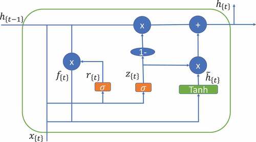
Figure 1 shows a diagram of a GRU unit. The activation function is usually tanh or a sigmoid function. The GRU was developed as a solution for short-term memory. It has built-in mechanisms called gates that regulate the flow of information (C. Li et al., 2018; Zhang et al., 2021).

Figure 1. The cell structure of a Gated Recurrent Unit. (Mateus et al., 2021).

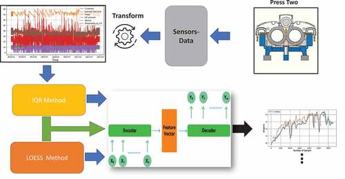
Figure 2 shows the scheme of the proposed method, with the function of extracting the data treatment by means of the two proposed methods, in order to have a predictive model with good predictive capacity. It is possible to predict patterns of failures in the variables of the presses.

Figure 2. Diagram showing the flow the process data, from the press’ sensors to predictions.

2.2. Model evaluation

The Mean Absolute Percentage Error (MAPE) was used as a model performance measure. It is calculated according to Equation 5(5) $MAPE=\frac{1}{n}\sum _{t=1}^n\frac{|Y_t-{\hat{Y}}_t|}{|Y_t|}$(5) . It is a metric commonly used to estimate AI models’ error and works best when there are no extremes in the data, namely, zeros cannot exist in the actual output, so that the value of the fraction can be calculated.

(5) $MAPE=\frac{1}{n}\sum _{t=1}^n\frac{|Y_t-{\hat{Y}}_t|}{|Y_t|}$(5)

Where:

• $n$ is total number of observations;

• $Y_t$ is the actual value;

• ${\hat{Y}}_t$ is the value predicted by the model.

Root Mean Square Error (RMSE) was also used to validate the results, which is given by the mathematical formula:

(6) $RMSE=\sqrt{\frac{1}{n}\sum _{t=1}^n{(Y_t-{\hat{Y}}_t)}^2}$(6)

The Mean Average Error (MAE), which evaluates the magnitude of the average error in a set of predictions without considering their direction, has also been used.

(7) $MAE=\frac{1}{n}\sum _{t=1}^n|Y_t-{\hat{Y}}_t|$(7)

3. Data pre-processing

In order to ensure quality of data fed to the machine learning models, one of the first steps of the present study was the analysis and elimination of discrepant data which could interfere with the convergence of the learning algorithms. Two methods were used: the first was the Elimination of lower and upper extreme values, the second was based on smoothing using linear regression.

3.1. Eliminating discrepant data

The method of eliminating discrepant values is based on the idea that extreme values are most probably data reading failures. They often happen due to sensor failures, communication interference or other type of problems during data acquisition. As a result, the dataset sometimes contains invalid samples such as readings outside of the expected sensor ranges, or zero when the machine was stopped. Those samples can be eliminated, so that they do not negatively affect the machine learning process.

In the present work, limits were calculated for each variable and the samples out of the allowed range were replaced by the average. The limits were calculated using the following equations:

(8) $Q_{\frac{1}{4}}=\frac{1}{4}(n+1)$(8)

(9) $Q_{\frac{3}{4}}=\frac{3}{4}(n+1)$(9)

(10) $IQR=Q_{\frac{1}{4}}-Q_{\frac{3}{4}}$(10)

(11) $Dow{n}_{limit}=Q_{\frac{1}{4}}-K\times IQR$(11)

(12) $U{p}_{limit}=Q_{\frac{3}{4}}+K\times IQR$(12)

$Dow{n}_{limit}$ is the lower limit accepted for the variable, calculated by subtracting the constant $k$ multiplied by $IQR$ to $Q_{\frac{1}{4}}$. $U{p}_{limit}$ is the upper limit accepted for the variable, calculated by adding the constant $k$ multiplied by $IQR$ to $Q_{\frac{3}{4}}$, where $k$ is the constant of variation of the limits. The limits are calculated for each variable. Sample data points that contain values that are out of the interval $[Dow{n}_{limit},U{p}_{limit}]$ are replaced by the average.

3.2. Data smoothing

LOWESS/LOESS (locally weighted/estimated scatterplot smoothing) is a non-parametric regression technique developed by Cleveland (Cleveland, 1981). Robust locally weighted regression is a method for smoothing variables, $(x_i,y_i),i=1,\cdots ,n$, in which the fitted value at $z_k$ is the value of a polynomial fit to the data using weighted least squares, where the weight for $(x_i,y_i)$ is large if $x_i$ is close to $x_k$ and small if it is not. The number of samples ($n$) used for each local approximation ($z_k$) is a parameter of the model. The degree of the polynomial function is also a parameter of the model. Often the polynomial degree is 1, which means a linear regression is performed.

Recent research has used the LOWESS smoothing technique in order to optimize the process of training and testing deep neural networks (Bury et al., 2021; Kulkarni et al., 2021). According to Phyo et al. (2019), LOWESS/LOESS procedure is used to overcome the problem of discrepant values. The study by (Jeenanunta et al., 2019) presents the influence that the LOWESS smoothing processing method has on the forecast errors of time series. According to Dai et al. (2022) all five different smoothing methods used in the study can improve the prediction performance of the GRU model. Among them, LOWESS smoothing can produce the smallest prediction error.

3.3. Data before and after pre-processing

The data set used in the present research contains samples from two paper pulp presses. The samples were collected through several sensors that are installed in the two presses, in a large industrial plant. The sensors read the following variables: i) Current Intensity: current absorbed by the press motor, in Ampere; ii) Hydraulic Unit Oil Level (in percentage); iii) Torque of the motor (in N.m); iv) VAT Pressure: Pressure inside the Cuba (in KPa); v) Rotation Velocity: velocity of rotation of the press’ rolls, in rotations per minute; vi) Temperature at Hydraulic Unit, in degree Celsius. There are nominal values for each of those variables, from the press manufacturer. Deviations from the expected intervals, which are related among them, may cause equipment failure.

A plot of the original data is shown in Figure 3. The samples were registered with sampling period of 1 min for press number 2 and 5 min for press number 4. For most many of the experiments the dataset was downsampled, in order to reduce processing time. The downsampling rate varied, although most of the time the 12 or 60 samples of each hour are averaged, which is equivalent to using a sampling period of 1 hour.

Figure 3. Plot of the variables for press number 4, before any data pre-processing. The variables contain a large amount of noise.

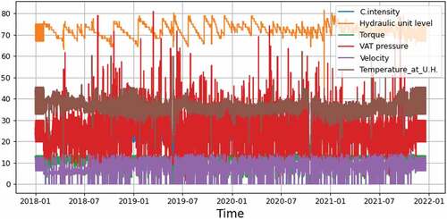
The original data contain many discrepant samples, shown as extremes values in Figure 3. There are spikes and sudden variations, which are mostly noise for the machine learning algorithms. Using the methods described in the previous subsections, most of the extremes are removed, specially the zeroes which were abundant and may be caused by reading errors or production line stops.

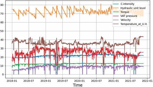
The discrepant data cleaning eliminates many extreme values. Nonetheless, the amplitude and frequency of variations still make the readings very unstable. Testing the LOWESS method with a window size of 3 days it is possible to verify that in Figure 4 there is a significant reduction of the extreme values which were present in Figure 3, without affecting the trends that the data was showing. The trends are maintained and the variables are smoothed.

Figure 4. Plot of the variables for press number 4, after data pre-processing. The variables contain a low amount of noise.

4. Case study

4.1. Analysis of correlations before and after pre-processing

In order to have a better understanding on the impact of filtering the data using the LOWESS filter, an analysis of variable autocorrelation was performed. Figure 5 shows autocorrelations of the six variables before cleaning and applying the LOWESS filter. As the charts show, the correlations decay at a fast pace. The current intensity and torque, which are two very important variables, show autocorrelations of almost zero at 400 lags, which corresponds to 17 days. As for the variables VAT pressure, Hydraulic unit oil level, and Temperature, the correlation reaches almost zero at 500 lags, corresponding to 21 days. For velocity the decay happens at a slower pace, where the correlation is still about 0.1 at 1000 lags, corresponding to 42 days.

Figure 5. Variable autocorrelations, before cleaning and filtering the data.

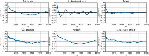
This shows that prediction with 30 days in advance is an ambitious goal, although not impossible, specially combining all variables into a multivariate model as done before (Mateus et al., 2021).

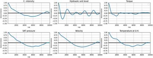
Figure 6 shows the autocorrelations of the variables after data cleaning and filtering using the LOWESS method with 36 days window size. As the figure shows, the correlations for all variables have become larger than shown in Figure 5. The hydraulic unit oil level is the one with faster autocorrelation decay. The other variables show a good improvement, indicating better chances of small prediction errors.

Figure 6. Autocorrelation for the all variables, obtained after cleaning and smoothing the data using LOWESS with 36 days window.

4.2. Prediction and comparison of the results

For model validation the data were divided into two subsets. The training subset uses the first 80% of the total data and the test subset contains the remainder 20% of the data samples.

The purpose of the experiments is to find the best data preprocessing methods, neural model architectures and hyperparameters that produce the best results predicting future behaviour of the paper pulp presses. The tests were performed using a GRU neural network with data encoder and decoder architecture, for it was the architecture that showed best results in previous work (Mateus et al., 2021).

Compared to LSTM models, GRU models have fewer parameters and simpler structures. (Gao et al., 2020) show that GRU models perform as well as LSTM models. (Mateus et al., 2021) show that GRU has a higher capacity in terms of the sampling rate.

The experiments aim at testing different pre-processing methods. Elimination of discrepant values is Method 1. Data smoothing using the LOWESS filter is Method 2. The combination of both – first the elimination of discrepant data, then smoothing –, is called Method (1, 2). The architecture of the neural network was the same for all the experiments, and it is the same that showed best results in previous work. Nonetheless, experiments were still performed with a smaller and faster GRU, with just 50 units, and a larger and slower network, with 500 units.

For press number 2, LOWESS method presented better results using a window of 5 days. The window size was halved because the number of data samples available from press 2 was too small for using larger windows. The dataset for press 4 contains 34,800 hours of data, while the dataset for press 2 contains just 24,096 hours of data.

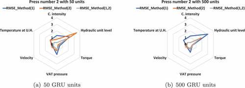
Figure 7 shows the RMSE values of predictions for press 2, with the smaller and the larger GRU neural networks, with and without LOWESS filtering. As the figure shows, the prediction errors are much smaller when data are filtered. The difference is even more notorious in the larger network. For the same press and the same architecture, increasing the GRU units of the neural network to 500, it is verified that the combination of the methods leads to the same result, but with much smaller errors. The hydraulic variable in particular shows a larger error for both network structures.

Figure 7. RMSE of the best models for press 2, using the two different methods for pre-processing data, for the smaller and larger GRU networks. Method 1 only removes discrepant data. Method 2 smoothes the data using a LOWESS filter. Method (1,2) is the application of both. (a) prediction test with 50 GRU units with the two data processing methods, (b) prediction test with 500 GRU units with the two data processing methods.

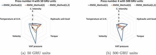
For data originary from press number 4, the LOWESS filter presented better results using a window of 36 days. From the RMSE diagram in Figure 8, it can be seen that the results for press 4 also show much lower errors when the LOWESS filter is applied. The smaller model, with 50 GRU neural units, shows errors slightly larger than the larger model. For the same press using 500 GRU neural units, the RMSE errors are smaller, as demonstrated by the smaller area of the chart polygons.

Figure 8. RMSE for predictions of press 4 using the different data pre-processing methods. LOWESS filtering and 500 GRU units result in smaller RMSE errors. (a) prediction test with 50 GRU units with the two data processing methods, (b) prediction test with 500 GRU units with the two data processing methods.

Applying the two methods to press 2 data, it can be seen that while the errors in Table 3 are small, the important information are omitted from the graph in Figure 9, which is not good for possible press failure analysis.

Figure 9. Signals and forecast results for press 2, with 30 day advance, using the two data processing methods, both removal of discrepant data and data smoothing using LOWESS filtering with 36 days window. The blue lines represent the actual value. The Orange and green lines are predictions, respectively, in the train and test subsets.

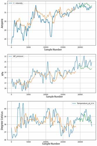
Table 3. Prediction error results for 30 days advance forecast, using the two data preprocessing methods, removal of discrepant data and smoothing (LOWESS 36 days), for the 500 unit GRU with 5 days window, for press 2.

			Prediction errors for press 2
	C. Intensity	Hydraulic	Torque	VAT	Velocity	Temperature
MAPE	0.62	1.85	2.24	3.91	10.27	0.96
MAE	0.2	1.39	0.35	0.82	0.57	0.38
RMSE	0.23	1.55	0.37	0.95	0.6	0.5

Figure 10 shows the result of predicting the model with the better method of data processing for the press 4, which in this case falls on the intersection of the two methods. From the Table 4 it can be seen that the error is smaller.

Figure 10. Signals and forecast results for press 4, with 30 day advance, using the two data processing methods, both removal of discrepant data and data smoothing using LOWESS filtering with 36 days window. The blue lines represent the actual value. The Orange and green lines are predictions, respectively, in the train and test subsets.

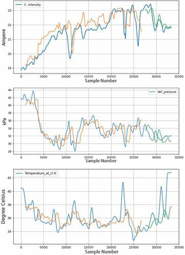
Table 4. Prediction error results for 30 days advance forecast, using the two data preprocessing methods, removal of discrepant data and smoothing (LOWESS 36 days), for the 500 unit GRU with 5 days window, for press 4.

			Prediction errors for press 4
	C. Intensity	Hydraulic	Torque	VAT	Velocity	Temperature
MAPE	1.2	1.12	2.32	1.6	2.77	1.36
MAE	0.27	0.8	0.18	0.51	0.26	0.5
RMSE	0.30	1.00	0.20	0.61	0.30	0.69

5. Discussion

Data processing removing discrepant data simplifies the learning process of the RNN model and also leads to an improvement in the prediction results. The results obtained showed an improvement with data from both presses when discrepant data samples were replaced by the average. An analysis of autocorrelations shows that the use of data processing methods results in higher correlations for larger periods of time, when compared to untreated data as shown in Figure 9, and Figure 10.

In the literature review, no other studies were found to deal with forecast for industrial paper pulp presses using encoder-decoder architectures and recurrent neural units. The present work and comparative analysis of the results obtained for two industrial presses show that the architecture proposed is versatile and the same network architecture can be applied to both datasets, forecasting with acceptable errors after training. The larger architecture, using 500 GRU units, is slower and produces lower errors. The smaller architecture, with just 50 units, is faster and is still able to learn, although produces larger errors. Using data smoothed with the LOWESS filter, the learning process is highly facilitated. The prediction errors obtained in a 30 days advance forecas are smaller, with MAPE in general less than 10 %.

Compared to previous results (Mateus et al., 2021), the MAPE for the Current Intensity for press 2 decreased from 2.30% to 0.62%. For the Hydraulic oil level the MAPE decreased from 2.8% to 1.85%. For the Torque, the MAPE decreased from 2.85% to 2.24%. For the VAT pressure, the MAPE comes from 9.87% to 3.91%. For the Velocity, MAPE decreased from 11.8% to 10.27%. Finally, for the Temperature the MAPE decreased from 2.66% to 0.96%.

The quality of the results is confirmed visually in the charts, where the charts are in general easy to read and show the main trends of the variables.

In summary, we demonstrate that the approach done innovates, namely the following one: -The conjugation of Elimination of lower and upper discrepant values and LOWESS to data processing before inserting them in the NN, what proved to have better results than the other approaches described in the literature.

Additionally, the approach proposed can be adapted to other types of equipment, helping to solve prediction problems and contributing to increasing their availability.

6. Conclusions

In modern industries, prediction algorithms can anticipate future trends and contribute for better management decisions, namely in predictive maintenance. The results obtained in the present work demonstrate the applicability of recurrent neural networks (i.e. GRUs) in predicting future behavior in the paper press industry. The encoder and decoder architecture with GRU unit showed good results learning data from two different industrial pulp presses, and by applying the LOWESS technique the prediction errors decrease considerably, as described in Section 5.

Data pre-processing can play a very important role in improving the predictions. In the present work, filtering out discrepant data and smoothing using a LOWESS filter reduced the MAPE errors for all variables.

The results show that it is possible to forecast future behavior of industrial paper pulp presses up to 30 days in advance with good degree of certainty. That can be a good opportunity for optimizing maintenance decisions, reducing downtime and costs.

As limitations of the present approach, it must be referred that the method requires near real time operation, demanding high-speed networks and high power computation for monitoring the equipment and producing forecasts in advance. Additionally, the approach being based on machine learning algorithms produces only estimates with a degree of uncertainty.

In future work, other variables can be included in the study, namely through the inclusion of stock market variables in the model. These variables will aim to improve the predictive model, exploring the link between the stock market and the need for the production of the machines and their corresponding availability.

Abbreviations

Table

AI	Artificial Intelligence
ANN	Artificial Neural Networks
IoT	Internet of Things
IQR	Interquartile Range
NN	Neural Networks
GRU	Gated Recurrent Units
LSTM	Long Short-Term Memory
MAE	Mean Absolute Error
MAPE	Mean Absolute Percentage Error
RMSE	Root Mean Square Error
RNN	Recurrent Neural Networks
AF	Activation Function

Acknowledgments

The research leading to these results has received funding from the European Union’s Horizon 2020 research and innovation programme under the Marie Sklodowvska-Curie grant agreement 871284 project SSHARE and the European Regional Development Fund (ERDF) through the Operational Programme for Competitiveness and Internationalization (COMPETE 2020), under Project POCI-01-0145-FEDER-029494, and by National Funds through the FCT—Portuguese Foundation for Science and Technology, under Projects PTDC/EEI-EEE/29494/2017, UIDB/04131/2020, and UIDP/04131/2020.

Disclosure statement

The authors declare that do not have any conflict of interest.

References

- Abbasi, T., Lim, K. H., & Yam, K. S. (2019). Predictive maintenance of oil and gas equipment using recurrent neural network. IOP Conference Series: Materials Science and Engineering, 495:12067.
- Almeida Pais, J. E. D., Raposo, H. D. N., Farinha, J. T., Cardoso, A. J. M., & Marques, P. A. (2021). Optimizing the life cycle of physical assets through an integrated life cycle assessment method. Energies, 14(19), 6128. https://doi.org/10.3390/en14196128
- Asgarpour, M., Sørensen, J., Vazquez, S. L., Kulkarni, C. S., Strom, T. H., Hill, B. L., Smalling, K. M., & Quach, C. C. (2018). Bayesian based prognostic model for predictive maintenance of offshore wind farms. International Journal of Prognostics and Health Management, 9(1). https://doi.org/10.36001/ijphm.2018.v9i1.2700
- Balevi, E., Rabee, F. T. A., & Gitlin, R. D. (2018). Aloha-noma for massive machine-to-machine iot communication. In 2018 IEEE International Conference on Communications (ICC), 1–22.
- Bury, T. M., Sujith, R., Pavithran, I., Scheffer, M., Lenton, T. M., Anand, M., & Bauch, C. T. (2021). Deep learning for early warning signals of tipping points. Proceedings of the National Academy of Sciences, 118(39):e2106140118.
- Canizo, M., Onieva, E., Conde, A., Charramendieta, S., & Trujillo, S. (2017). Real-time predictive maintenance for wind turbines using big data frameworks. 2017 IEEE International Conference on Prognostics and Health Management, ICPHM 2017, 70–77.
- Choi, Y., Kwun, H., Kim, D., Lee, E., & Bae, H. (2020). Method of predictive maintenance for induction furnace based on neural network. 2020 IEEE International Conference on Big Data and Smart Computing (BigComp), 609–612.
- Chong, M. M., Abraham, A., & Paprzycki, M. (2004). Traffic accident analysis using decision trees and neural networks. International Journal of Information Technology and Computer Science, 6, 22–28. https://doi.org/10.48550/arXiv.cs/0405050
- Cho, K., van Merrienboer, B., Bahdanau, D., & Bengio, Y. 2014. On the properties of neural machine translation: Encoder-decoder approaches. CoRR, 1409, abs, 1259. https://doi.org/10.48550/arXiv.1409.1259
- Chui, K. T., Gupta, B. B., & Vasant, P. (2021). A genetic algorithm optimized rnn-lstm model for remaining useful life prediction of turbofan engine. Electronics, 10(3), 285. https://doi.org/10.3390/electronics10030285
- Cleveland, W. S. (1981). Lowess: A program for smoothing scatterplots by robust locally weighted regression. The American Statistician, 35(1), 54. https://doi.org/10.2307/2683591
- Cline, B., Niculescu, R. S., Huffman, D., & Deckel, B. (2017). Predictive maintenance applications for machine learning. Proceedings - Annual Reliability and Maintainability Symposium.
- Couso, I., Borgelt, C., Hullermeier, E., & Kruse, R. (2019). Fuzzy sets in data analysis: From statistical foundations to machine learning. IEEE Computational Intelligence Magazine, 14(1), 31–44. https://doi.org/10.1109/MCI.2018.2881642
- Cross, M. (1988). Raising the value of maintenance in the corporate environment. Management Research News, 11(3), 8–11. https://doi.org/10.1108/eb027976
- Dai, Y., Wang, Y., Leng, M., Yang, X., & Zhou, Q. (2022). Lowess smoothing and random forest based gru model: A short-term photovoltaic power generation forecasting method. Energy, 256, 124661. https://doi.org/10.1016/j.energy.2022.124661
- Dalzochio, J., Kunst, R., Pignaton, E., Binotto, A., Sanyal, S., Favilla, J., & Barbosa, J. (2020). Machine learning and reasoning for predictive maintenance in industry 4.0: Current status and challenges. Computers in Industry, 123, 103298. https://doi.org/10.1016/j.compind.2020.103298
- Drath, R., & Horch, A. (2014). Industrie 4.0: Hit or hype? [industry forum]. IEEE Industrial Electronics Magazine, 8(2), 56–58. https://doi.org/10.1109/MIE.2014.2312079
- Edwards, D. J., Holt, G. D., & Harris, F. (1998). Predictive maintenance techniques and their relevance to construction plant. Journal of Quality in Maintenance Engineering, 4(1), 25–37. https://doi.org/10.1108/13552519810369057
- Eklund, P. (1998). of Intelligent Information Systems. v9 i1, A. H., and undefined 2002. A performance survey of public domain supervised machine learning algorithms. https://www.researchgate.net/profile/Peter-Eklund/publication/2767745_A_Performance_Survey_of_Public_Domain_Supervised_Machine_Learning_Algorithms/links/0fcfd50b315bee877a000000/A-Performance-Survey-of-Public-Domain-Supervised-Machine-Learning-Algorithms.pdf
- Erboz, G. (2017). How to define industry 4.0: Main pillars of industry 4.0. Managerial Trends in the Development of Enterprises in Globalization Era, 761, 767. https://www.researchgate.net/profile/Gizem-Erboz-2/publication/326557388_How_To_Define_Industry_40_Main_Pillars_Of_Industry_40/links/5fc553374585152e9be7f201/How-To-Define-Industry-40-Main-Pillars-Of-Industry-40.pdf
- Florea, G., Paraschiv, A., & Cimpoesu, E. (2012). Wind farm noise monitoring used for predictive maintenance. IFAC Proceedings Volumes, 45:1822–1827.
- Gao, S., Huang, Y., Zhang, S., Han, J., Wang, G., Zhang, M., & Lin, Q. (2020). Short-term runoff prediction with gru and lstm networks without requiring time step optimization during sample generation. Journal of Hydrology, 589, 125188. https://doi.org/10.1016/j.jhydrol.2020.125188
- Glistau, E., & Coello Machado, N. I. (2018). Industry 4.0, logistics 4.0 and materials - chances and solutions. Materials Science Forum, 919, 307–314. https://doi.org/10.4028/www.scientific.net/MSF.919.307
- Gorski, E. G., de Freitas Rocha Loures, E., Santos, E. A. P., Kondo, R. E., & Martins, G. R. D. N. (2021). Towards a smart workflow in cmms/eam systems: An approach based on ml and mcdm. Journal of Industrial Information Integration, 100278. https://doi.org/10.1016/j.jii.2021.100278
- He, K., Liu, Z., Sun, Y., Mao, L., & Lu, S. (2022). Degradation prediction of proton exchange membrane fuel cell using auto-encoder based health indicator and long short-term memory network. International Journal of Hydrogen Energy, 47, 35055–35067. https://doi.org/10.1016/j.ijhydene.2022.08.092
- Huang, Y., & Li, G. (2010). Descriptive models for internet of things. In 2010 International Conference on Intelligent Control and Information Processing, 483–486.
- Husain, S., Prasad, A., Kunz, A., Papageorgiou, A., & Song, J. (2014). Recent trends in standards related to the internet of things and machine-to-machine communications. Journal of Information and Communication Convergence Engineering, 12(4), 228–236. https://doi.org/10.6109/jicce.2014.12.4.228
- Jabeur, S. B., Gharib, C., Mefteh-Wali, S., & Arfi, W. B. (2021). Catboost model and artificial intelligence techniques for corporate failure prediction. Technological Forecasting and Social Change, 166, 120658. https://doi.org/10.1016/j.techfore.2021.120658
- Jeenanunta, C., Abeyrathna, K. D., Dilhani, M. H. M. R. S., Hnin, S. W., & Phyo, P. P. (2019). Time series outlier detection for short-term electricity load demand forecasting. International Scientific Journal of Engineering and Technology (ISJET), 2(1), 37–50. https://ph02.tci-thaijo.org/index.php/isjet/article/view/175908
- Jezzini, A., Ayache, M., Elkhansa, L., Makki, B., & Zein, M. (2013). Effects of predictive maintenance(pdm), proactive maintenace(pom) & preventive maintenance(pm) on minimizing the faults in medical instruments. In 2013 2nd International Conference on Advances in Biomedical Engineering, 53–56.
- Ji, W., & Wang, L. (2017). Big data analytics based fault prediction for shop floor scheduling. Journal of Manufacturing Systems, 43, 187–194. https://doi.org/10.1016/j.jmsy.2017.03.008
- Kalsoom, T., Ramzan, N., Ahmed, S., & Ur-Rehman, M. (2020). Advances in sensor technologies in the era of smart factory and industry 4.0. Sensors, 20(23), 6783. https://doi.org/10.3390/s20236783
- Kim, D. Y., Jeong, Y. S., & Kim, S. 2017. Data-filtering system to avoid total data distortion in iot networking. Symmetry, 9(16), 16. 2017. https://doi.org/10.3390/sym9010016.
- Koprinkova-Hristova, P. D., Hadjiski, M. B., Doukovska, L. A., & Beloreshki, S. V. (2011). Recurrent neural networks for predictive maintenance of mill fan systems. International Journal of Electronics and Telecommunications, 57(3), 401–406. https://doi.org/10.2478/v10177-011-0055-2
- Kulkarni, H., Thangam, M., & Amin, A. P. (2021). Artificial neural network-based prediction of prolonged length of stay and need for post-acute care in acute coronary syndrome patients undergoing percutaneous coronary intervention. European Journal of Clinical Investigation, 51(3), e13406. https://doi.org/10.1111/eci.13406
- Lee, J., Ni, J., Djurdjanovic, D., Qiu, H., & Liao, H. 2006. Intelligent prognostics tools and e-maintenance. Computers in Industry, 57(6), 476–489. E-maintenance Special Issue. https://doi.org/10.1016/j.compind.2006.02.014
- Lei, X., Sandborn, P., Bakhshi, R., Kashani-Pour, A., & Goudarzi, N. (2015). Phm based predictive maintenance optimization for offshore wind farms. In 2015 IEEE Conference on Prognostics and Health Management (PHM), 1–8.
- L’Heureux, A., Grolinger, K., Elyamany, H. F., & Capretz, M. A. (2017). Machine learning with big data: Challenges and approaches. IEEE Access, 5, 7776–7797. https://doi.org/10.1109/ACCESS.2017.2696365
- Lim, T. S., Loh, W. Y., & Shih, Y. S. 2000. A comparison of prediction accuracy, complexity, and training time of thirty-three old and new classification algorithms. Machine Learning, 40(3), 203–228. 2000. https://doi.org/10.1023/A:1007608224229
- Li, H., Parikh, D., He, Q., Qian, B., Li, Z., Fang, D., & Hampapur, A. (2014). Improving rail network velocity: A machine learning approach to predictive maintenance.Transportation Research Part C: Emerging Technologies, 45, 17–26. Advances in Computing and Communications and their Impact on Transportation Science and Technologies. https://doi.org/10.1016/j.trc.2014.04.013
- Liu, R., Yang, B., Zio, E., & Chen, X. (2018). Artificial intelligence for fault diagnosis of rotating machinery: A review. Mechanical Systems and Signal Processing, 108, 33–47. https://doi.org/10.1016/j.ymssp.2018.02.016
- Li, C., Xie, C., Zhang, B., Chen, C., & Han, J. (2018). Deep fisher discriminant learning for mobile hand gesture recognition. Pattern Recognition, 77, 276–288. https://doi.org/10.1016/j.patcog.2017.12.023
- Lv, Y., Zhou, Q., Li, Y., & Li, W. (2021). A predictive maintenance system for multi-granularity faults based on adabelief-bp neural network and fuzzy decision making. Advanced Engineering Informatics, 49, 101318. https://doi.org/10.1016/j.aei.2021.101318
- Lykourentzou, I., Giannoukos, I., Nikolopoulos, V., Mpardis, G., & Loumos, V. (2009). Dropout prediction in e-learning courses through the combination of machine learning techniques. Computers & Education, 53(3), 950–965. https://doi.org/10.1016/j.compedu.2009.05.010
- Markiewicz, M., Wielgosz, M., Bochenski, M., Tabaczynski, W., Konieczny, T., & Kowalczyk, L. (2019). Predictive maintenance of induction motors using ultra-low power wireless sensors and compressed recurrent neural networks. IEEE Access, 7, 178891–178902. https://doi.org/10.1109/ACCESS.2019.2953019
- Martins, A. B., Farinha, J. T., & Cardoso, A. M. (2020). Calibration and certification of industrial sensors – A global review. WSEAS Transactions on Systems and Control, 15, 394–416. https://doi.org/10.37394/23203.2020.15.41
- Martins, A., Fonseca, I., Farinha, J. T., Reis, J., & Cardoso, A. M. 2021. Maintenance prediction through sensing using hidden Markov models—a case study. Applied Sciences, 11(7685), 7685. 2021. https://doi.org/10.3390/app11167685
- Mateus, B. C., Mendes, M., Farinha, J. T., Assis, R., & Cardoso, A. M. (2021). Comparing lstm and gru models to predict the condition of a pulp paper press. Energies, 14(21), 6958. https://doi.org/10.3390/en14216958
- Miller, K., Hettinger, C., Humpherys, J., Jarvis, T., & Kartchner, D. (2017). Forward thinking: Building deep random forests.
- Narendra, N., Ponnalagu, K., Ghose, A., & Tamilselvam, S. (2015). Goal-driven context-aware data filtering in iot-based systems. 2015 IEEE 18th International Conference on Intelligent Transportation Systems, 2172–2179.
- Nascimento, R. G., & Viana, F. A. (2019). Fleet prognosis with physics-informed recurrent neural networks. Structural Health Monitoring 2019: Enabling Intelligent Life-Cycle Health Management for Industry Internet of Things (IIOT) - Proceedings of the 12th International Workshop on Structural Health Monitoring, 2:1740–1747.
- Phyo, P. P., Jeenanunta, C., & Hashimoto, K. (2019). Electricity load forecasting in Thailand using deep learning models. International Journal of Electrical and Electronic Engineering & Telecommunications, 8(4), 221–225. https://doi.org/10.18178/ijeetc.8.4.221-225
- Qiu, J., Wu, Q., Ding, G., Xu, Y., & Feng, S. (2016). A survey of machine learning for big data processing. Eurasip Journal on Advances in Signal Processing, 2016, 1–16. https://doi.org/10.1186/s13634-016-0355-x
- Rivas, A., Fraile, J. M., Chamoso, P., González-Briones, A., Sittón, I., & Corchado, J. M. (2019). A predictive maintenance model using recurrent neural networks. Advances in Intelligent Systems and Computing, 950, 261–270. https://doi.org/10.1007/978-3-030-20055-8_25
- Rodrigues, J. A., Farinha, J. T., Mendes, M., Mateus, R., & Cardoso, A. (2021). Short and long forecast to implement predictive maintenance in a pulp industry. Eksploatacja I Niezawodnosc - Maintenance and Reliability, 24(1), 33–41. https://doi.org/10.17531/ein.2022.1.5
- Santra, A. S., & Lin, J.-L. 2019,January. Integrating long short-term memory and genetic algorithm for short-term load forecasting. Energies 12:11 2040. Number: 11 Publisher: Multidisciplinary Digital Publishing Institute https://doi.org/10.3390/en12112040
- Schwenk, H., & Bengio, Y. (2000). Boosting neural networks. Neural Computation, 12(8), 1869–1887. https://doi.org/10.1162/089976600300015178
- Sherif, Y. S., & Smith, M. L. (1981). Optimal maintenance models for systems subject to failure–a review. Naval Research Logistics Quarterly, 28, 47–74. https://doi.org/10.1002/nav.3800280104
- Spendla, L., Kebisek, M., Tanuska, P., & Hrcka, L. (2017). Concept of predictive maintenance of production systems in accordance with industry 4.0. In 2017 IEEE 15th International Symposium on Applied Machine Intelligence and Informatics (SAMI), 000405–000410.
- Tipping, M. E. (2003). Bayesian inference: An introduction to principles and practice in machine learning. Lecture Notes in Computer Science (Including Subseries Lecture Notes in Artificial Intelligence and Lecture Notes in Bioinformatics), 3176, 41–62. https://doi.org/10.1007/978-3-540-28650-9_3
- Tsibulnikova, M. R., Pham, V. A., Aikina, T. Y., Xue-feng, L., Xiao-ben, L., Jan-ding, H., Al, Abbasi, T., Lim, K. H., & Yam, K. S. (2019). Predictive maintenance of oil and gas equipment using recurrent neural network. IOP Conference Series: Materials Science and Engineering, 495:12067.
- Turnbull, A., & Carroll, J. (2021). Cost benefit of implementing advanced monitoring and predictive maintenance strategies for offshore wind farms. Energies, 14(16), 4922. https://doi.org/10.3390/en14164922
- Udo, W., & Muhammad, Y. (2021). Data-driven predictive maintenance of wind turbine based on scada data. IEEE Access, 9, 162370–162388. https://doi.org/10.1109/ACCESS.2021.3132684
- Wang, S.-C. (2003). Artificial neural network. Interdisciplinary Computing in Java Programming, 81–100. https://doi.org/10.1007/978-1-4615-0377-4_5
- Wang, F.-K., Amogne, Z. E., Chou, J.-H., & Tseng, C. (2022). Online remaining useful life prediction of lithium-ion batteries using bidirectional long short-term memory with attention mechanism. Energy, 254, 124344. https://doi.org/10.1016/j.energy.2022.124344
- Wang, Q., Bu, S., & He, Z. (2020). Achieving predictive and proactive maintenance for high-speed railway power equipment with lstm-rnn. IEEE Transactions on Industrial Informatics, 16(10), 6509–6517. https://doi.org/10.1109/TII.2020.2966033
- Wu, H., Huang, A., & Sutherland, J. W. (2020). Avoiding environmental consequences of equipment failure via an lstm-based model for predictive maintenance. Procedia Manufacturing, 43:666–673. Sustainable Manufacturing - Hand in Hand to Sustainability on Globe: Proceedings of the 17th Global Conference on Sustainable Manufacturing.
- Yam, R. C., Tse, P. W., Li, L., & Tu, P. 2001. Intelligent predictive decision support system for condition-based maintenance. The International Journal of Advanced Manufacturing Technology, 17(5), 383–391. 2001. https://doi.org/10.1007/s001700170173
- Zfle, M., Moog, F., Lesch, V., Krupitzer, C., & Kounev, S. (2021). A machine learning-based workflow for automatic detection of anomalies in machine tools. ISA Transactions, 121, 180–190. https://doi.org/10.1016/j.isatra.2021.03.036
- Zhang, J., Zeng, Y., & Starly, B. (2021). Recurrent neural networks with long term temporal dependencies in machine tool wear diagnosis and prognosis. SN Applied Sciences, 3(4), 1–13. https://doi.org/10.1007/s42452-021-04427-5
- Zhikun, H., Bin, J., Linzi, Y., & Xiaolong, C. (2013). Predictive maintenance strategy of variable period of power transformer based on reliability and cost. 2013 25th Chinese Control and Decision Conference, CCDC 2013, 4803–4807.
- Zhou, C., Liu, X., Chen, W., Xu, F., & Cao, B. (2018). Optimal sliding mode control for an active suspension system based on a genetic algorithm. Algorithms, 11(12), 205. https://doi.org/10.3390/a11120205
- Zhou, L., Pan, S., Wang, J., & Vasilakos, A. V. (2017). Machine learning on big data: Opportunities and challenges. Neurocomputing, 237, 350–361. https://doi.org/10.1016/j.neucom.2017.01.026
- Zibar, D., Piels, M., Jones, R., & Schäeffer, C. G. (2016). Machine learning techniques in optical communication. Journal of Lightwave Technology, 34(6), 1442–1452. https://doi.org/10.1109/JLT.2015.2508502