Operating minimally intelligent agent-based manufacturing systems across the Average demand Interval – coefficient of variation (ADI-CV) demand state space

ABSTRACT

Minimally Intelligent Agent-Based Manufacturing concerns the provision of agents with the minimal intelligence required to autonomously negotiate and broker work across machines and jobs. The minimal intelligence of agents can be updated in real-time and when coupled with technologies, such as Additive Manufacturing (AM), robotics, automated inventory, and Computer Numerical Control (CNC) affords highly flexible, re-configurable, resilient and responsive systems. The concept has become topical as changes to global supply chains are necessitating a shift to responsive and resilient on-demand manufacturing. However, understanding and characterising how these systems operate under various demand profiles is required to support operators operating these future systems. This paper reports a numerical study into the operating behaviour of minimally intelligent agent-based manufacturing systems operating across the Average Demand Interval and Coefficient of Variation (ADI-CV) demand state space. An established state space used in spare part supply chain research. The results show minimally intelligent manufacturing systems are stable across much of the ADI-CV demand space 85%, 63% and 76–84% for constant, triangular and lognormal manufacturing time distribution profiles respectively. The stability is largely independent of the combination of intelligence. Rather, the combination of intelligence impacts job Time-in-System and system response.

KEYWORDS:

• Minimal intelligence
• artificial intelligence
• agent-based modelling
• Spare-parts-on-demand (SPOD)
• Average demand interval - coefficient of variation (ADI-CV)

1. Introduction

Global manufacturing supply chains are experiencing unprecedented change (Luman & Fechner, 2022). Societal behaviours, such as the ‘Maker’ movement, mass-customisation, and the desire for rapid delivery are requiring an on-demand and responsive manufacturing capability (Doussard et al., 2018; Hamalainen & Karjalainen, 2017). Net Zero and Circular Economy agendas are demanding change in how society manufactures and supplies itself with organisations wishing to move away from stocking components/products (Forum, 2021). Servitisation and the right-to-repair movement is requiring extended life products that can be maintained, repaired and overhauled (Ozturkcan, 2023). This, in turn, has increased the demand for spare part production. Market fragility and supply chain uncertainty is increasing the risk in forecasting supply and demand. This is resulting in smaller and more intermittent orders with small turnaround times. National Security policies are also encouraging the re-shoring of manufacturing (Gur & Dilek, 2023). And an increase in global ‘shock’ events, such as COVID-19 and the war in Ukraine, is requiring further resilience in supply chains (Remko, 2020).

These events have inflated the market tail resulting in a Big Demand (variety, volume, velocity, veracity, and value) of items that need to be globally-locally produced. Rather than steady and predictable demand profiles, demand for items in the tail are more intermittent, lumpy and/or erratic in nature.

The spare parts industry has observed this type of demand for many years and has employed numerous forecasting strategies to overcome them (Boylan & Syntetos, 2009; J. Gopsill et al., 2022; Pinçe et al., 2021). However, many rely on holding stock, which is both economically and sustainably challenging. Value is ‘locked’ into stored items (increasing and decreasing with market trends) and energy and resource is used to produce and store items that may never be used. The ideal scenario for manufacturers is to react and produce items on-demand.

The concept of on-demand manufacturing is moving closer to reality as a result of new manufacturing technologies and operating strategies. In the case of manufacturing technologies, manufacturers have been increasing their investment in flexible distributable manufacturing systems (Freitag et al., 2020). These systems have risen from a combination of digital-physical manufacturing innovation that includes Additive Manufacturing (AM), robotics, automated inventory, closed-box Computer Numerical Control (CNC), the Internet-of-Things (IoT), networking, cloud compute and Manufacturing Resource Planning (MRP) software systems.

Flexible manufacturing systems are deployable across standard warehouse infrastructure enabling demand to be met through global-local ‘glocal’ production. Unlike conventional production, flexible manufacturing systems afford (Catapult, 2018; Kuuse, 2022; Radius, 2021):

1. Reduced distribution cost.

2. Shorter lead times.

3. Lower capital investment.

4. Manufacturing flexibility.

5. Better capacity utilization.

6. Larger pool of experts.

7. Diffusion of risk.

8. Boost to local economies.

9. Sustainability.

10. Smoothing of cash flow through on-demand production.

In contrast to existing mass production methodologies where a fixed pipeline of manufacturing processes produce millions of items, flexible manufacturing systems parallelise manufacturing across many same/similar type machines across a range of locations (e.g. hundreds of AM machines distributed across warehouses across the globe). The challenge therefore becomes one of:

co-ordinating Big Demand work across the many machines that exist in a flexible distributed manufacturing system.

Existing industrial systems approach work scheduling through centralised analytical, heuristic, simulation-based or artificial intelligence-based approaches (Priore et al., 2001, 2014). Many of these have proven successful where large batch work over a few machines is required. But, the NP-Complete nature of the problem leads to many centralised algorithms not scaling well with increased job diversity – variety, volume, velocity, veracity, and value – and number of machines, resulting in them being unable to re-compute a solution within the desired time making them unable to respond effectively to new job submissions and manufacturing issues. For AI-based approaches, there is also a requirement to gather and/or generate synthetic data on what has and might happen in a flexible manufacturing system leading to significant costs in training centralised scheduling models. And then there are the practical real-world implementation challenges which include:

• centralised storage of Intellectual Property (IP) resulting in significant liability for firms hosting the central service;

• centralised control of machines creating barriers for firms who do not wish to relinquish control of their machines; and,

• lack of flexibility in commissioning and de-commissioning machines to the central service.

An approach used in financial service modelling and increasingly being applied to manufacturing to overcome the aforementioned challenges is Minimally Intelligent agents (Cliff, 2023; J. Gopsill et al., 2023; Peckham et al., 2023; Walia et al., 2003). Minimally Intelligent agents feature the minimal intelligence required to assess their own parameters, negotiate with other agents and make decisions to satisfy their own goals. In the manufacturing systems discussed thus far, agents would be used to represent jobs and machines. Job agents wish to be manufactured and machine agents wish to manufacture. The agents enter into networks together where they can communicate to resolve their goals.

Minimally intelligent agent based approaches require little configuration and upkeep, and maintain machine/job level control enables multiple firms to co-exist in the same network and bid for work together. The systems can readily scale to large numbers of agents and are robust to individual agent failure (Brambilla et al., 2013).

IP can also be maintained with the Job agent as only metadata about the job needs to be shared during negotiations. Only when the contract is made between the job and machine(s) does the manufacturing data get encrypted and transferred across the network – never resting in the cloud. Further, unique markers can be added to the component during manufacture providing traceability of the physical component through the manufacturing pipeline (Kikuchi et al., 2018; Papp et al., 2021). Agents also require little computational resource enabling them to be placed on computationally constrained resources, such as the spare compute resource available on manufacturing machine microcontrollers (Chung & Cheol-HeeYoo, 2013; Pantoja et al., 2018; Purusothaman et al., 2013).

Examples of minimal intelligences include First Come First Serve or Longest Manufacturing Time bidding. The minimal intelligence are therefore typically self-explanatory enabling machine operators to easily understand the goals of each of their machines. However, the overall system dynamics of a collection of agents featuring a combination of minimal intelligence cannot be readily interpreted. Fortunately, their minimal intelligence benefits numerical modelling, enabling systems comprising thousands of agents to be studied for their emergent behaviours.

Having identified the challenge of scheduling Big Demand work across a flexible manufacturing and the opportunity to overcome the challenge with minimally intelligent agents, the contribution of this paper is in:

Investigating and characterising the operating behaviours of Minimally Intelligent Agents for flexible manufacturing systems operating across the Average Demand Interval and Coefficient of Variation (ADI-CV) demand state space and assessing their capability in meeting Big Demand.

The demand state space is commonly associated with the supply of spare parts on-demand inventory supply chains and has subsequently been modified to consider manufacturing time of jobs entering the a system.

A numerical study was created which investigated 20 machines featuring First-Come First-Serve, First-Response First-Serve, Longest Print Time, Shortest Print Time, and Random Selection Minimal Intelligences experiencing demands from across the ADI-CV demand state space. System performance was assessed through the ADI-CV operating window, job response time and communication statistics.

The paper continues with the related work describing the generation of the ADI-CV demand state space and Minimally Intelligent Agent-Based Manufacturing Systems research (Section 2). Section 3 details the study design. Section 4 presents the results. This is then followed by a discussion of the implications, significance, reflection, and future work (Section 5). The paper then concludes with the key findings from the study (Section 6).

2. Related work and background theory

To situate the work, Section 2 discusses the ADI-CV demand state space and its application in production and manufacturing research, and reviews research into Minimally Intelligent agent manufacturing systems and examples of implementation.

2.1. ADI-CV demand state space

The ADI-CV demand state space originated from spare parts supply chain research and has been used by the aerospace, steel and retail industries (Kuncoro et al., 2018; Nenni et al., 2013; Tian et al., 2021). ADI measures the average number of time periods between two successive requests. The demand profile, $\mathit{D}=\{{\epsilon }_1,{\epsilon }_2,\dots ,{\epsilon }_n\}$, is defined as a set of $\mathit{n}$ job demands added at times $t_1,t_2,\dots ,t_n$. The ADI is then defined as:

(1) $\mathrm{ADI}=\frac{1}{\mathit{\tau }(\mathit{n}-1)}\sum _{\mathit{i}=1}^{\mathit{n}-1}{t}_{\mathit{i}+1}-t_i,$(1)

where ${\sum }_{i=1}^{n-1}{t}_{\mathit{i}+1}-t_i$ defines the inter-demand waiting times and $\mathit{\tau }$ is the ‘Inventory Review Period’ (IRP) with respect to which the ADI is defined (Nenni et al., 2013). IRP can be thought of as the time between checks where analysis would be performed and decisions made regarding any changes to system operation (e.g. requesting additional spare part manufacture to re-stock).

CV represents the standard deviation of period requirements divided by the average period requirements and is defined by Campbell (1963) as:

(2) $\mathrm{CV}=\frac{\sqrt{{\sum }_{i=1}^n{\left({\epsilon }_i-{\epsilon }_a\right)}^2/\mathit{n}}}{{\epsilon }_a}$(2)

where ${\epsilon }_i$ is the product demand (number of jobs added into the system) in time period $\mathit{i}$, ${\epsilon }_a$ is the average product demand and $\mathit{n}$ is the number of time periods.

Figure 1. The four quadrants of demand.

Three figures depicting the ADI-CV demand space. Figure 2a shows the four quadrants of erratic, lumpy, smooth and intermittent. Figure 2b depicts previous production research and where the demand profile studied sit on the ADI-CV state space.Figure 2c shows a typical spare parts demand profile.

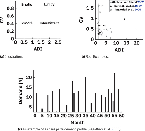
Subsequent research has produced thresholds for ADI and CV to produce a strategic chart consisting four demand types (Figure 1a) (A. Ghobbar & Friend, 2002). These are:

• Smooth demand ($\mathrm{ADI}<1.32$ and $\mathrm{CV}<0.49$) is regular in time and quantity making it easy to work with and has low error levels when forecasting.

• Intermittent demand ($\mathrm{ADI}\ge 1.32$ and $\mathrm{CV}<0.49$) has a history of no pattern, small variation in quantity but very high average intervals.

• Erratic demand ($\mathrm{ADI}<1.32$ and $\mathrm{CV}\ge 0.49$) features regular time occurrences with considerable quantity variations.

• Lumpy demand ($\mathrm{ADI}\ge 1.32$ and $\mathrm{CV}\ge 0.49$) has large quantity and time variations.

Figure 1b provides a set of real world examples and demonstrates where real world production exists within the space. While there are no limits on the maximum values for ADI and CV, the real-world systems reported to date typically operate between $0\le \mathrm{CV}\le 1$ and $0\le \mathrm{ADI}\le 5$.

Meeting smooth demand has been tackled through Just-in-Time and mass production practices. Intermittent demand has also seen considerable research with the development of batch manufacturing systems. Methods to co-ordinate and forecast manufacture across a manufacturing system include Croston’s method, model-based forecasting methods, bootstrapping and temporal aggregation (A. A. Ghobbar & Friend, 2003; Rožanec et al., 2022). The latter two demand types – Erratic and Lumpy – prove more difficult to plan for. Examples of these include job shops, bespoke & small-batch production, product maintenance/recalls, mass-customisation, and global ‘shock’ events (e.g. COVID) (Campbell, 1963; A. Ghobbar & Friend, 2002; J. A. Gopsill & Hicks, 2018; Mohan et al., 2019; Regattieri et al., 2005; Xie et al., 2019; Zhang et al., 2019)

The brief overview of the ADI-CV demand state space shows that it has been widely used across research and industry to characterise production demand and subsequently used to assess forecasting techniques. However, moving to on-demand production to meet these demand profiles imposes the additional factor of production time into the equation. Thus, modification to the computation of the ADI-CV demand state space is required.

2.2. Minimally intelligent agent-based manufacturing system modelling

Minimally Intelligent Agent-Based Manufacturing Systems is a concept where manufacturing machines can individually reason and decide their own strategies for processing jobs (J. Gopsill et al., 2022; Priore et al., 2001, 2014). The approach is diametrically opposed to the dominant industry practice of centralised manufacturing system control and governance.

Minimally Intelligent also refers to the ability to embed the capability on machine micro-controllers, which are resource-constrained and unable to deploy large Artificial Intelligent (AI) models, such as Deep Learning Neural Networks – at least in the near-term (Chung & Cheol-HeeYoo, 2013; Pantoja et al., 2018; Purusothaman et al., 2013). The vision also attempts to make the most use out of the compute resource available rather than require additional resource to operate (e.g. cloud high-performance computing).

Figure 2. Studies into minimally intelligent manufacturing systems.

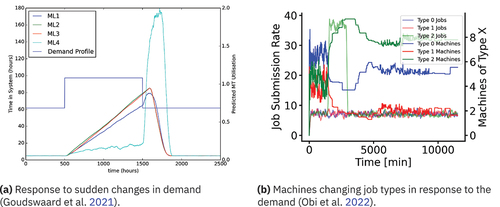
Through numerical modelling, Ma et al. (2021) showed minimally intelligent agent-based manufacturing systems to be more robust, resilient, and responsive compared to centralised control. Goudswaard et al. (2021) focused on sudden changes in demand behaviour with a numerical model of a minimally intelligent agent-based manufacturing system configured to handle a steady state demand input that then experienced a step, ramp, or saw-tooth change (Figure 2a). The study revealed that different configurations were required to respond effectively to different demand profiles.

Obi et al. (2022) demonstrated how agents with the minimal intelligence to switch job priority based on the composition of the incoming demand were able to respond to sudden changes in the distribution of job types being submitted (Figure 2b). Following the demand change, the system would slowly return to its original state, although some configurations resulted in more machines remaining on one type of job even though there was a steady-state stream of jobs equally distributed across the job types. The study highlighted that the configuration can affect the behavioural stability of the system and that it may not return to its original state post a demand spike.

2.3. Minimally intelligent agent-based manufacturing system implementations

Real-world implementations of Minimally Intelligent Agent-Based Manufacturing have also been gaining traction with developments in Industrial Digital Technology. Recent research has demystified the challenge of implementing an agent-based solution through the development of minimally intelligent enabled living labs (Giunta et al., 2022).

Figure 3 provides an overview of the implemented architecture.¹ The entire software stack was written in Typescript and used a tab in a Personal Computers (PCs) web browser to be the agent for a job or machine. In the case of a machine, a user would give permission for the browser window to access their 3D printer. A number of clients were produced that enabled printers to connect directly via USB, through intermediary software, such as Octoprint, or directly with the 3D printers own Application Programming Interface (API) (e.g. Ultimaker).

In the case of a job, the user would submit their gcode to the browser window where it would remain in their PCs RAM. The browser code would perform some analysis on the gcode to verify and access some details on the type of job (e.g. GCode flavour, print volume, material type, filament length required). The user would then connect their browser agent to the brokering service which was a server hosted in the cloud that co-ordinated agent messaging.

Figure 3. An example of a real-world implementation of an agent-based manufacturing system.

A figure illustrating a Minimally Intelligent Agent-Based Manufacturing System with tabs in a end-users web browser containing the agent that represents the machine/jobs in the system. These then connect to a broker server.

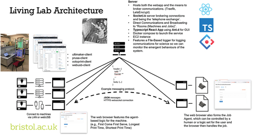
Encrypted websockets were used by the agents to send messages in real-time. The broker permitted agents to broadcast messages to populations/groups of agents as well as direct messaging. Different communication strategies could be deployed with different intelligences placed on the job and machine agents to negotiate and broker work. The negotiations featured only metadata with regard to the job and machine and only when a contract was struck was the gcode encrypted and sent to the agent representing the machine. The agent would then transmit the gcode to the connected machine.

Giunta et al. (2023) deployed the architecture on a set of machines in a lab setting and ran a series of accelerated job demand tests to examine the real-world viability of the approach as well as validating the numerical model used in this study. Ongoing work is building AI agents on a machines hardware as well as small low-powered devices, such as a Raspberry Pi.

Additional architectures have been proposed by the field and include an entirely cloud-based (Digital Shadow) approach where users configure their agents through a web browser but they actually co-exist in an application running in the cloud. When jobs are successfully brokered, the users would then connect their machine to receive the job. Entirely peer-to-peer services have also been proposed where there is a TURN/STUN server to initiate the connection between agents but no broker that could act as intermediary or validator for the messages being passed.

2.4. Smmary

In summary, the ADI-CV demand state space can be used to represent a broad range of demand scenarios with a considerable amount of past research mapping their demand profiles to the ADI-CV space. The four quadrants – smooth, intermittent, lumpy and erratic – have led to a collection of manufacturing system solutions and production planning methods. However, change in societal demand is driving on-demand manufacturing that introduces the additional factor of manufacturing time to the ADI-CV equation.

Research into Minimally Intelligent Agent-Based Manufacturing systems affords the re-configurability through the ability to change the intelligence of individual agents. Individual agents can act on behalf of single or multiple jobs and machines in a manufacturing system. While configurable, the emergent system behaviour and benefits in performance cannot be easily determined and require numerical simulation.

Further, moving to an on-demand manufacturing model to respond to demand across the ADI-CV demand space may also change the role of the Interval Review Period (IRP). Where it was previously defined based on how often decisions needed to be made concerning the re-stocking of spare parts, an on-demand manufacturing approach changes the decision as to which parts need to take priority. And in the case of agent-based manufacturing, IRP decisions may relate to the combination of agent intelligence in a network.

These findings led to the study presented in this paper that aimed to investigate and characterise the operating behaviours of Minimally Intelligent Agents for flexible manufacturing systems operating across the Average Demand Interval and Coefficient of Variation (ADI-CV) demand state space to assess their capability in meeting Big Demand.

3. Study design

The study used a numerical model to understand the operating behaviour of different configurations of minimally intelligent agent-based manufacturing systems across the ADI-CV demand state space. Given the ADI-CV represents four types of demand that range from intermittent single products to many thousands of products, there was no sensible means of testing them empircally. However, a select few points on in the ADI-CV demand state space were tested given the number of 3D printers in the lab and the data used the validate the numerical model. Please see Giunta et al. (2023) for the results.

The numerical model’s design consisted four steps:

1. Modifying the ADI-CV demand state space to account for manufacturing time.

2. Defining a set of ADI-CV demand state spaces to investigate.

3. Modelling a minimally intelligent agent-based manufacturing system to react to the different demand profiles.

4. Measuring the performance of minimally intelligent agent-based manufacturing system configurations.

Each of these steps are now discussed.

3.1. Modifying and parameterising the ADI-CV demand state space

Step 1 required modification and parameterisation of the ADI-CV Demand State Space in order to generate demand profiles for the minimally intelligent agent-based manufacturing system to handle. As mentioned in the Section 2, the existing ADI-CV demand state space does not account for the manufacturing time as it was originally intended to forecast required stock levels (i.e. manufacturing time is 0 and it is boolean as to whether the component is or is not in stock).

As the study considered on-demand manufacturing, it was deemed appropriate to adjust the ADI-CV demand state space calculation to account for the manufacturing time of products entering the system. Therefore, the position was taken to consider jobs as units of manufacturing time being submitted to the system and that the ADI-CV demand state space should represent the form in which the manufacturing time is submitted. For example, lots of small jobs vs one large job and smooth arrival vs intermittent arrival.

Through this lens, the ADI remains unchanged as it concerns only the arrival of jobs to the system. In contrast, CV had to be adapted to consider the distribution of manufacturing times that a job could arrive with. If this was not performed then a point on the ADI-CV could feature jobs with different distributions of manufacturing time thus making results difficult to interpret.

Recalling the original definition of CV:

(3) $\mathrm{CV}=\frac{\sqrt{(1/n){\sum }_{i=1}^n{\left({\epsilon }_i-{\epsilon }_a\right)}^2}}{{\epsilon }_a}$(3)

where ${\epsilon }_i$ is the job load at each time interval $\mathit{i}$, i.e. ${\epsilon }_i=J_i$ and ${\epsilon }_a$ is the mean job load over all time intervals, the modification involves defining the job load ${\epsilon }_i$ in terms of both the number of jobs and job durations. This defines each ${\epsilon }_i$ as the total added manufacturing time at time $t_i$. For each set of jobs, $J_i$, added at time $t_i$ with durations $T_j$, $\mathit{j}=1,\dots ,J_i$, the job load is then defined by ${\epsilon }_i={\sum }_{\mathit{j}=1}^{J_i}{T}_j$, and the CV definition becomes

(4) $\mathrm{CV}=\frac{\sqrt{(1/n){\sum }_{i=1}^n{\left({\sum }_{\mathit{j}=1}^{J_i}{T}_j-{\epsilon }_a\right)}^2}}{{\epsilon }_a}$(4)

where ${\epsilon }_a=(1/\mathit{n}){\sum }_{i=1}^n{\epsilon }_i$ is the average job load across all time intervals.

3.2. Defining a set of ADI-CV demand state spaces

Having redefined the ADI-CV demand state space, Step 2 involved defining the parameters used to systematically generate demand profiles across the ADI-CV demand state space. The parameterisation of the ADI-CV demand state space was reduced to three distributions:

1. An inter-arrival time distribution

2. An job quantity distribution

3. An job time distribution

To define a point on the ADI, inter-demand times $\mathrm{\Delta }{t}_i$ were assumed to be drawn from an integer uniform distribution with mean $T_c$ and spread $T_n$, $\mathrm{\Delta }{t}_i\sim \mathcal{U}\{T_c-(T_n-1)/2,T_c+(T_n-1)/2\}$. This distribution allows control over the mean and variance in the inter-demand period. The ability to set the average demand interval time using $T_c$ means that a desired periodicity in demand times can be generated. The parameter $T_n$ then defines a spread around this average value, to enable control over variability in demand interval times. The ADI is computed as the average inter-demand time $\mathrm{\Delta }{t}_i$, scaled by the Inter-Review Period (IRP), $\mathit{\tau }$.

The number of added jobs at each demand time, $J_i$, are assumed to be drawn from a shifted geometric distribution with parameter $\mathit{p}\in (0,1)$, that is $J_i\sim \mathrm{Geom}(\mathit{p})$. The shifted geometric distribution has mean $\mathit{\mu }=1/\mathit{p}$ and variance ${\sigma }^2=(1-\mathit{p})/p^2$. Hence, the CV of the shifted geometric distribution is given by $c_V^2={\mu }^2/{\sigma }^2=1-\mathit{p}$, meaning that demand profiles with a desired CV as defined in Equation (3)(3) $\mathrm{CV}=\frac{\sqrt{(1/n){\sum }_{i=1}^n{\left({\epsilon }_i-{\epsilon }_a\right)}^2}}{{\epsilon }_a}$(3) are generated by specifying the value of $\mathit{p}$. These two distributions were then combined with three job time distributions observed in manufacturing (Figure 4).

Figure 4. Three distributions of job duration.

A figure depicting three job time distributions – a constant job time, triangular distribution of job times and lognormal distribution of job times.

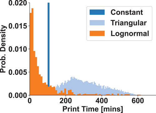
The first job time distribution featured constant job time, which, when set, would give the original ADI-CV demand state space, enabling the model to be validated against existing research and form a baseline for comparison. A constant job duration of 100 ($d_j=100$) was set as the value for the study. The second was a triangular distribution where a component with many variants that result in slight deviation from the most popular/standard variant (Goudswaard et al., 2021; Ma et al., 2021). A triangular distribution whose lower, upper, and middle job durations were set to 48, 600 and 240, respectively, was set. The third distribution was generated from Thingiverse’s catalogue of Additively Manufacturable products with the premise being that it represents what could be requested by consumers at any time (on demand). Job time data for components featured in the top 100 downloaded products was gathered from Thingiverse – a publicly available repository of 3D printable products (Baumann & Roller, 2018) – and fitted to a lognormal distribution, $T_j\sim \mathrm{lognormal}(\mathit{\mu }=3.5414,\mathit{\sigma }=1.3784)$. The dataset featured 996 components. Job times were calculated by slicing each of the components using the opensource Slic3r software which provided a manufacturing time estimation stored in the resulting gcode. Thus, the time represented a theoretical manufacturing time and did not consider variance as a result of custom machine settings that would override the gcode settings, the possibility of needing to change filament during the print or the process failing and needing to be restarted.

3.3. Minimally intelligent agent-based model

An agent-based approach was taken to model the minimally intelligent manufacturing system. Agents represent and act on behalf of elements within a system. In this case, the agent-based model featured two agent populations – Machine and Job – and a single Broker agent (Figure 5). Machine agents represent the machines and contain the necessary information to represent their manufacturing capability. Job agents represent the jobs that need to be manufactured and contain the necessary information for the job to be evaluated and manufactured by the machines. In this study, the machines were Additive Manufacturing machines of same capability and therefore capable of manufacturing any job entering the system (i.e. in a real-world system there would be validation checks that would prevent non-manufacturable jobs joining the system).

Figure 5. Agent-based model of a minimally intelligent agent-based manufacturing system.

A figure depicting an minimally intelligent agent-based manufacturing system where a series of Job and Machine agents connect to a Broker agent, which co-ordinates the exchange of messages between the agents. The Job and Machine agents negotiate to determine which job will be performed by which machine.

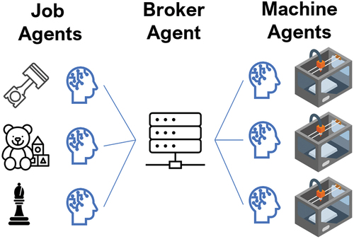
The Broker agent brokers connections and communication between the Machine and Job agents and is a representation of the network (e.g. cloud or local server) resources that would be required to maintain and facilitate communications.² The Broker permitted direct and broadcast communication. Communication was permitted between Machine – Job and Job – Machine. The negotiation strategy was set to co-ordinated manufacturing where the Machine agents lead the discussion and make the decisions, and Job agents are simply submissive providing the information requested by the Machine agents (J. Gopsill et al., 2022).

Figure 6. A typical communication exchange.

A figure depicting a typical communication exchange. Three vertical lines represent the Job Broker and Machine agent respectively. Horizontal lines depict the sender and receiver of a communication. Moving down the vertical lines depicts the order in which the communications are sent.

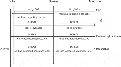
Figure 6 provides an overview of the communication protocol implemented in the model. A communication episode starts with a Machine agent that, if left idle for a period of time, would send a message to the Broker agent intended for all the Job agents connected to the network asking if the Job agent is available (machine_is_looking_for_available_jobs). The broker would then send the message to all the Job agents on the network. Job agents who are available respond with a directed message to the Machine agent (machine_is_available) with meta-information regarding the job it represents (e.g. job duration, volume, material type). These replies pass through the Broker to the Machine agent.

The Machine agent waits for a period of time to receive responses and after waiting, the Machine applies its intelligence to the list of responses to decide which job to select. If no jobs reply within the specified time then the Machine agent idles for a period of time before starting the process again. If a job is selected, the Machine agent issues a machine_has_chosen_a_job message to the relevant Job Agent.

The Job agent then replies has_accepted_offer or has_declined_offer. The Job agent would decline if it had been selected by another Machine agent in the time it took the Machine agent to decide and respond. If the Job agent accepts the Machine agents offer then the reply it sends also contains the manufacturing code for the Machine to start manufacturing. The Machine agent remains in a dormant state until the job is completed and a message is sent back to the Job agent to confirm that it has successfully been manufactured.

It was assumed that the flexible manufacturing technologies deployed in the system (e.g. Additive Manufacturing) was capable of manufacturing any of the jobs entering the system and that they achieved right first-time manufacture. Thus, the machine agents needed only to consider submission and manufacture time in their minimal intelligence deliberations. Five intelligences found in existing literature were used that considered submission and manufacture time:

• First Response First Serve (FRFS): Selects the first job that replies to its request.

• First Come First Serve (FCFS): Selects the job that was submitted earliest.

• Longest Manufacture Time (LMT): Selects the job with the longest print time.

• Shortest Manufacture Time (SMT): Selects the job with the shortest print time.

• Random: Randomly selects a job.

Job selection therefore becomes a function of the combination of agent intelligence, randomness in submission and polling time when machines were idle. The architecture affords considerable system configurability – $\mathit{m}\times \mathit{n}$ where $\mathit{m}$ is the number of machines and $\mathit{n}$ is the number of minimal intelligences.

The model was implemented in Rust³ and can be found at: https://github.com/zoharneu/BAMRust. A video tutorial describing the concepts of how to build the model can be found https://www.youtube.com/watch?v=NIVwWAGOLS8 list=PLAmnyJpQ2yBL0michF9OTisbyehZUrr8K pp=gAQBiAQB. The system was configured for continuous operation with the number of machines and their intelligence configured through a plain-text configuration file. The model has been validated in previous work through a Living Lab experiment involving a set of 3D printers each with an minimally intelligent agent installed tackling a uniform distribution of prints submitted throughout a day (Giunta et al., 2023).

3.4. Evaluating operating behaviour

Three metrics were used to assess the operating behaviour of different minimal intelligence combinations across the three ADI-CV demand state spaces. These were:

1. The stable operation boundary

2. The system responsiveness (Time-in-System)

3. The system overhead (message count)

The stable operation boundary metric assessed where the manufacturing system was stable or unstable. i.e. it was capable of meeting the demand placed upon it. This was measured by detecting the regions of the ADI-CV state space for which job load in the queue, $\mathit{L}={\sum }_k{d}_k$ for jobs $\mathit{k}$ in the queue, did not diverge. It was estimated by computing the derivative of the job load in the queue, $\mathrm{d}\mathit{L}/\mathrm{d}\mathit{t}$, and for a threshold $\mathit{\delta }>0$, a convergent performance by the condition $|\mathrm{d}\mathit{L}/\mathrm{d}\mathit{t}|<\mathit{\delta }$ was set. Systems that featured $|\mathrm{d}\mathit{L}/\mathrm{d}\mathit{t}|<\mathit{\delta }$ manage to reduce their total incoming job demand to a constant rate, while $|\mathrm{d}\mathit{L}/\mathrm{d}\mathit{t}|>\mathit{\delta }$ indicated an inability of the system to keep up with incoming job demand.

To estimate $\mathit{dL}/\mathit{dt}$, a derivative of the Savitsky-Golay method was used (Savitzky & Golay, 1964). The derivative involved fitting a LOWESS curve $\mathit{f}(\mathit{t})$ to the time-series of job load in queue, $\mathit{L}$, where 1/8th of the data was used to smooth the estimate at each point. The LOWESS curve was then differentiated to estimate $\mathrm{d}\mathit{f}/\mathrm{d}\mathit{t}\approx \mathrm{d}\mathit{L}/\mathrm{d}\mathit{t}$, and tested whether the estimate $\mathit{f}(\mathit{t})<\mathit{\epsilon }$ for the pre-defined threshold $\mathit{\epsilon }$, by averaging $\mathrm{d}\mathit{f}/\mathrm{d}\mathit{t}$ inside a given time window. $\mathit{\delta }=0.05$ was used. This gave the pass/fail criteria for the scenarios evaluated and was determined through visual inspection of job load when charted.

For stable system’s, the system responsiveness metric looked at the system’s ability to response to the demand. This was measured by the Time In System (TIS) experienced by jobs before they were selected by a machine:

(5) $\mathrm{TIS}=t_o-t_m-t_i$(5)

where $t_i$ is the time in, $t_o$ is time out and $t_m$ is manufacturing time. A system was considered responsive if the jobs flowing through the system featured low TIS.

The system overhead metric concerned the overhead in operating the manufacturing system. Agent-based systems are heavily Input/Output (IO) dependent and thus, the number of communications were examined. High message overheads are costly in terms of bandwidth and compute time in processing the messages. The tested message types include $m_{\mathit{M}1}$ (a broadcast of machine_is_looking_for_available_jobs), $m_{\mathit{J}2}$ (job_has_accepted_offer) and $m_{\mathit{J}3}$ (job_has_declined_offer). Broadcast messages are inherently IO heavy scaling linearly with the number of jobs on the networks. Equally the response to the broadcast can require equivalent bandwidth but is also a function of job availability. The acceptance message $m_{\mathit{J}2}$ contains the G-code for the job. So, while it is only sent to a single machine, the packet size is an order of magnitude larger (MBs rather than bytes) and if these messages happen to coincide then a bottleneck could be caused as they pass through the server. The rejection message $m_{\mathit{J}3}$ is an indicator of the competition for jobs between machines. Many rejections show that the system is not operating efficiently, with many instances of machines contending over jobs.

3.5. Numerical simulation

Six combinations of minimally intelligent agents were studied for a manufacturing system comprising 20 machines $N_m=20$. These were:

1. All FRFS

2. All FCFS

3. All LMT

4. All SMT

5. All Random

6. Mixed – consisting 4 LMT, 4 SMT and 12 Random machines.⁴

For each combination and job duration distribution, a parameter sweep of $T_c=[15,30,60,75,90,105,120]\mathrm{and}\mathit{p}=[0.01,0.1,0.2,0.3,0.4,0.5,0.6,0.7,0.8,0.9,\text{break}0.99]$ with $T_n=6$ and $\mathit{\tau }=60$. This resulted in 88 scenarios for each job time distribution across the ADI-CV demand state space − 264 scenarios in total. Each scenario was simulated for 30,000 time steps and repeated 60 times. Job demand profiles were randomly generated using different seeds for each simulation. A total of 15,840 simulations were performed.

The simulations were run on the University of Bristol’s High-Performance Computing platform – BlueCrystal. Post-processing and analysis of the simulations was performed locally using the Python packages Matploltib, Numpy, and SciPy (Harris et al., 2020; Hunter, 2007; Kluyver et al., 2016; Virtanen et al., 2020; Waskom, 2021).

4. Results

The results of the study are now presented in line with the three metrics of analysing system performance.

4.1. System stability

Figure 7. Stable system boundaries. The surf plot presents the relative ‘job loading’ on the system.

Three plots of the ADI-CV demand state space – one for each manufacturing time distribution profile. Lines on the plots depict where the manufacturing system transitions from stable to unstable operation.

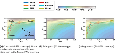
Figure 7 presents the stable operating regions of the six configurations of minimally intelligent agent manufacturing systems with respect to the three different manufacturing time distributions. In terms of constant manufacturing times (i.e. analogous to today’s spare part operations) (Figure 7a), the manufacturing systems maintain a steady-state operation across 85% of the state space. All combinations were equally stable across the state space and mapping the real-world cases onto the plot show that all but one could have been accommodated by a minimally intelligent system.

Moving to a triangular distribution of manufacturing times (Figure 7b), it can be seen that the region of stability becomes less comprehensive with the systems unable to handle the extremes of the Erratic, Lumpy and Smooth areas of the strategic chart (63% coverage). In terms of the extremity of Smooth demand, the system is moving to the realms of mass production where the system is simply unable to cope with the volume. In terms of Lumpy demand, there are occurrences where too many jobs enter the system at once and the system is unable to recover before the next wave of jobs. In the extreme of Erratic demand, there is a combination of both.

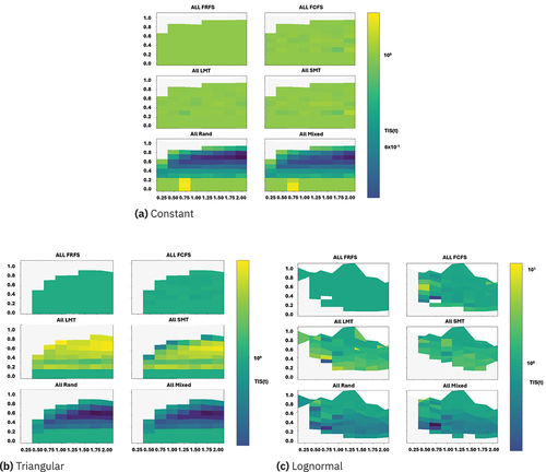
Figure 8. Average TIS for jobs in the converged regions normalised against FRFS.

Three subplots showing the difference in average TIS for the different logic configurations and the manufacturing time distribution. The all random and mixed logic configuration outperform the other logic configurations in responding to the three manufacturing time distributions across the ADI-CV demand state space.

Figure 7c shows the response of the system to a lognormal job distribution. This plot shows the system can operate over a greater range of the state space. Unlike the triangular distribution, many of the jobs are small and thus, do not ‘lock’ the system up for long periods of time. This distribution also exposes the limits of different intelligence combinations with some more stable than others with coverage ranging from 76–84% with the mixed and random combinations proving most stable and the LMT proving least stable.

4.2. System responsiveness

Figure 8 examines the stable operating regions for each of the six configurations across the three manufacturing time distributions and reports the cumulative TIS. The ALL FRFS has been used as the reference datum to compare the other configurations against. For constant manufacturing time, Figure 8a shows ALL FRFS, FCFS, LMT and SMT are similarly responsive. In contrast, ALL RANDOM and MIXED are shown to be more responsive with jobs spending less TIS. In the triangular distribution case (Figure 8b), ALL LMT and SMT perform worse than the datum for ALL FRFS across much of the state space while ALL RANDOM and ALL MIXED, again, prove to be the same or more responsive. In the lognormal case (Figure 8c), there is a less significant difference in the responsiveness of the system although the trend of ALL LMT and SMT generally performing worse and ALL RANDOM and ALL MIXED performing better exist.

4.3. System overhead

Figure 9. Total message counts versus total job load in the system. Note timeseries have been smoothed using a moving average.

Three sub-plots showing the correlation between the number of messages sent between the agents and job load in the system for the three different job distributions. All exhibit a tipping point where the message count suddenly rises as the system becomes unstable and is no longer able to cope with the demand.

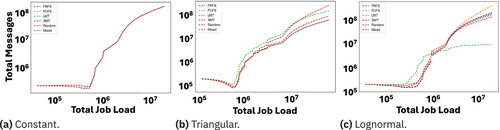
Figure 10. Relationships between message types for a different job duration distributions. [legend: • converged, • not converged].

Three subplots presenting the correlation matrix for different message types across the three job distribution. The points have been coloured coded to indicate whether the system was stable or unstable. The points cluster into groups that map to whether the system is stable or unstable.

Figure 9 shows the message count as a function of total job load across the three manufacturing distributions. Each follow a similar trend with a steady-state of messaging under a low job load. This would represent the typical pinging of requests for jobs by machines. As the systems reach capacity, the messaging starts to reduce with the machines spending more time manufacturing and less time communicating and bidding for work. Going beyond capacity, there is a sudden surge in messages and is a result of the many replies being sent by jobs and being received by the machines who can only handle one job at a time.

Figure 10 examines the relationship between message types being sent through the system. The stable and non-stable operations have been color coded orange and blue, respectively. In both the constant and lognormal distributions, there appears to be a single correlating point relating message types for stable operation. As the system becomes unstable the relationships move away from the point in a ‘fan’ style. In the triangular case, there are distinct message relationship regions that relate to stable and unstable operating regions.

5. Discussion

The results are now discussed where findings are highlighted and limitations and areas of future work are mentioned. Findings are highlighted FX and summarised in Table 1 at the end of the section. Table 1 also suggests whether the finding is of interest to industry, research or both.

5.1. Findings

The results have shown that minimally intelligent agent-based manufacturing systems can effectively resolve and operate across the ADI-CV state space observed and reported in literature. It suggests that manufacturers should not be concerned with transitioning to this type of operating model (F1). Minimally intelligent agent machines have been evidenced to self-organise to complete the incoming work no matter how smooth, intermittent, lumpy or erratic it is. Expanding the ADI-CV space calculations to factor in triangular and lognormal job distributions does limit their effectiveness at the extremes of the ADI-CV space for lumpy and erratic demands suggesting that those areas may still require bespoke solutions (F2). In the majority of cases, the combination of intelligence did not effect the limits of stable operation (F3). Rather, the combination of intelligence affected the system’s responsiveness to the demand with ALL RANDOM and ALL MIXED often providing reduction in job TIS (F4). The reason for this is that the random and mixed combination of intelligence removes the likelihood of machines competing for jobs. The impact can have a significant impact on TIS and thus, it is important to consider the combination of intelligence in order to maximise customer satisfaction.

The main operating overhead of a minimally intelligent agent-based manufacturing system is the degree of IO messaging passing through the broker. This has implications on broker server resource. The analysis of messages shows that, during stable operation, the message load remains fairly constant (F5). This has benefits in terms of a firm needing to only consider a fixed size (and cost) server to operate the system. In fact, it was observed that a system operating at near capacity reduces the message count thereby reducing the server requirements (F6). It could therefore be considered a ‘win, win’ to operate at near capacity.

It was shown that system instability can quickly be determined by monitoring message load with a sudden increase of messaging when a system goes unstable (F7). This can act as a warning system to prevent more jobs entering the network in order to return the system to a steady state. The relationships between message types had distinct features for both stable and unstable system operations, and again could be used to detect systems transitioning in and out of stability (F8). Further, these proxies require no analysis of the content of the messages and/or client IP (e.g. manufacturing code), which is advantageous for manufacturers wishing to operate such as system in IP sensitive sectors.

Table 1. A summary of the key findings from minimally intelligent agents operating across the ADI-CV space.

#	Finding	Relevance
1	Agent-based manufacturing systems can operate across the majority of the ADI-CV demand state space.	Industry
2	The manufacturing systems reach their limit in the extremities of lumpy and erratic demand.	Both
3	The combination of intelligence did not effect the stability of the system.	Both
4	The combination of intelligence did effect job TIS.	Industry
5	Messaging rates remain consistent and constant in stable systems enabling server to be sized and costs to be forecastable.	Industry
6	Systems operating at near capacity talk less.	Both
7	Message load suddenly increases when the system becomes unstable	Both
8	Monitoring the passing of message (without interrogating the content) can be used as a sensor for system performance	Research

5.2. Limitations and future work

The study was not without limitations and where opportunities for future work exist. The study assumed all machines could manufacture all jobs and this is unlikely to be the case in a real world setting where additional constraints such as build volume, material and work patterns (e.g. 9am-5pm, shifts, 24–7) exist. These additional constraints are likely to hamper the manufacturing systems in achieving the theorised throughput of jobs. The model can accommodate the addition of these constraints and thus, enables them to be explored in future work.

Further, no logistics were included in the model. It may be good to have your component manufactured in a day but if it is on the other side of the world then that might not be much use with delay introduced by the logistics of physically moving the components to their locations. Additional factors such as the carbon footprint need to also be considered to prove applicability and sustainability in real-world situations. These can be accommodated in an agent-based model through agents that represent the logistics of the supply chain. The progressive nature of agent-based solutions is another advantage of the approach enabling a firm to transform over a period of time and in sections.

The ADI-CV demand state space was not originally conceived with manufacturing times in mind. While it has been adapted in this paper in order to provide a point of comparison to existing literature, it may be more suitable to define a new demand state space for these future manufacturing systems and supply chains.

Avenues for future work also include determining the most appropriate ‘polling’ time for machines to look for jobs while not reducing the responsiveness of the system. This would effectively optimise the degree of messaging required for a desired responsiveness and further reduce the cost of operating the broker server. Different communication strategies need to also be considered where the owner of the job may wish to have a say in the decision-making and where the jobs and machines may need to come to a compromise and agree on a decision before manufacturing can commence.

6. Conclusion

Minimally Intelligent Agent-Based Manufacturing Systems have the potential to overcome the continued challenges in supply chain disruption and market fragility by enabling on-demand manufacturing. This study has examined their potential in operating across the ADI-CV demand state space. An established demand state space used by the aerospace, automotive and retail sectors. A numerical method was used to run simulations of six minimally intelligent manufacturing systems across an ADI-CV demand state with constant, triangular and lognormal job manufacturing time distributions. A total of 15,840 simulations were performed. The results were:

1. Minimally intelligent manufacturing systems can stably operate across 85%, 63% and 76-84% for the demand state spaces of constant, triangular and lognormal manufacturing time distributions, respectively, self-organising themselves to tackle the demand as it enters the system.

2. The configuration of logics does not effect the stable operating window.

3. The configuration of logics does effect job time-in-system and therefore customer satisfaction.

4. Messaging overhead is consistent for stable operations.

5. Monitoring high-level statistics of message count and message type correlations can provide indicators of stable and unstable system operation.

The results further support academic and industry literature suggesting agent-based manufacturing is a viable solution to the challenges being faced by global supply chains. In particular, the study determines the boundaries of capability which far exceed standard approaches and enables manufacturing to accommodate a wide range of demand.

Disclosure statement

No potential conflict of interest was reported by the author(s).

Data availability statement

Data relating to the publication can be regenerated by running the model stored in the repository – https://github.com/zoharneu/BAMRust.

Additional information

Funding

The work has been undertaken as part of the Engineering and Physical Sciences Research Council (EPSRC) grants – EP/R032696/1 and EP/V05113X/1 – and used the computational facilities of the Advanced Computing Research Centre, University of Bristol – http://www.bris.ac.uk/acrc/.

Notes

1. The code is opensource and can be found at https://github.com/jamesgopsill/bam-living-lab-broker and https://github.com/jamesgopsill/svelte-living-lab for the broker and client services, respectively.

2. Please see Giunta et al. (2023) for more information on a real-world implementation.

3. https://www.rust-lang.org/

4. Based on J. Gopsill et al. (2023) optimisation of Minimally Intelligent agent AM machines for Makerspaces.

References

- Baumann, F. W., & Roller, D. (2018). Thingiverse: Review and analysis of available files. International Journal of Rapid Manufacturing, 7(1), 83–25. https://doi.org/10.1504/IJRAPIDM.2018.089731
- Boylan, J. E., & Syntetos, A. A. (2009, November). Spare parts management: A review of forecasting research and extensions. IMA Journal of Management Mathematics, 21(3), 227–237. ISSN: 1471-678X. https://doi.org/10.1093/imaman/dpp016
- Brambilla, M., Ferrante, E., Birattari, M., & Dorigo, M. (2013). Swarm robotics: A review from the swarm engineering perspective. Swarm Intelligence, 7(1), 1–41. https://doi.org/10.1007/s11721-012-0075-2
- Campbell, H. S. (1963). The relationship of resource demands to airbase operations ( RM-3428-PR). Santa Monica: The Rand Corporation.
- Catapult, T. D. (2018). The Rise of Distributed Autonomous Manufacturing. https://www.digicatapult.org.uk/wpcontent/uploads/2021/11/The_rise_of_distributed_autonomous_manufacturing.pdf.
- Chung, I.-Y., & Cheol-HeeYoo, S.-J. O. (2013). Distributed intelligent microgrid control using multi-agent systems. Engineering, 5(1), 1–6. https://doi.org/10.4236/eng.2013.51b001
- Cliff, D. (2023). Parameterised response zero intelligence traders. Journal of Economic Interaction and Cooridination. https://doi.org/10.1007/s11403-023-00388-7
- Doussard, M., Schrock, G., Wolf-Powers, L., Eisenburger, M., & Marotta, S. (2018). Manufacturing without the firm: Challenges for the maker movement in three U.S. cities. Environment & Planning A: Economy & Space, 50(3), 651–670. https://doi.org/10.1177/0308518X17749709
- Forum, W. E., & Boston Consulting Group. (2021). Net-Zero Challenge: The Supply Chain Opportunity. World Economic Forum. https://www3.weforum.org/docs/WEF_Net_Zero_Challenge_The_Supply_Chain_Opportunity_2021.pdf
- Freitag, B., Häfner, L., Pfeuffer, V., & Übelhör, J. (2020). Evaluating investments in flexible on-demand production capacity: A real options approach. Business Research, 13(1), 2198–2627. https://doi.org/10.1007/s40685-019-00105-w
- Ghobbar, A. A., & Friend, C. H. (2003). Evaluation of forecasting methods for intermittent parts demand in the field of aviation: A predictive model. https://doi.org/10.1016/S0305-0548(02)00125-9
- Ghobbar, A., & Friend, C. (2002). Sources of intermittent demand for aircraft spare parts within airline operations. Journal of Air Transport Management, 8(4), 221–231. ISSN: 0969-6997. https://doi.org/10.1016/S0969-6997(01)00054-0
- Giunta, L., Hicks, B., & Gopsill, J. (2023). Creating a living lab software stack for validating agent-based manufacturing.
- Giunta, L., Obi, M., Goudswaard, M., Hicks, B., & Gopsill, J. (2022). Comparison of three agent-based architectures for distributed additive manufacturing. In: Procedia CIRP 107. Leading manufacturing systems transformation – Proceedings of the 55th CIRP Conference on Manufacturing Systems 2022, pp. 1150–1155. https://doi.org/10.1016/j.procir.2022.05.123.
- Gopsill, J., Goudswaard, M., Snider, C., Hicks, B., & Hicks, B. (2023). Automating makerspace and makerspace-like environment production: Optimal configurations of minimally intelligent agent-operated additive manufacturing machines. Artificial Intelligence in Engineering Design, Analysis and Manufacturing, 38. https://doi.org/10.1017/S0890060423000239
- Gopsill, J. A., & Hicks, B. J. (2018). Investigating the effect of scale and scheduling strategies on the productivity of 3D managed print services. Proceedings of the Institution of Mechanical Engineers, 232(10), 1753–1766. https://doi.org/10.1177/0954405417708217
- Gopsill, J., Obi, M., Giunta, L., & Goudswaard, M. (2022). Queueless: Agent-based manufacturing for workshop production. In G. Jezic, Y.-H.-J. Chen-Burger, M. Kusek, R. Šperka, R. J. Howlett, & L. C. Jain, Eds. Agents and multi-agent systems: Technologies and applications 2022. (pp. 27–37). Springer Nature Singapore: ISBN: 978-981-19-3359-2. https://doi.org/10.1007/978-981-19-3359-2_3
- Goudswaard, M., Gopsill, J., Ma, A., Nassehi, A., & Hicks, B. (2021,October). Responding to rapidly changing product demand through a coordinated additive manufacturing production system: A COVID-19 case study. In: IOP Conference Series: Materials Science and Engineering 11931, p. 012119. https://doi.org/10.1088/1757-899x/1193/1/012119.
- Gur, N., & Dilek, S. (2023, January). US–China economic rivalry and the reshoring of global supply chains. The Chinese Journal of International Politics, 16(1), 61–83. ISSN: 1750-8924: https://doi.org/10.1093/cjip/poac022
- Hamalainen, M., & Karjalainen, J. (2017). Social manufacturing: When the maker movement meets interfirm production networks. Business Horizons, 60(6), 795–805. ISSN: 0007-6813. https://doi.org/10.1016/j.bushor.2017.07.007
- Harris, C. R., Millman, K. J., van der Walt, S. J., Gommers, R., Virtanen, P., Cournapeau, D., Wieser, E., Taylor, J., Berg, S., Smith, N. J., Kern, R., Picus, M., Hoyer, S., van Kerkwijk, M. H., Brett, M., Haldane, A., Del Río, J. F., Wiebe, M. … Gohlke, C. (2020, September). Array programming with NumPy. Nature, 585(7825), 357–362. https://doi.org/10.1038/s41586-020-2649-2
- Hunter, J. D. (2007). Matplotlib: A 2D graphics environment. Computing in Science & Engineering, 9(3), 90–95. https://doi.org/10.1109/MCSE.2007.55
- Kikuchi, R., Yoshikawa, S., Jayaraman, P. K., Zheng, J., & Maekawa, T. (2018). Embedding QR codes onto B-spline surfaces for 3D printing. In: Computer-Aided Design 102. Proceeding of SPM 2018 Symposium, pp. 215–223. ISSN: 0010-4485. https://doi.org/10.1016/j.cad.2018.04.025.
- Kluyver, T., Ragan-Kelley, B., Pérez, F., Granger, B., Bussonnier, M., Frederic, J., Kelley, K., Hamrick, J., Grout, J., Corlay, S., Ivanov, P., Avila, D., Abdalla, S., & Willing, C. (2016). Jupyter notebooks – a publishing format for reproducible computational workflows. In F. Loizides & B. Schmidt (Eds.), Positioning and power in academic publishing: Players, agents and agendas (pp. 87–90). IOS Press.
- Kuncoro, E. G. B., Aurachman, R., & Santosa, B. (2018, November). Inventory policy for relining roll spare parts to minimize total cost of inventory with periodic review (R,s,q) and periodic review (R,S) (case study: PT. Z). IOP Conference Series: Materials Science and Engineering, 453(1), 012021. https://doi.org/10.1088/1757-899X/453/1/012021
- Kuuse, M. (2022). What is Distributed Manufacturing? http://manufacturing-software-blog.mrpeasy.com/distributed-manufacturing/.
- Luman, R., & Fechner, I. (2022, October). Trade Outlook 2023: Slow Steaming in Rough Water. https://think.ing.com/downloads/pdf/article/trade-outlook-slow-steaming-in-rough-waters-what-to-expect-in-2023.
- Ma, A., Nassehi, A., & Snider, C. (2021, January). Anarchic manufacturing: Implementing fully distributed control and planning in assembly. Production & Manufacturing Research, 9(1), 56–80. https://doi.org/10.1080/21693277.2021.1963346
- Mohan, J., Lanka, K., & Rao, A. N. (2019). A review of dynamic job shop scheduling techniques. In Procedia manufacturing 30. Digital manufacturing transforming industry towards sustainable growth (pp. 34–39). https://doi.org/10.1016/j.promfg.2019
- Nenni, M. E., Giustiniano, L., & Pirolo, L. (2013). Demand forecasting in the fashion industry: A review. International Journal of Engineering Business Management, 5, ISSN: 18479790. https://doi.org/10.5772/56840
- Obi, M., Snider, C., Giunta, L., Goudswaard, M., & Gopsill, J. (2022). Coping with diverse product demand Tthrough agent-led type transitions. In G. Jezic, Y.-H.-J. Chen-Burger, M. Kusek, R. Šperka, R. J. Howlett, & L. C. Jain Eds., Agents and multi-agent systems: Technologies and applications 2022. (pp. 277–286). Springer Nature Singapore.
- Ozturkcan, S. (2023). The right-to-repair movement: Sustainability and consumer rights. Journal of Information Technology Teaching Cases, 0.0. https://doi.org/10.1177/20438869231178037
- Pantoja, C. E., Soares, H. D., Viterbo, J., & Seghrouchni, A. E. F. (2018). An architecture for the development of ambient intelligence systems managed by embedded agents. The 30th International Conference on Software Engineering & Knowledge Engineering, San Francisco, July 1–3 (pp. 215–214). https://doi.org/10.18293/SEKE2018-110
- Papp, G., Hoffmann, M., & Papp, I. (2021). Improved embedding of QR codes onto surfaces to be 3D printed. Computer-Aided Design, 131, 102961. ISSN: 0010-4485. https://doi.org/10.1016/j.cad.2020.102961.
- Peckham, O., Goudswaard, M., Snider, C., & Gopsill, J. (2023). What to share? A preliminary investigation into the impact of information sharing on distributed decentralised agent-based additive manufacturing networks. In A. E. Romsdal, A. Strandhagen, J. O. von Cieminski, & D. Romero (Eds.), Advances in Production Management Systems. Production Management Systems for Responsible Manufacturing, Service, and Logistics Futures. APMS 2023 (Vol. 690). IFIP Advances in Information and Communication Technology. https://doi.org/10.1007/978-3-031-43666-6_36
- Pinçe, Ç., Turrini, L., & Meissner, J. (2021). Intermittent demand forecasting for spare parts: A critical review. Omega, 105, 102513. ISSN: 0305-0483. https://doi.org/10.1016/j.omega.2021.102513.
- Priore, P., De La Fuente, D., Gomez, A., & Puente, J. (2001). A review of machine learning in dynamic scheduling of flexible manufacturing systems. Ai Edam, 15(3), 251–263. https://doi.org/10.1017/S0890060401153059
- Priore, P., Gómez, A., Pino, R., & Rosillo, R. (2014). Dynamic scheduling of manufacturing systems using machine learning: An updated review. Ai Edam, 28(1), 83–97. https://doi.org/10.1017/S0890060413000516
- Purusothaman, S. R. R. D., Rajesh, R., Bajaj, K. K., & Vijayaraghavan, V. (2013). Implementation of Arduino-based multi-agent system for rural Indian microgrids. In: 2013 IEEE Innovative Smart Grid Technologies-Asia (ISGT Asia); pp. 1–5. https://doi.org/10.1109/ISGT-Asia.2013.6698751.
- Radius, F. (2021). Why Distributed Manufacturing is the Future of Production. http://www.fastradius.com/resources/distributed-manufacturing-benefits.
- Regattieri, A., Gamberi, M., Gamberini, R., & Manzini, R. (2005). Managing lumpy demand for aircraft spare parts. Journal of Air Transport Management, 11(6), 426–431. ISSN: 0969-6997. https://doi.org/10.1016/j.jairtraman.2005.06.003
- Remko, V. H. (2020). Research opportunities for a more resilient post-COVID-19 supply chain – closing the gap between research findings and industry practice. International Journal of Operations & Production Management, 40(4), 341–355. https://doi.org/10.1108/IJOPM-03-2020-0165
- Rožanec, J. M., Fortuna, B., & Mladenić, D. (2022). Reframing demand forecasting: A two-fold approach for lumpy and intermittent demand. Sustainability, 14(15), ISSN: 2071-1050. https://doi.org/10.3390/su14159295
- Savitzky, A., & Golay, M. J. E. (1964). Smoothing and differentiation of data by simplified least squares procedures. Analytical Chemistry, 36(8), 1627–1639. https://doi.org/10.1021/ac60214a047
- Tian, X., Wang, H., & Erjiang, E. (2021). Forecasting intermittent demand for inventory management by retailers: A new approach. Journal of Retailing and Consumer Services, 62, 102662. https://doi.org/10.1016/j.jretconser.2021.102662
- Virtanen, P., Gommers, R., Oliphant, T. E., Haberland, M., Reddy, T., Cournapeau, D., Burovski, E., Peterson, P., Weckesser, W., Bright, J., van der Walt, S. J., Brett, M., Wilson, J., Millman, K. J., Mayorov, N., Nelson, A. R. J., Jones, E., Kern, R. … Halchenko, Y. O. (2020). SciPy 1.0: Fundamental algorithms for scientific computing in python. Nature Methods, 17(3), 261–272. https://doi.org/10.1038/s41592-019-0686-2
- Walia, V., Byde, A., & Cliff, D. (2003). Evolving market design in zero-intelligence trader markets. In: EEE International Conference on E-Commerce, 2003. CEC 2003; pp. 157–164. https://doi.org/10.1109/COEC.2003.1210245.
- Waskom, M. L. (2021). Seaborn: Statistical data visualization. Journal of Open Source Software, 6(60), 3021. https://doi.org/10.21105/joss.03021
- Xie, J., Gao, L., Peng, K., Li, X., & Li, H. (2019). Review on flexible job shop scheduling. IET Collaborative Intelligent Manufacturing, 1(3), 67–77. 0009. https://doi.org/10.1049/iet-cim.2018.0009
- Zhang, J., Ding, G., Zou, Y., Qin, S., & Fu, J. (2019). Review of job shop scheduling research and its new perspectives under industry 4.0. Journal of Intelligent Manufacturing, 30(4), 1809–1830. https://doi.org/10.1007/s10845-017-1350-2