A self-learning framework combining association rules and mathematical models to solve production scheduling programs

ABSTRACT

Data-driven production scheduling and control systems are essential for manufacturing organisations to quickly adjust to the demand for a wide range of bespoke products, often within short lead times. This paper presents a self-learning framework that combines association rules and optimization techniques to create data-driven production scheduling. A new approach to predicting interruptions in the production process through association rules was implemented, using a mathematical model to sequence production activities in real or near real-time. The framework was tested in a case study of a ceramics manufacturer, updating confidence values by comparing planned values to actual values recorded during production control. It also sets a production corrective factor based on confidence value and success rate to avoid product shortages. The results were generated in just 1.25 seconds, resulting in a makespan reduction of 9% and 6% compared to two heuristics based on First-In-First-Out and Short Processing Time strategies.

KEYWORDS:

• Production scheduling and control
• association rules
• data-driven models
• big data analytics
• optimization techniques

1. Introduction

Current industrial environments are subject to multiple factors that influence manufacturing performance, such as machine breakdowns, variations of the orders production, fluctuation of demand, etc., potentially affecting the organisation’s resilience (Sanchis et al., 2021; Marcucci et al., 2022). According to the BCI Supply Chain Resilience Report (2023), during 2022, 11.5% of the organisations suffered more than ten disruptions, more than twice as much as pre-pandemic levels (4.8%). Respondents also stated that they estimated that their organisation experienced one to five incidents, which ultimately caused a significant disruption, notably affecting production efficiency. Moreover, these disruptions can also expand further within suppliers or retailers, snowballing in magnitude and worsening the impact on the resilience of the whole supply chain (Marcucci et al., 2023).

In this context, to maintain competitiveness among competitors, it is essential to be flexible and respond faster to variations in production planning. Every disruption in the production system can generate an inconsistency between the theoretical and the actual scheduling program. For this reason, the scheduling phase must be capable of predicting such anomalies to avoid errors in the delivery dates. Data Mining (DM) and Big Data Analytics techniques can play an essential role in the context of manufacturing production plans (Subramaniyan et al., 2018; Zafarzadeh et al., 2023; H. N. Zhang & Dwivedi, 2022) to predict production anomalies or disruptions. In particular, Association Rules (ARs) are a valuable tool to support decision-making processes and for discovering interesting hidden relationships in large data sets (Bala et al., 2010; Troncoso-García et al., 2023). ARs involve finding items or attributes that frequently occur together in a large dataset that satisfy two thresholds called min support and min confidence.

The present work aims to develop a framework that self-learns from past productions to prevent future production issues. This framework combines ARs and a mathematical model to establish a data-driven production scheduling that is capable of predicting non-conforming items based on several factors. A novel approach to the use of ARs is proposed based on different levels of accuracy, depending on the amount and type of data available. In particular, ARs are used to find relationships between various combinations of multidimensional antecedent variables (such as article code, type of material, number of parts to be manufactured, ambient humidity and temperature, etc.) and some consequent variables (production times, number of good parts, typology of defects, etc…). These consequent variables will be the input of scheduling processes. A mathematical model is proposed to solve the production scheduling problem, the Job-Shop Scheduling Problem (JSSP) and the Flow-Shop Scheduling Problem (FSSP). Thanks to the collaboration between ARs and the mathematical model, it is possible to have a scheduling plan that provides the global optimum solution to the problem and, at the same time, takes into account various factors influencing production. In addition, since the framework is based on the company’s historical data, the ARs solutions will become more accurate with each iteration.

In the literature, many scheduling models combine Artificial Intelligence (AI) techniques or DM approaches with heuristic methods to solve the scheduling problem (Y. Zhang et al., 2022). Although the existing research is valuable, a self-learning framework to structurally analyse and update real-time scheduling parameters by predicting relationships between multidimensional variables is not present in the literature to the best of the authors’ knowledge. For this reason, the scheduling framework proposed in this work aims to address this gap by introducing an innovative decision-making tool in this critical activity. A data-driven approach and a mathematical model were used to find a globally optimal solution to the problem of resource allocation in an unstable production environment.

The proposed framework was tested on a real case study to evaluate its accuracy. Implementing the proposed strategy aims to aid firms in adhering to the production scheduling program and, most significantly, the deadline for item delivery more consistently.

The manuscript is structured as follows: this introduction is followed by a literature review that analyses methods and objectives of data mining methodologies in scheduling problems (Section 2). Section 3 presents the research approach and framework, which is explained in detail, while the case study and the data set are described in Section 4. The discussion about theoretical contribution and practical implications are described in Section 5. To conclude, Section 6 summarises the paper and outlines future research directions.

2. Literature review

Research on scheduling problems has grown in recent years thanks to the development of Industry 4.0 solutions (Al-Banna et al., 2023; Salimbeni et al., 2023).

The scientific database Scopus has been chosen to conduct the literature review. Only English-language articles and conference papers published from 2019 to 2023 were selected to keep track of the latest contributions in literature. Every article has been reviewed to evaluate its pertinence and relevance to the theme established in this study. Table 1 shows the keywords used for the Scopus search and the publication number for each keyword pair.

Table 1. Keywords and number of publications.

Search in Article title, abstract and keywords	Papers found
“Job shop scheduling” AND “Association Rules”	2
“Flow shop scheduling” AND “Association Rules”	0
“Job shop scheduling” AND “Data Mining”	13
“Flow shop scheduling” AND “Data Mining”	3
“Job shop scheduling AND “Artificial Intelligence”	114
“Flow shop scheduling AND “Artificial Intelligence”	18

Looking at Table 1, it emerges that the use of DM techniques and ARs is not very widespread in the literature. Conversely, AI techniques are used in more significant numbers to approach the problem. The application of AI techniques for solving scheduling problems within a company is also closely related to the Smart Factory and Industry 4.0 concepts (Serrano-Ruiz et al., 2021) that have been spreading in recent years. Different AI techniques are used to solve the scheduling problem, but with other purposes, as Del Gallo et al. (2023) pointed out. Reinforcement Learning (RL) is widely used in the literature for solving the sequencing problem in dynamic and changing environments. An RL model that uses a Q-learning algorithm is introduced by Said et al. (2021) to solve a large-scale pharmaceutical factory scheduling problem. The proposed solution outperforms heuristic approaches such as first-in-first-out logic, both in terms of computation time and in terms of goodness of solution. Parameshwaran Pillai and Vijayan (2022) also suggested the Q-learning method, but in this instance, to solve two FSSPs in two different contexts. In both cases, a plastic toy factory and a core production plant, the algorithm outperformed the metaheuristic approach based on the PSO algorithm in terms of computation time and makespan value. Jing et al. (2022) exemplified a different approach, which proposed a multi-agent RL algorithm to solve a Flexible JSSP based on a Graph Convolutional Network. The solution was compared with three classic metrics (FIFO, Short Processing Time, and Long Processing Time) and with a dynamic RL algorithm, and the proposed solution generated the scheduling plan in a shorter time than the other methods it was compared. X. Wang et al. (2022b) offer a multi-agent RL approach to solve a Flexible FSSP problem by assigning workloads to 18 robot stations with different processing times. The Qmix algorithm was used to learn in the environment, outperforming other classic heuristic approaches and Distributed Agent Scheduling Architecture, which share the reward function among all agents. T. Zhou et al. (2021) implemented a combination of multi-agent RL and neural networks to solve a parallel machine scheduling problem in a robotic workstation. Unlike RL, Neural Networks (NN) are not used to solve the sequencing problem but to find complex features or correlations within data sets that are used to improve the scheduling plan and make it more accurate. Jacso et al. (2023) used artificial NN to simulate complex nonlinear relationships between key process factors and the observed data of surface quality and energy consumption. Several clever techniques, including Pattern Search, Genetic Algorithm, and Simulated Annealing, are used based on the optimised parameters to determine the best sequencing, configuration, and scheduling for several machines. There were two applications of the Simulated Annealing technique in the case study. While the second model alone optimises energy consumption, the first model seeks to maximise both energy consumption and makespan. Azab et al. (2021) created a system to forecast machine failure in scheduling programs by fusing machine learning techniques with commercial software solutions. A pharmaceutical business tried the suggested approach and several AI techniques; the findings indicate that the Decision Forest algorithm performed best, but the NN algorithm performed better in predicting the machine failure time.

However, using NNs often requires great computing power in the training phase, and the solutions they generate may be challenging to interpret. DM solutions are usually preferred, as in the case of Qiu et al. (2019), who conducted an experiment using data mining-based disturbance prediction for job shop scheduling. They used a hybrid algorithm to generate a disturbance tree, which was then used in the disturbance prediction module to construct a disturbance pattern, ensuring scheduling in the production process. Nasiri et al. (2019) propose a DM method that enhances the initial population for population-based heuristics for solving JSSP. They combine attribute-oriented induction (AOI) and ARs techniques, using a concept tree obtained from AOI as input for ARs. Here the ARs were used on a dataset of optimal or near-optimal solutions of a JSSP instance to identify associations between the attribute class of an operation and its sequence in the solutions. To evaluate the effectiveness of the proposed procedure, the authors used the solutions produced by the allocation procedure as the initial population for Genetic Algorithm and Particle Swarm Optimization to solve problem instances. Zhao et al. (2022) proposed a reactive scheduling method to deal with the uncertainty of new job arrival, using makespan and machine utilisation as scheduling criteria. The dynamic scheduling model assigns dispatching rules to sub-scheduling periods in real-time. Habib Zahmani and Atmani (2021) developed an approach that combines DM, Genetic Algorithm, and simulation techniques. DM is used to identify the best set of dispatching rules in a JSSP, while the Genetic Algorithm solves the JSSP by creating and evolving dispatching rule sets and assigning them to the shop floor’s machines. Y. Chen (2019) proposed a resource allocation algorithm based on big data association mining, which uses ARs extraction from big data and the adaptive scheduling approach for adaptive optimal control of resource allocation. L. Wang et al. (2022a) examined production lines using ARs and applied logic to resolve production rules between production lines and goods in the automobile manufacturing sector. Yang et al. (2022) realised a recognition method of delayed delivery risk transmission paths based on ARs and Bayesian networks. The first step involved determining ARs based on historical data and determining the Bayesian network topology structures of the risk transmission path. L. Zhou et al. (2019) built a mathematical model to solve a JSSP of a dynamic cloud manufacturing system. The model includes three single and three combined scheduling rules based on service time, logistics time, and subtask queue status of candidate services. Real-time information on tasks and services is used in the simulation strategy to select better scheduling rules.

Table 2 shows the analysed authors’ techniques and the scheduling problems they have encountered.

Table 2. Techniques and scheduling problems of the analysed publications.

	Techniques
AUTHORS	AI	DM	Self-learning	FSSP	JSSP
Qiu et al. (2019)		x			x
Nasiri et al. (2019)		x		x
Y. Chen (2019)		x		x
Said et al. (2021)	x		x		x
T. Zhou et al. (2021)	x		x	x
Azab et al. (2021)	x		x		x
Habib Zahmani and Atmani (2021)		x			x
Parameshwaran Pillai and Vijayan (2022)	x		x	x
Jing et al. (2022)	x		x		x
Zhao et al. (2022)		x		x	x
L. Wang et al. (2022a)		x		x
Yang et al. (2022)		x
X. Wang et al. (2022b)	x		x	x
Jacso et al. (2023)	x				x
Our solution		x	x	x	x

Compared to existing literature in the field, this paper fills a gap by proposing a production scheduling and control system based on a self-learning framework that exploits the advantages of DM. To the authors’ knowledge, our technique is unique in that it combines the accuracy of mathematical model results with the possibility of analysing production data in a lean and easily understandable manner using ARs.

Furthermore, while RL models look for a local optimum solution, the mathematical model allows for a global optimum solution to the problem and, thus, more accurate solutions. A novel use of ARs is proposed, utilising a level structure with varying degrees of accuracy dependent on the data at hand. Another novel aspect is the integration of DM techniques like ARs into a self-learning framework. Because of this, ever-better solutions are possible with limited processing power, and even non-expert users may quickly grasp the outcomes. Furthermore, the suggested architecture enables managers of the organisation to create new schedules and promptly modify existing ones in real-time or almost real-time.

3. Research approach

The general framework proposed in this paper comprises four phases, the first of which is ‘Data Management.’ This phase aims to gather the primary sources of the data-driven framework into a single database. Following this, ARs will be utilised to analyse the correlations between the various parameters of interest (‘Data Analytic phase’). The outcomes of this analysis will be incorporated into the data that is necessary for the execution of the scheduling plan and the optimisation of its performance (‘Optimization and Execution phase’). The ‘Control and Improvement phase’ is the final phase, primarily focusing on the self-learning processes. This is accomplished by capturing data from the manufacturing site and integrating it with the organisation’s management systems. The following sections will offer an overview of these four phases, and Figure 1 will exhibit a representation of the framework being presented.

Figure 1. Self-learning framework for scheduling program.

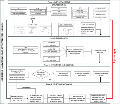
3.1. Step 1 – data management phase

The first step of the framework consists of collecting the different types of data of the company under investigation.

As highlighted in Figure 1, the aim is to integrate multiple data sources to create a single dataset to perform the analysis. To this end, it is necessary to know the existing data types (e.g. JSON, API, CSV, etc) and how they are collected. In Figure 1, a list of some of the most common information systems daily producing data is provided:

• Manufacturing Execution System (MES). Data related to the whole manufacturing process of the products realised are included in the MES, ranging from the activities performed by the personnel (e.g. workers involved, working hours, machinery parameters) to the parameters of the machines involved (such as machinery parameters provided through RFID, uptimes, and downtimes) and the material flow. These data must be collected and monitored in real time to gain insight into potential deviation from expected behaviour.

• Product Lifecycle Management (PLM). PLM is devoted to collecting and managing data regarding the whole lifecycle of products and processes. Such data are integrated into the MES.

• Programmable Logic Controller (PLC). PLC is used to continuously control production variables and machine states; such information is input into the MES.

• Supply Chain Management (SCM) system maps data regarding logistics activities with an external perspective: service levels, demand forecast and plan, resource optimisation and order processing.

• Other Data Set: all variables and datasets affecting production performance (ambient humidity and temperature, safety, maintenance info, etc.).

In the industrial context, data from the above sources must be pre-processed before the analysis. The Data Management step plays a crucial role in defining the overall quality of the framework. Failing to consider any inconsistencies during this phase can significantly influence subsequent procedures. Ensuring the accuracy of data collection, harmonising information from different sources and replacing missing values becomes imperative to provide a sound basis for subsequent analytical processes. These activities can be included in the Extraction, Transformation and Loading (ETL) process, which terminates with creating a unique dataset. In this way, a single data source can be analysed in the next phase through the use of ARs to extract the characteristics and relationships between the parameters collected in this phase.

3.2. Step 2 – data analytic phase

The Data Analysis phase aims to identify frequently occurring relationships between attributes and values in large datasets. In this phase, we use ARs to discover hidden connections in the dataset by establishing relationships between two sets of elements, known as antecedent and consequent. ARs generate simple rules such as ‘if X then Y’, which are easy to interpret. This is useful in obtaining a clear and intuitive understanding of the relationships between various attributes in the dataset. Such clarity can often be challenging with AI techniques, such as neural networks, which can be complex and difficult to interpret due to their intricate structure. Furthermore, extracting ARs generally requires less computing power than training complex artificial intelligence models, especially on moderate-sized datasets. Therefore, if resources are limited or computing time is a concern, Rules of Association are more appropriate.

3.2.1. Association rules

Association Rules mining is a technique applied to analyse transactions in a dataset to discover co-occurrence patterns between elements. Specifically, frequent itemsets are considered in the ARM procedure, i.e. sets of items appearing concurrently with a frequency higher than a specific threshold.

Let us consider an implication in the form: x$\to \mathit{\hspace{0.17em}}$y:

• X and Y are frequent itemsets extracted from the dataset.

• X is called the ‘antecedent’ of the rule, while Y is the ‘consequent’.

• X and Y have no items in common (i.e. X ∩ Y= ∅).

The antecedent represents the condition that generates an event, result, or outcome, which in the context of ARs is called consequent.

The quality of an AR x $\to$ y can be evaluated using a variety of measures. The support (Supp) and confidence (Conf) are used in this work.

• Supp(x$\to$y) = $\{(\mathit{x},\mathit{y})\}\text{overm}$. The support of a rule is the probability of simultaneously finding itemset x and y in an instance of the dataset; hence, it can be calculated by dividing the number of instances both containing {(x, y)} by the cardinality of the dataset itself (m).

• Conf(x$\to$y) =$\frac{\mathrm{Supp}\left(\mathrm{x}\to \mathrm{y}\right)}{\mathrm{Supp}\left(\mathrm{x}\right)}$. Confidence indicates the probability of finding item y in a row of the dataset that contains item x.

ARM can be carried out as a two-step process:

1. Frequent itemset extraction: items that appear more frequently than a user-defined threshold are extracted from the dataset. Such threshold is generally called minimum support. The algorithm used to this end is the Apriori (Agrawal & Srikant, 1994): it identifies the frequent itemset within the dataset through a pruning strategy, aiming to remove infrequent itemsets and reduce the number of iterations, thus improving calculation performance.

2. ARs definition: for each frequent itemset (G) extracted at step (a), all rules x$\to \mathit{\hspace{0.17em}}$y are generated so that x U y = G. The cut-off value for rule generation is the minimum confidence: rules having confidence lower than such value, will not be taken into account for the analysis.

Several authors pointed out that ARs are easy to interpret and follow an intuitive pattern, making the algorithm’s outputs understandable even to non-technical users (e.g. Antomarioni et al., 2022; Crespo Márquez et al., 2019). Furthermore, the Apriori algorithm is effective in handling large transactional datasets. Thanks to its pruning strategy based on the concept of ‘support’, the algorithm eliminates combinations that do not satisfy a certain frequency level, helping to reduce computational complexity.

Table 3 reports an example of a dataset in which it is possible to use ARs to extract useful information. In this example, each row represents a production process conducted in a specific machine (e.g. Machine 1), and it reports information about the type of product realised, the supplier and the percentage of good parts realised. It should be noted that the instances included in Table 3 are used to help clarify the rationale followed to extract the ARs.

Table 3. Example of potential input dataset for ARs extraction.

ID	Items (Product ID, Supplier ID, Machine ID, % of good part realised)
1	Product 1, Supplier 2, Machine 1, 100%
2	Product 2, Supplier 1, Machine 1, 100%
3	Product 3, Supplier 2, Machine 1, 80%
4	Product 2, Supplier 4, Machine 1, 100%
5	Product 1, Supplier 2, Machine 1, 50%
6	Product 1, Supplier 2, Machine 1, 100%

Assuming the percentage of good parts as the consequent and the Product ID, the Supplier ID and the Machine ID as antecedents. If a production manager is interested in determining the probability of producing 100% of good parts of Product 1 on Machine 1 using materials purchased from Supplier 2, then the rule (Product 1, Supplier 2, Machine 1) ➔ 100% should be extracted. The probability measure will then be determined by calculating Supp and Conf metrics. Specifically: Supp ((Product 1, Supplier 2, Machine 1) ➔ 100%) = 33,3%. This means that in the dataset (Table 3), 33, 3% (2/6) of the rows contain the information (Product 1, Supplier 2, Machine 1, 100%).

• Conf ((Product 1, Supplier 2, Machine 1) ➔ 100%) = 66,7%. This means that considering only the instances containing Product 1, Supplier 2, and Machine 1, the probability of finding 100% of good parts is 66,7%.

So, in conclusion, if a batch of Product 1 on Machine 1 has to be realised with materials supplied by Supplier 2, there will be a 66,7% chance of producing all good parts.

3.2.2. Association rules application

From the best of the authors’ knowledge, in our framework, we propose an innovative use of ARs for the extraction of features or correlations useful for the realisation of more accurate scheduling plans. In particular, the variables selected as antecedents are the ones whose value may imply a variation on the consequent ones. For instance, since the main objective of the proposed framework is developing a scheduling plan, information like job processing time, setup time, quantity and % of good parts are the ones on which the attention should be focused. Moreover, it should also be considered that the abovementioned values may vary depending on the type of material, supplier or article produced. Hence, consequents are selected taking into account all parameters which are fundamental to developing a production scheduling plan as an input (job duration, % of good parts, setup times, quantity to be produced, etc.); on the other end, the antecedents are taken from all other parameters that could help predict the identified consequents (i.e. type of raw materials to be worked, type of article to be produced, type of suppliers, type of machines to be used, …).

Different antecedent parameters characterise every production process. These parameters can be classified into two groups:

• m constant parameters that describe some attributes that never change during a period from the scheduling

• n variable parameters that may change from one machining operation to the next (Month, Number of parts to be produced, type of raw materials, etc.).

Variable parameters may only be available from one program to the next, for example, because the company needs information on the characteristics of raw materials. However, as the proposed framework is a general roadmap adaptable to different kinds of companies and contexts, it must function even without such information. For this reason, various levels of ARs were created depending on the number of variable parameters. Constant and variable parameters will form groups of ARs made up of m + i parameters as antecedents, with i∈[1,n]. For every consequent variable, several groups of ARs can be defined according to the number of antecedent parameters we considered. An Association Rules Level (ARL) is a group of ARs that have the same number of variable parameters as the antecedent. It is possible to have more than one AR for a specific level according to the potential combination of antecedent parameters.

So, it is possible to define:

• Association Rules Level 1 (ARL1) is the set of rules that have m + n parameters as antecedents.

• Association Rules Level 2 (ARL2) is the set of rules that have m + (n-1) parameters as antecedents.

• …

• Association Rules Level n (ARLn) is the set of rules with m + 1 parameters as antecedents.

The classification of ARs at different levels helps to find more rules which describe the process with different levels of accuracy. This aspect ensures that, when the company has to schedule a new JOB, we could connect that JOB to n, n-1 or only 1 variable parameter, depending on the information we have available for that JOB. Due to the lack of historical data, it may not be possible to associate all n variable parameters as antecedents to a task. The framework guarantees operation even without specific variable parameters thanks to the level structure.

The higher the number of parameters selected as antecedents, the more accurate the process description will be. The itemset used to define the rules at the ARL1 level will consist of (m+n) variables as antecedents plus the consequent (e.g. production times, number of good parts, typology of defects, etc.).Otherwise, we will progressively use the itemsets with fewer antecedents (ARL2, ARL3, …, ARLn).

Figure 2 shows the scheme followed to search for ARs related to a given JOB. Each task to be scheduled will initially be compared with the results of the ARL1 to search for a rule describing the task to be scheduled. If, among the ARL1s, there are one or more groups of antecedents that describe the process to be scheduled, then the consequent values will be extracted with the rule’s relative support and confidence values. Otherwise, it will proceed iteratively by searching for rules in subsequent levels.

Figure 2. Investigating the correlation between the outcomes generated by ARs and the sequence of operations to be scheduled.

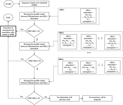
In detail, let us consider that k constant parameters (m₁, m₂, … , m_k) and i variable parameters (n₁, n₂, …, n_i) are provided for each scheduling plan. In the first step, the JOB to be scheduled is compared with the antecedents of ARL1. If all k+i parameters are available for that JOB, then a set of rules characterising the production process among the itemsets of ARL1 will be used, and support and confidence values will be calculated and extracted. If there are no rules describing the process to be scheduled, then the JOB parameters are compared with the lower level (ARL2). The ARL2 consists of several groups of itemsets, one for each possible combination of variable parameters. Again, the JOB to be scheduled are compared with the itemsets in the different ARL2 groups, and if a correlation exists, the support and confidence values are extracted. Possible matches will be evaluated on the lower level if no relationship between JOB parameters and antecedents is found. This process iterates up to the last ARL level, where only one variable parameter is considered to characterise the process. If no antecedent groups describing the process are found even at the previous level, there are no similar processes in the data history. In that case, the company operators estimate the consequent ‘c’ according to their experience. Figure 2 shows the procedure to be followed during the Data Analytics phase to extract the ARs considering m_k possible constant parameters and n_i possible variable parameters as antecedents.

3.3. Step 3 - optimization and execution phase

The third step of the framework is the optimisation and execution of the scheduling plan. The optimisation phase can be focused on different objectives. Several optimisation algorithms can be used for this purpose. In the case study analysed in the next section, the objective was the minimisation of the production makespan. The makespan is a metric used in task scheduling and planning problems, and it indicates the total amount of time required to complete all jobs. The proposed scheduling algorithm turns out to be flexible for both FSSP and JSSP. FSSP and JSSP are known as NP-hard problems (Babor et al., 2023). There was a limited availability of resources for processing, and each machine had its own matrix setup time. Table 4 illustrates all the parameters and variables describing the mathematical model for solving the scheduling problem.

Table 4. Problem parameters and decision variables.

Index	Description
Problems Parameters
J	Set of n jobs to be realized {j1, j2, …, jn}
$\mathit{j}$	Unique identifier for each job to be scheduled
M	Set of s machines {m1, m2, …, ms}
$\mathit{m}$	Unique identifier for each machine involved in the programming process
O	Set of z materials available {o1, o2, …, oz}
$\mathit{o}$	Unique identifier for each material used in production work
Q	Set indicating all jobs with a progress status > 0 {q1, q2,…, qb}
$\mathit{q}$	Unique identifier for each job with a progress status > 0
T	Set of set-up times for a machine {T1, T2, … , Ts}
$\mathit{t}\left(j^{\prime },\mathit{m},o^{\prime },j^{\prime \prime },o^{\prime \prime }\right)$	Setup time to switch from the production of $\left(j^{\prime },\mathit{m},o^{\prime }\right)$ to the production of $\left(j^{\prime \prime },\mathit{m},o^{\prime \prime }\right)$
$\mathit{prec}\left(\mathit{j},\mathit{m}{ }^{\mathrm{\prime \prime }},\mathit{o}\right)$	Represents the precedence relation between (j, m’, o) and $\left(\mathit{j},m^{\prime \prime },\mathit{o}\right).$
Decision Variables
$\mathit{dur}\left(\mathit{j},\mathit{m},\mathit{o}\right)$	Duration of job j on machine m with material o
$\mathit{start}\left(\mathit{j},\mathit{m},\mathit{o}\right)$	Time to start job j on machine m with material o
$\mathit{dur}\left(\mathit{q},\mathit{m},\mathit{o}\right)$	Duration of job q on machine m with material o
$\mathit{start}\left(\mathit{q},\mathit{m},\mathit{o}\right)$	Time to start job q on machine m with material o

A typical scheduling problem is described by allocating a set of jobs J to a group of machines M, and the various jobs to be manufactured can be made up of different materials O.

The single task to be scheduled is characterised by the tern $\left(\mathit{j},\mathit{m},\mathit{o}\right):$ job $\mathit{j}$ with material $\mathit{o}$processed on the machine m. If an activity is in progress on a specific job during the start of a new scheduling programme, it cannot be interrupted. For this reason, this operation must be the first to be scheduled. When the scheduling plan is launched, jobs with a completion percentage greater than zero will be indicated with the index $\mathit{q}$ of the set Q and the activity with the tern $\left(\mathit{q},\mathit{m},\mathit{o}\right).$ Moreover, different set-up times have been considered for every job and machine. These are the set-up times necessary to pass from job j with material o to another job with different material in the machine m for every $\left(\mathit{j},\mathit{m},\mathit{o}\right)$ to be scheduled.

The optimisation problem aims to minimise the makespan value; therefore, the objective function is expressed by equation (1)(1) $\mathit{minimize}\left(\mathit{makespan}\right)=\mathit{minimize}(max\{\mathrm{\forall }\mathit{x}\in \mathit{R}|\mathit{x}=\mathit{start}\left(\mathit{j},\mathit{m},\mathit{o}\right)+\mathit{dur}\left(\mathit{j},\mathit{m},\mathit{o}\right),\mathrm{\forall }\left(\mathit{j},\mathit{m},\mathit{o}\right)$(1) :

(1) $\mathit{minimize}\left(\mathit{makespan}\right)=\mathit{minimize}(max\{\mathrm{\forall }\mathit{x}\in \mathit{R}|\mathit{x}=\mathit{start}\left(\mathit{j},\mathit{m},\mathit{o}\right)+\mathit{dur}\left(\mathit{j},\mathit{m},\mathit{o}\right),\mathrm{\forall }\left(\mathit{j},\mathit{m},\mathit{o}\right)$(1)

(2) $\mathit{start}\left(\mathit{j},\mathit{m},\mathit{o}\right)\ge 0\mathrm{\forall }\left(\mathit{j},\mathit{m},\mathit{o}\right)$(2)

(3) $\mathit{dur}\left(\mathit{j},\mathit{m},\mathit{o}\right)\ge 0\mathrm{\forall }\left(\mathit{j},\mathit{m},\mathit{o}\right)$(3)

(4) $\mathit{start}\left(\mathit{j},\mathit{m},\mathit{o}\right)+\mathit{dur}\left(\mathit{j},\mathit{m},\mathit{o}\right)\le \mathit{makespan}\forall \left(\mathit{j},\mathit{m},\mathit{o}\right)$(4)

(5) $\mathit{start}\left(\mathit{j},\mathit{m}{ }^{\mathrm{\prime }},\mathit{o}\right)+\mathit{dur}\left(\mathit{j},\mathit{m}{ }^{\mathrm{\prime }},\mathit{o}\right)\le \mathit{start}\left(\mathit{j},\mathit{m}{ }^{\mathrm{\prime \prime }},\mathit{o}\right)\mathrm{\forall }\left(\mathit{j},\mathit{m}{ }^{\mathrm{\prime }},\mathit{o}\right)=\mathit{prec}\left(\mathit{j},\mathit{m}{ }^{\mathrm{\prime \prime }},\mathit{o}\right)$(5)

(6) $\mathit{start}\left(\mathit{q},\mathit{m},\mathit{o}\right)+\mathit{dur}\left(\mathit{q},\mathit{m},\mathit{o}\right)\le \mathit{start}\left(\mathit{j},\mathit{m},\mathit{o}\right)$(6)

$\mathit{start}\left(\mathit{j}{ }^{\mathrm{\prime }},\mathit{m},\mathit{o}{ }^{\mathrm{\prime }}\right)+\mathit{dur}\left(\mathit{j}{ }^{\mathrm{\prime }},\mathit{m},\mathit{o}{ }^{\mathrm{\prime }}\right)+\mathit{t}\left(\mathit{j}{ }^{\mathrm{\prime }},\mathit{m},\mathit{o}{ }^{\mathrm{\prime }},\mathit{j}{ }^{\mathrm{\prime \prime }},\mathit{o}{ }^{\mathrm{\prime \prime }}\right)\le \mathit{start}\left(\mathit{j}{ }^{\mathrm{\prime \prime }},\mathit{m},\mathit{o}{ }^{\mathrm{\prime \prime }}\right)$

(7) $\mathit{start}\left(\mathit{j}{ }^{\mathrm{\prime \prime }},\mathit{m},\mathit{o}{ }^{\mathrm{\prime \prime }}\right)+\mathit{dur}\left(\mathit{j}{ }^{\mathrm{\prime \prime }},\mathit{m},\mathit{o}{ }^{\mathrm{\prime \prime }}\right)+\mathit{t}\left(\mathit{j}{ }^{\mathrm{\prime \prime }},\mathit{m},\mathit{o}{ }^{\mathrm{\prime \prime }},\mathit{j}{ }^{\mathrm{\prime }},\mathit{o}{ }^{\mathrm{\prime }}\right)\le \mathit{start}\left(\mathit{j}{ }^{\mathrm{\prime }},\mathit{m},\mathit{o}{ }^{\mathrm{\prime }}\right)$(7)

Equations (2)(2) $\mathit{start}\left(\mathit{j},\mathit{m},\mathit{o}\right)\ge 0\mathrm{\forall }\left(\mathit{j},\mathit{m},\mathit{o}\right)$(2) and (3(3) $\mathit{dur}\left(\mathit{j},\mathit{m},\mathit{o}\right)\ge 0\mathrm{\forall }\left(\mathit{j},\mathit{m},\mathit{o}\right)$(3) ) specify non-negative numbers for the duration and start time. With equation (4)(4) $\mathit{start}\left(\mathit{j},\mathit{m},\mathit{o}\right)+\mathit{dur}\left(\mathit{j},\mathit{m},\mathit{o}\right)\le \mathit{makespan}\forall \left(\mathit{j},\mathit{m},\mathit{o}\right)$(4) , the end time of a single activity must be less than the makespan. Equation (5)(5) $\mathit{start}\left(\mathit{j},\mathit{m}{ }^{\mathrm{\prime }},\mathit{o}\right)+\mathit{dur}\left(\mathit{j},\mathit{m}{ }^{\mathrm{\prime }},\mathit{o}\right)\le \mathit{start}\left(\mathit{j},\mathit{m}{ }^{\mathrm{\prime \prime }},\mathit{o}\right)\mathrm{\forall }\left(\mathit{j},\mathit{m}{ }^{\mathrm{\prime }},\mathit{o}\right)=\mathit{prec}\left(\mathit{j},\mathit{m}{ }^{\mathrm{\prime \prime }},\mathit{o}\right)$(5) imposes that an activity cannot begin if the activity that preceded it has not been completed; it refers to those activities subject to precedence constraints with other activities. Meanwhile, equation (6)(6) $\mathit{start}\left(\mathit{q},\mathit{m},\mathit{o}\right)+\mathit{dur}\left(\mathit{q},\mathit{m},\mathit{o}\right)\le \mathit{start}\left(\mathit{j},\mathit{m},\mathit{o}\right)$(6) gives precedence to work in progress during the execution of the new scheduling plan; this is because it was assumed that a job cannot be interrupted if it has already started.

A disjunction equation is a type of equation that contains at least two expressions separated by the word ‘or’. The objective of solving a disjunction equation is to find all values that satisfy at least one of the two equations separated by the term ‘or’. Equation (7)(7) $\mathit{start}\left(\mathit{j}{ }^{\mathrm{\prime \prime }},\mathit{m},\mathit{o}{ }^{\mathrm{\prime \prime }}\right)+\mathit{dur}\left(\mathit{j}{ }^{\mathrm{\prime \prime }},\mathit{m},\mathit{o}{ }^{\mathrm{\prime \prime }}\right)+\mathit{t}\left(\mathit{j}{ }^{\mathrm{\prime \prime }},\mathit{m},\mathit{o}{ }^{\mathrm{\prime \prime }},\mathit{j}{ }^{\mathrm{\prime }},\mathit{o}{ }^{\mathrm{\prime }}\right)\le \mathit{start}\left(\mathit{j}{ }^{\mathrm{\prime }},\mathit{m},\mathit{o}{ }^{\mathrm{\prime }}\right)$(7) describes the behaviour whereby if a machine is engaged in a machining operation, it cannot start an activity of another item until the previous activity has been completed. Thanks to this expression, overlapping the activities in the scheduling program is impossible.

Regarding the availability of machines, it is necessary to introduce a machine availability calendar that states day by day what is working or not working time and the available working hours for every machine.

After the optimisation phase, the scheduling plan will be provided to the operation managers to be executed.

3.4. Step 4 - control and learning phase

Within the context of production control, this step involves comparing the actual and expected values used throughout the process of developing the scheduling planning plan. The Data Management phase involves collecting actual data in the production sector using various techniques determined by the company’s management system.

The organisation can discern discrepancies between realised and planned values and identify corrective measures to incorporate into the following scheduling plans by comprehensively comparing planned and actual parameters. The comparative analysis allows the identification of deviations between planned and realised parameters. All the corrective measures identified will be incorporated into the database used for the antecedents and subsequently used in data processing. This strategic integration facilitates the creation of a self-learning methodology. Leveraging the results of the process, the data set can be expanded with additional data from production procedures. This iterative improvement ensures a progressive system refinement, culminating in the closing of the self-learning cycle.

4. Case study

The proposed framework was tested on a real case study of a medium-sized manufacturing company. The company is focused on producing ceramic sinks of different sizes and forms and with different ceramic types. The ceramic used by the company is a mixture of various raw materials, and it is a critical aspect of the production process because it is vulnerable to several variables, such as room temperature, air humidity, and other parameters.

The ceramic sinks’ production process comprises ten steps, as shown in Figure 3.

Figure 3. Production process of ceramic sinks.

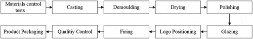
In Table 5, a short description of the production processes is reported.

Table 5. Sequence of the production process.

#Process	Production process	Description
1	Materials control tests	Before the casting process, the clay’s quality is checked, particularly its thixotropy, viscosity, density and temperature. If the clay is unsuitable for casting, modifications are applied, and after 30 minutes, the test will be repeated. The glazing operator checks the glaze daily; tests are carried out to measure viscosity and density.
2	Casting	The casting operator makes the moulds, considering the demoulding times according to the results of the clay thixotropy test.
3	Demoulding	The casting operator opens moulds; the de-moulding plate will be applied at the base of the sinks. Then, rectifying structures are put inside sink bowls to stay.
4	Drying	After demolding, a stamp with the casting date is applied to the bottom of the pieces. Then, the pieces are placed in the dryer.
5	Polishing	The parts are taken from the dryer and brought to the polishing cabin, where the operator finishes each part.
6	Glazing	After polishing, the operator picks up the pieces and applies the engobe (glaze base) and the glaze.
7	Logo Positioning	A laser-tech tool has been projected for this task.
8	Firing	The operator unloads the previous kiln charge, cleans the kiln carriage with a vacuum, applies engobe on the carriage panels and charges the new coming pieces to be fired; then the firing process can start. Therefore, this process can generate several defects and is considered the most critical in the production chain.
9	Quality Control	The quality control manager must check all the unloaded pieces and report all the results in a data sheet to see if they comply with standards.
10	Product Packaging	The controlled products are packed by an operator into their respective boxes, labelled and placed on pallets.

The proposed framework is used in this case study to develop a daily production scheduling program to predict product defects, re-schedule the program if the company MES highlights a variance between the real and planned non-compliant products, and self-learn from previous programs.

The following sub-sections will present the different framework phases concerning the case study.

4.1. Data management phase

An extract of the data used by the company to make the schedule is shown in Table 6. Info is collected from different data sources (MES, PLM, SCM). Each operation is characterised by several factors: type of product, type of process, type of raw material, job duration, precedence constraints, customer demand and completion percentage. For reasons of company confidentiality, the names of the articles and ceramics used have been generalised.

Table 6. List of tasks that must be scheduled.

#JOB	JOB characteristics (product ID, machine type, ceramic type)	Duration [min]	Prerequisite (precedence constraints)	Demand	%complete
1	(‘Product 1’, ‘Material tests’, ‘Cer 1’)	10	None	30	10
2	(‘Product 1’, ‘Casting’, ‘Cer 1’)	16	(‘Product 1’, ‘Material tests’, ‘Cer 1’)	30	0
…	…	…	…	…	…
8	(‘Product 1’, ‘Firing’, ‘Cer 1’)	30	(‘Product 1’,‘Logo Pos’,‘Cer 1’)	30	0
…	…	…	…	…	…
18	(‘Product 2’, ‘Firing’, ‘Cer 2’)	20	(‘Product 2’,‘Logo Pos’,‘Cer 2’)	40	0
19	(‘Product 2’, ‘Quality Control’, ‘Cer 2’)	10	(‘Product 2’, ‘Firing’, ‘Cer 2’)	40	0
…	…	…	…	…	…
28	(‘Product 3’, ‘Firing’, ‘Cer 3’)	25	(‘Product 3’,‘Logo Pos’, ‘Cer 3’)	10	0
29	(‘Product 3’, ‘Quality Control’, ‘Cer 3’)	10	(‘Product 3’, ‘Firing’, ‘Cer 3’)	10	0
…	…	…	…	…	…
38	(‘Product 4’, ‘Firing’, ‘Cer 2’)	25	(‘Product 4’,‘Logo Pos’,‘Cer 2’)	15	0
39	(‘Product 4’, ‘Quality Control’, ‘Cer 2’)	10	(‘Product 4’, ‘Firing’, ‘Cer 2’)	15	0
…
48	(‘Product 5’, ‘Firing’, ‘Cer 2’)	28	(‘Product 2’,‘Logo Pos’,‘Cer 2’)	9	0
49	(‘Product 5’, ‘Quality Control’, ‘Cer 2’)	10	(‘Product 2’, ‘Firing’, ‘Cer 2’)	9	0
50	(‘Product 5’, ‘Packaging’, ‘Cer 2’)	5	(‘Product 2’, ‘Quality Control’, ‘Cer 2’)	9	0

The most critical process in the entire production chain is the firing process because most product defects can occur at this stage. When these ‘defects’ occur during the firing process, liquids begin to penetrate the porous ceramic body. The product starts to absorb the liquids until real leaks occur, making it unusable and causing aesthetic damage to the piece. Table 7 shows all parameters collected from company MES, PLM, SCM and ambient condition sensors. A unique dataset has been created through the Extraction, Transformation, and Loading (ETL) process.

Table 7. Collected parameters.

Parameters	Group	Meaning	Type
Customer ID	Constant Antecedent	Customer order identification number	Numerical
Product ID	Constant Antecedent	Product identification number	Textual
Machine ID	Constant Antecedent	The machine that carried out the production process	Numerical
NP	Variable Antecedent	Number of parts required by the customer	Numerical
Month	Variable Antecedent	Month in which the firing process was carried out	Month
Hour	Variable Antecedent	The hour on which the firing process was carried out	Hour
Operator ID	Variable Antecedent	The operator that carried out the production process	Numerical
%Progress	Variable Antecedent	Percentage progress achieved to date	% value
Mixture ID	Variable Antecedent	Types of mixture for raw materials	Textual
Mixtures number	Variable Antecedent	Number of mixtures used on a specific day	Numerical
Weight	Variable Antecedent	Weight of mixtures	Numerical
Viscosity	Variable Antecedent	Viscosity of mixtures	Numerical
Thixotropy	Variable Antecedent	Thixotropy of mixtures	Numerical
Temperature	Variable Antecedent	Firing temperature	Celsius degrees
Avg ambient Temp.	Variable Antecedent	The average ambient temperature at the date	Celsius degrees
Max ambient Temp.	Variable Antecedent	The max ambient temperature at the date	Celsius degrees
Min ambient Temp.	Variable Antecedent	Min ambient temperature at the date	Celsius degrees
Avg. wind	Variable Antecedent	Average wind on the date	km/h
Atm. Press.	Variable Antecedent	Atmospheric pressure on the date	mbar
Atm. Hum.	Variable Antecedent	Atmospheric humidity on the date	%value
Defect type	Consequent	There are different defect types: 1. Spillage; 2. Coloured stitches; 3. Grain/fibre; 4. Internal crack; 5. External crack; 6. Crack at base; 7. Enamel defects; 8. Green stains; 9. Deformation; 10. Logo; 11. Movement; 12. Sticking; 13. Bubbles; Other	Binary (0–1)
Success Rate	Consequent	Percentage of products without defects	% value
%Products to be reworked	Consequent	Percentage of products to be reworked	% value
%Products to be discarded	Consequent	Percentage of products to be rejected	% value

Multiple data sources are integrated to perform the ARM analysis. In this context, the ARMs were used to find the relationship between the characteristics of the process and its success rate.

The company provided data on the production process from April 2021 to July 2022 for a total of 11,960 jobs carried out. This consideration is made because the manufacturing process of the ceramic product is changeable according to external climatic conditions.

4.2. Data analytics phase

In this case study, the main problem of the scheduling programme is predicting the success rate. This high variability of discarded products requires production managers to decide how many pieces to schedule by trying to predict the percentage of pieces that will be defective. For example, suppose a customer asks for ten pieces of product X, and 40% of the pieces are expected to be defective in the firing phase. In that case, the company will have to put 14 pieces in the production program to have 10 good pieces at the end of the production process.

In the proposed framework, the ARs are used to find the correlation between the characteristic of the firing process, the most critical in the production chain, and its Success Rate (percentage of products without defects). The firing process performance can be affected by several parameters. Still, in order to explain the algorithm proposed in this framework, only five parameters will be used in the following example. From the consultation with company managers, the most relevant parameters for the success of the process are reported. By reporting only the five elements below, the authors considered that this allows both a better comprehension of the framework and a clear explanation of the subsequent steps. In particular, we have taken:

• Mixture ID, Avg ambient Temp. and Atm. Press. as variable antecedent parameters. These parameters are chosen because they are the ones that most influence product quality. In particular, different mixtures have different yields on the process, just as temperature and atmospheric pressure influence process performance.

• Machine ID and Product ID as constant antecedent parameters. These two parameters do not change from one scheduling plan to the next. By Product ID, all products in the company’s catalogue that pass through the firing process (Machine ID) are considered.

Figure 4 shows the different combinations of the antecedents chosen for the various levels of ARLs:

Figure 4. Structure of antecedents and consequents of different ARL.

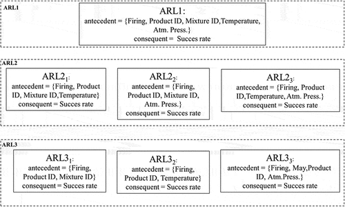
In the present case study, ARL1 is defined as the set of rules that describe the firing process with all five parameters (Machine ID, Product ID, Mixture ID, Avg ambient Temp. and Atm. Press) as antecedent and the success rate as consequent.

ARL2 is composed of three groups of ARs that have different combinations of variable parameters as antecedents:

• ARL2₁: have the Machine ID (firing process), Product ID, Mixture ID and Temperature as antecedent.

• ARL2₂: have as antecedent the type of process (firing process), Product ID, Mixture ID and Atm. Press.

• ARL2₃: have as antecedent the type of process (firing process), Product ID, Temperature, and Atm. Press.

In the same way, ARL3 have three groups of ARs too characterised in the following way:

• ARL3₁: have as antecedent the type of process (firing process), Product ID and Mixture ID.

• ARL3₂: have as antecedent the type of process (firing process), Product ID and Temperature.

• ARL3₃: have as antecedent the type of process (firing process), Product ID and Atm. Press.

For each level, the first step is to find the most frequent sets in the dataset. The minimum support and minimum confidence thresholds are set to min_support = 0,005 and min_confidence = 0,000. These two values are set relatively low to find all possible rules to identify the process.

To extract the ARs from the dataset, an application was developed based on the Mlxtend library (Raschka, 2018). The characteristics of the JOBs that must be scheduled (Table 6) are compared with the frequent itemsets of ARL1. Suppose in ALR1 there are one or more rules that have as antecedents the exact characteristics of a JOB to be scheduled. In that case, the support and confidence values are calculated for the relative couple of antecedents-consequents. If there is no match between the JOB to be scheduled and the results in ARL1, the activity will be compared with the itemsets of ARL2. If there are no matches between the antecedents of one group in ARL2 and the characteristics of the firing process that must be scheduled, a last comparison will be made on the results of ARL3. This is an iterative process that stops when a match is found. The case where no correlations are found indicates that the attribute of the JOB under consideration has no precedent in the company’s history. In that case, the production managers estimate the success rate according to their experience.

An example of ARs results for each level using the previous five parameters, or a combination of them, as antecedent and Success Rate as a consequent is shown in Table 8. A total of 578 rules were found, divided into 141 rules for ARL1 and 294 for ARL2 (in particular: 121 for ARL2₁, 110 for ARL2₂ and 63 for ARL2₃). For ARL3, 143 rules were founded (divided into 81 rules for ARL31, 36 for ARL32, and 26 for ARL3₃).

Table 8. Part of the results from each ARL.

ARs	Level	Antecedents	Consequent [Success Rate]	Support	Confidence
1	ARL1	Firing/Product 1/Cer 1/20°C/1023 mbar	80%	0,006369	1
2	ARL1	Firing/Product 4/Cer 1/17°C’/1012 mbar	100%	0,006369	1
3	ARL1	Firing/Product 5/Cer 3/17°C’/1013 mbar	0%	0,012739	0,666667
…	…	…	…	…	…
142	ARL21	Firing/Product 1/Cer 4/26°C	50%	0,006369427	0,5
143	ARL21	Firing/Product 5/Cer 3/22°C	67%	0,006369427	0,25
144	ARL21	Firing/Product 4/Cer 1/15°C	100%	0,006369427	0,5
…	…	…	…	…	…
263	ARL22	Firing/Product 1/Cer 4/1021 mbar	60%	0,006369	0,333333
264	ARL22	Firing/Product 2/Cer 2/1021 mbar	100%	0,012739	0,5
265	ARL22	Firing/Product 2/Cer 1/1015 mbar	100%	0,006369	1
…	…	…	…	…	…
373	ARL23	Firing/Product 2/22°C/1017 mbar	67%	0,025478	0,5
374	ARL23	Firing/Product 6/25°C/1025 mbar	83%	0,006369	0,333333
375	ARL23	Firing/Product 1/17°C/1010 mbar	100%	0,006369	0,333333
…	…	…	…	…	…
436	ARL31	Firing/Product 2/Cer 4	67%	0,022099	0,235294
437	ARL31	Firing/Product 2/Cer 2	83%	0,005525	0,058824
438	ARL31	Firing/Product 1/Cer 1	100%	0,022099	0,25
…	…	…	…	…	…
517	ARL32	Firing/Product 3/19°C	75%	0,016853933	0,05
518	ARL32	Firing/Product 4/27°C	80%	0,005617978	0,01724138
519	ARL32	Firing/Product 3/19°C	100%	0,04494382	0,28571429
…	…	…	…	…	…
553	ARL33	‘Firing/Product 1/1011 mbar	0%	0,089172	0,269231
554	ARL33	‘Firing/Product1/1019 mbar	100%	0,242038	0,730769
555	ARL33	‘Firing/Product 3/1027 mbar	100%	0,070064	0,423077
…	…	…	…	…	…
578	ARL33	‘Firing/Product 6/1009 mbar	100%	0,006369	0,5

For example, line 554 of Table 8 describes that the firing process on Product 1 with an atmospheric pressure of 1019 millibar has the support of 0,2420. That means that these pairs of events are present in 24,20% of all transactions in ARL3₃. Confidence can also be interpreted as an estimate of the conditional probability, so the probability of finding 100% as a consequent in transactions when antecedents are ‘Firing/Product1/1019 mbar’ equals 730,769%.

4.2.1. Corrective factor calculation

From AR results, it is possible to predict the success rate of a production order based on historical data. This information is important in the decision-making process because, according to this success rate, it might be better to produce a larger quantity to avoid interruptions in the production chain.

Once a correlation has been found between the JOBs to be scheduled and a set of rules, a corrective factor is calculated based on the confidence value and the value of the consequent. This correction factor specifies the additional quantities to be produced over the customer’s required parts.

According to this approach, the authors of this paper developed the following equation to calculate the additional number of scheduled parts to avoid an order stockout.

(8) ${\mathit{Additionaln}}^{\circ }\mathit{of}\mathit{pieces}\mathit{to}\mathit{be}\mathit{manufactured}=\sum _{\mathit{j}}{\mathit{n}}_{\mathit{i}}\mathbf{\ast }\left(1-\mathit{p}{\mathit{b}}_{\mathit{ij}}\right)\mathbf{\ast }\mathit{con}{\mathit{f}}_{\mathit{ij}}$(8)

The terms of the equation are:

• $n_i$ represents the units of product i to be realised (customer demand).

• $\mathit{p}{b}_{\mathit{ij}}$ represents the percentage of good parts (Success Rate) of product i in the rule j.

• $\left(1-\mathit{p}{b}_{\mathit{ij}}\right)$represents the rejection rate or bad parts associated with the product i in rule j.

• $\mathit{con}{f}_{\mathit{ij}}$ represents the confidence of the rule j: product i $\to$ Success Rate = $\mathit{p}{b}_{\mathit{ij}}$.

equation (8)(8) ${\mathit{Additionaln}}^{\circ }\mathit{of}\mathit{pieces}\mathit{to}\mathit{be}\mathit{manufactured}=\sum _{\mathit{j}}{\mathit{n}}_{\mathit{i}}\mathbf{\ast }\left(1-\mathit{p}{\mathit{b}}_{\mathit{ij}}\right)\mathbf{\ast }\mathit{con}{\mathit{f}}_{\mathit{ij}}$(8) calculates the correction factor that must be added to the theoretical demand of pieces to be manufactured. This correction factor is added to the customer demands to avoid under-dimensioning during production due to damaged items and to have more accurate scheduling. If the result is not an integer, it is rounded toward the higher integer value. The sequence of steps described can be applied to all operations to be programmed. equation (8)(8) ${\mathit{Additionaln}}^{\circ }\mathit{of}\mathit{pieces}\mathit{to}\mathit{be}\mathit{manufactured}=\sum _{\mathit{j}}{\mathit{n}}_{\mathit{i}}\mathbf{\ast }\left(1-\mathit{p}{\mathit{b}}_{\mathit{ij}}\right)\mathbf{\ast }\mathit{con}{\mathit{f}}_{\mathit{ij}}$(8) supports the decision maker in considering the need to increase production based on the probability of making nonconforming parts. This equation considers that the increased quantity results in 100% compliant parts. Although this assumption is not true in all cases, it allows for a trade-off between two conflicting elements: on the one hand, the need to avoid stock-outs, and on the other hand, the focus placed on any excess product. In any case, the rounding to the next higher integer provided in the formula means that one has an additional piece serving as a buffer.

By comparing the JOBs to be programmed (Table 6) with the different ARs (Table 8), the correction factors can be calculated.

For example, they consider the JOB in line 28 of Table 6 an Avg ambient Temp. = 20°C and Atm. Press = 1023 mbar, the Data Analytics phase associates Antecedents and the Consequent. The Analytics phase extracted the rules shown in Table 8. The two lines of Table 9 highlight two rules in ARL1 that describe the JOB present in line 28 of Table 6.

Table 9. Ars extracted for JOB 28 of Table 6.

Rules	#JOB in Table 6	ARs Level	Antecedent	Consequent	Confidence
1	28	ARL1	(‘Firing’, ‘Product 3’, ‘Cer 3’, ‘20°C’, ‘1023 mbar’)	40%	0,33
2	28	ARL1	(‘Firing’, ‘Product 3’, ‘Cer 3’, ‘20°C’, ‘1023 mbar’)	100%	0,67

The first line of Table 9 shows a probability equal to 33% (Confidence) to obtain a Success Rate equal to 40% when the Firing process is made on Product 3 with ceramic Cer3, 20°C as temperature and 1023 millibar as atmospheric pressure, while the second line says that there is a 67% probability that all pieces meet the quality requirements. Based on these data, it is possible to obtain the value of the corrective factor for Product 3 in these specific conditions of Material ID, Temperature, Atm. Press. by applying equation (8)(8) ${\mathit{Additionaln}}^{\circ }\mathit{of}\mathit{pieces}\mathit{to}\mathit{be}\mathit{manufactured}=\sum _{\mathit{j}}{\mathit{n}}_{\mathit{i}}\mathbf{\ast }\left(1-\mathit{p}{\mathit{b}}_{\mathit{ij}}\right)\mathbf{\ast }\mathit{con}{\mathit{f}}_{\mathit{ij}}$(8) :

$\left[10\ast \left(1-0,4\right)\ast 0.33\right]+\left[10\ast \left(1-1\right)\ast 0,67\right]=1.98+0=1.98\to 2$

In this case, equation (8)(8) ${\mathit{Additionaln}}^{\circ }\mathit{of}\mathit{pieces}\mathit{to}\mathit{be}\mathit{manufactured}=\sum _{\mathit{j}}{\mathit{n}}_{\mathit{i}}\mathbf{\ast }\left(1-\mathit{p}{\mathit{b}}_{\mathit{ij}}\right)\mathbf{\ast }\mathit{con}{\mathit{f}}_{\mathit{ij}}$(8) shows that it is better to plan two more pieces to avoid an order shortcoming.

4.3. Optimization, control and learning phase

The Optimization Model is applied to solve the FSSP present in this case study. Every machine is characterised by its matrix setup times that highlight the time necessary to pass from the production of an article to the next one. Product setup times on all workstations and the machines’ availability are considered through a connection with the PLM and Management System.

In this case study, the company aims to minimise the production program makespan, the total time required to complete all program tasks.

The algorithms developed to solve this problem are based on equations explained in section 3.1 and were realised in Python. Various optimisation features, supported by the open-source Python program, have been used. In particular, ‘gurobi’ was used as solver, and Pyomo library on Python 3.8.10 has been implemented into the mathematical problem.

The framework was tested for the case study on a computer with processor Intel 12th Gen Intel(R) Core (TM) i9-12900KF 3.20 GHz and 32 Gigabytes RAM. The results of all steps of the framework are provided in 1,25 seconds.

The optimisation model solution is shown in Table 10, with the relative Gantt chart shown in Figure 5 for a scheduling program comprising five products.

Figure 5. Job schedule’s Gantt chart and machine schedule’s Gantt chart.

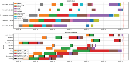
Table 10. Scheduling program.

JOB	Machine	Material	Start	Finish
(‘Product 3’, ‘Cer 3’)	Material tests	Cer 3	2 May 2022 06:00:00	2 May 2022 06:00:00
(‘Product 3’, ‘Cer 3’)	Casting	Cer 3	2 May 2022 06:00:00	2 May 2022 06:23:47
(‘Product 1’, ‘Cer 1’)	Material tests	Cer 1	2 May 2022 06:02:00	2 May 2022 06:29:00
(‘Product 3’, ‘Cer 3’)	Demoulding	Cer 3	2 May 2022 06:23:48	2 May 2022 06:51:48
(‘Product 1’, ‘Cer 1’)	Casting	Cer 1	2 May 2022 06:29:00	2 May 2022 07:17:00
(‘Product 2’, ‘Cer 2’)	Material tests	Cer 2	2 May 2022 06:31:00	2 May 2022 07:31:00
…	…	…	…	…

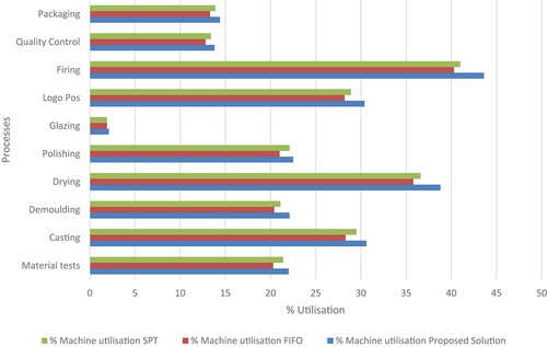
The proposed solution was compared with two traditional heuristics algorithms: First-In-First-Out (FIFO) logic and Short Processing Time (SPT) logic. The FIFO logic schedules JOBS according to the order in which they arrive; the first order that arrives will be the first to be processed. On the other hand, SPT logic schedules JOBS according to the shortest processing time, so the tasks with the shortest processing time will be the first to be scheduled. The proposed method improves the makespan value by 9% compared to the FIFO strategy and by 6% compared to the latter. Figure 6 shows the percentage of utilisation of the machines for each process. The proposed solution improves production efficiency by reducing unproductive machine times.

Figure 6. Percentage of machine utilisation for the proposed solution, FIFO and SPT strategies.

After the optimisation phase, the scheduling plan will be provided to the operation managers to be executed. The optimisation phase is data-driven and receives information from the MES in near-real time mode. This means, for example, that if we have planned to have a corrective factor of 10 pieces for product X. Still, during the firing of the pieces, 15 pieces are found to be discarded, the optimisation program will be relaunched to re-schedule the JOBs taking into consideration the five extra discarded pieces (15–10). Usually, the company relaunches the optimisation program 3 to 6 times a day.

Moreover, during the production control phase, a comparison will be carried out between real and predicted Success Rates for every product order. Real data are collected on the shop floor using company MES to identify corrective factors to be introduced for the following scheduling plans, according to a self-learning approach. It is of interest to be able to appropriately define time intervals for updating the database. In this way, it will also be possible to determine when it is appropriate to update the new ARs. Since these are data-driven processes, the results of the analyses must be up to date and ready to be used to adapt production as promptly as possible. Given that the state of the art defines no time interval, it makes sense to propose at least one day between successive updates. This allows the company to assimilate the new suggestions provided by the data-driven analysis and, simultaneously, does not leave too wide an interval that would compromise the results’ validity.

5. Discussions

Thousands of complex rules to operationalise are often the result of association rule mining. Furthermore, different approaches frequently produce different results, and it is challenging to choose the method and the associated parameters that are most appropriate for the data at hand without thoroughly comprehending the underlying statistical concepts on the user’s part. In particular, methodologies, such as regression models, are ineffective without well-defined hypotheses and a thorough comprehension of the data collection procedure (Genga et al., 2022). The methodology exemplified in this research aims to work around this issue, providing a self-learning framework capable of collecting and analysing production data to generate scheduling plans more relevant to the industry context.

5.1. Theoretical contributions

It is crucial to determine and control the probability, consequences, and any variables that could impact the program to maximise the likelihood of developing an accurate production scheduling program. Creating a mechanism for merging complex data sets from various sources is one of the challenges faced during this research. In the case study presented in this work, data came with diverse velocities and originated from multiple sources affected by veracity issues. To support the manufacturing company’s decision-making process, an N-dimensional analysis of environmental performance data must be performed using the data sets and data streams gathered from wired and wireless sensors and meters. The proposed dataset includes data archival, but business managers require help sifting through the vast amount of collected data to find the necessary information. This work addresses this gap by creating a framework that can be used to combine and analyse complex data sets using a Big Data Analytics approach. Massive, varied, and regularly produced data collections present a considerable management challenge due to the complexity and volatility of the datasets and the development in their amount, making processing and analysis highly challenging. Since the variables in our case study offered certain crucial elements, the inherent structure and complexity of the data obtained can render it unsafe to utilise conventional tools for analysis. First, there are a lot of potential predictors. For general typical statistical research, this is rather challenging. The independence hypothesis is commonly adopted in a parametric analysis, but the relationship between the independent variables may present problems in this study. At last, the distribution of the data showed non-homogeneity and non-linearity. This paper indicates that Association Rules are an effective alternative to the conventional parametric procedures often used in production scheduling problems. To define ‘all’ potential links among factors and causes affecting the production program, association rules, in particular, appear suited for analysis of the production schedule parameters. When the production process is characterised by constant antecedents (attributes that the company continuously records) and variable antecedents (attributes that may change from one machining operation to the next), the algorithm proposed in section 3.2 allows the company managers to evaluate a consequence.

Even the essential support and confidence levels set to influence the association rules extracted. A threshold greater than 0 can imply the loss of some rules, specifically those with a low probability of occurrence. This parameter’s importance increases with the dataset’s size because the number of Association Rules to be mined influences how quickly the algorithm runs.

5.2. Practical implications

The definition of a strategy that permits a logical and automatically feasible approach to production scheduling can significantly enhance the way work is organised and decision-making processes are conducted. Traditional production optimisation models do not predict the defective parts generated during production processes and, therefore, do not consider the actual quantities to be produced in order not to have stockouts or rework. Thus, a company should have a programme to minimise the makespan without considering that the final quantities produced were lower than those required by customers due to quality defects created during the production processes.

The proposed framework makes it possible to predict the number of defective parts that will be created and thus gives the optimisation model the correct quantity values to produce.

The ability to predict errors during one or more stages of the production process is of fundamental importance, especially in decision-making processes supporting the production planner. The proposed framework assists the production planner in two basic steps: risk analysis in the production process and scheduling production orders using a mathematical approach.

The mathematical model guarantees the search for the global optimum solution to the optimisation problem, which in the case study is to minimise the makespan. Finding the optimal production sequence for a given objective function ensures greater efficiency in using available resources, avoiding long, unproductive times. Therefore, this approach guarantees a higher level of goodness in the solution, better than traditional FIFO and SPT logics, in reduced calculation times. The latter aspect is crucial because it allows the generation of several scheduling plans per day based on possible problems at the production site, such as machine breakdowns, lack of resources, etc. This approach increases the possibility of delivering a production batch on time and avoiding delays caused by non-conformities during the production process.

The novel integration of the Association Rule Mining and mathematical models within the same data-driven framework represents a promising approach to managing scheduling problems.

Additionally, it depends on data-driven analysis: things are not clustered based on their category but rather by considering past data. In this way, not only will reliable production quantity be predicted, but a further knowledge dimension will be added since previously unknown patterns are derived through Association Rule Mining. Additionally, this method avoids developing a research hypothesis for a factor combination, which can be time- and resource-intensive even for a collection with a reasonable number of variables (Fani et al., 2023).

Some issues relating to human behaviour have been seen while the recommended study approach has been implemented in the ceramics firm. Various data must be considered to use the built data-driven decision support system. Securing data recording correctness and standardising them to prevent duplications is one of the primary criticisms in this regard. The various data sources were initially used separately and not merged in the case study suggested in this paper. Standardised processes are required to address this problem since they will help operators record the appropriate data correctly and prevent errors and forgetfulness in the data management process. A significant cultural shift is required to instil in all employees the idea that precise data collecting and recording is the first step toward developing a successful data-driven decision support system and accurately forecasting the scheduling activities.

6. Conclusions

This paper exemplifies a self-learning framework for collecting and processing industrial data integrated with a mathematical model for solving scheduling problems in an unstable production environment. In this way, ARs are used to extract features or correlations from vast amounts of data to make the scheduling plan more reliable. The framework was tested in a real industrial scenario in the ceramic manufacturing sector. The case study presented in this paper examines the firing process of several products manufactured by the company. These items can be made from different types of ceramics, each producing different results in the analysed process. This study presents a framework capable of predicting possible irregularities in the production process. It proposes a correction factor for production quantities to avoid the need for urgent rework, which would result in a longer time-to-market.

The corrective factor offers increased production quantities based on historical data related to a process with certain conditions. In this way, a slightly higher number will be produced than required so that the delivery time can be met more accurately by predicting a percentage of defects in the workmanship.

The proposed framework is part of a self-learning cycle. The data used for scheduling will have to be produced in a given time frame. The results of the production process will, in turn, be integrated into the dataset, thus enriching the information content from which ARs can be extracted. In this way, the accuracy of the results of the ARs, and consequently of the entire framework, will be improved as there will be more and more data on which to estimate rules describing the firing process. It will also be possible to increase the threshold levels for support and confidence to extract only the events (antecedent and consequent) that occur most often.

6.1. Limitations and future research

The main limitation of the presented work regards the information in the given dataset for the case study. In particular, for the Data Analytic Phase, information such as the electrical power absorption of the oven is missing. The mathematical problem also does not consider the availability of the raw materials, semi-finished products in stock and operators needed for the production phase. This valuable information can help the company’s decision-making processes better understand the quantities that can be produced. To generalise the framework to consider different types of production environments, future developments could include having several machines in parallel for the same task. This would include scheduling problems such as Flexible JSSP or Flexible FSSP in the framework. On the other hand, the increase in complexity in the mathematical model could lead to a considerable increase in the calculation time of the framework. The problem of high computation times for large and complex instances has led researchers in various fields to approach the problem using hybrid algorithms, meta-heuristic algorithms, hyper-heuristic algorithms, adaptive algorithms, island algorithms, polyploid algorithms, memetic algorithms, etc (M. Chen & Tan, 2023; Dulebenets, 2023; Singh et al., 2022). Thus, the following steps will also compare the approaches to solving the problem presented in the framework. In this way, it will be possible to compare the impact of advanced optimisation algorithms, such as those mentioned above, and machine learning approaches, such as RL versus mathematical models (Dulebenets, 2021). This comparison will provide a better understanding of each methodology’s potential advantages and limitations in the specific context of the problem addressed.

Acknowledgement

We are very grateful for the support of the European Union’s Horizon Europe research and innovation programme, under grant agreement No. 101057294, AIDEAS (AI-Driven industrial Equipment) project.

Disclosure statement

No potential conflict of interest was reported by the author(s).

Additional information

Funding

This work was supported by the European Commission [101057294].

References

- Agrawal, R., & Srikant, R. (1994). Fast algorithms for mining association rules. Proceedings 20th International Conference Massive Data Bases, VLDB, Santiago, Chile (pp. 1215).
- Al-Banna, A., Rana, Z. A., Yaqot, M., & Menezes, B. C. (2023). Supply chain resilience, industry 4.0, and investment interplays: A review. Production & Manufacturing Research, 11(1), 2227881. https://doi.org/10.1080/21693277.2023.2227881
- Antomarioni, S., Ciarapica, F. E., & Bevilacqua, M. (2022). Association rules and social network analysis for supporting failure mode effects and criticality analysis: Framework development and insights from an onshore platform. Safety Science, 150, 105711. https://doi.org/10.1016/j.ssci.2022.105711
- Azab, E., Nafea, M., Shihata, L. A., & Mashaly, M. (2021). A machine-learning-assisted simulation approach for incorporating predictive maintenance in dynamic flow-shop scheduling. Applied Sciences (Switzerland), 11(24), 11725. https://doi.org/10.3390/app112411725
- Babor, M., Paquet-Durand, O., Kohlus, R., & Hitzmann, B. (2023). Modeling and optimization of bakery production scheduling to minimize makespan and oven idle time. Scientific Reports, 13(1). https://doi.org/10.1038/s41598-022-26866-9
- Bala, P. K., Sural, S., & Banerjee, R. N. (2010). Association rule for purchase dependence in multi-item inventory. Production Planning & Control, 21(3), 274–28. https://doi.org/10.1080/09537280903326578
- BCI Supply Chain Resilience Report. (2023). Retrieved January, 2024. https://www.thebci.org/resource/bci-supply-chain-resilience-report-2023.html
- Chen, Y. (2019). Research on resource allocation optimization of information management system based on big data association mining. Journal of Physics: Conference Series, 1345(2), 022073. https://doi.org/10.1088/1742-6596/1345/2/022073
- Chen, M., & Tan, Y. (2023). SF-FWA: A self-adaptive fast fireworks algorithm for effective large-scale optimization. Swarm and Evolutionary Computation, 80, 101314. https://doi.org/10.1016/j.swevo.2023.101314
- Crespo Márquez, A., de la Fuente Carmona, A., & Antomarioni, S. (2019). A process to implement an artificial neural network and association rules techniques to improve asset performance and energy efficiency. Energies, 12(18), 3454. https://doi.org/10.3390/en12183454
- Del Gallo, M., Mazzuto, G., Ciarapica, F. E., & Bevilacqua, M. (2023). Artificial intelligence to solve production scheduling problems in real industrial settings: Systematic literature review. Electronics, 12(23), 4732. https://doi.org/10.3390/electronics12234732
- Dulebenets, M. A. (2021). An adaptive polyploid memetic algorithm for scheduling trucks at a cross-docking terminal. Information Sciences, 565, 390–421. https://doi.org/10.1016/j.ins.2021.02.039
- Dulebenets, M. A. (2023). A diffused memetic optimizer for reactive berth allocation and scheduling at marine container terminals in response to disruptions. Swarm and Evolutionary Computation, 80, 101334. https://doi.org/10.1016/j.swevo.2023.101334
- Fani, V., Antomarioni, S., Bandinelli, R., & Bevilacqua, M. (2023). Data-driven decision support tool for production planning: A framework combining association rules and simulation. Computers in Industry, 144, 103800. https://doi.org/10.1016/j.compind.2022.103800
- Genga, L., Allodi, L., & Zannone, N. (2022). Association rule mining meets regression analysis: An automated approach to unveil systematic biases in decision-making processes. Journal of Cybersecurity and Privacy, 2(1), 191–219.
- Habib Zahmani, M., & Atmani, B. (2021). Multiple dispatching rules allocation in real-time using data mining, genetic algorithms, and simulation. Journal of Scheduling, 24(2), 175–196. https://doi.org/10.1007/s10951-020-00664-5
- Jacso, A., Szalay, T., Sikarwar, B. S., Phanden, R. K., Singh, R. K., & Ramkumar, J. (2023). Investing conventional and ANN-based feed rate scheduling methods in trochoidal milling with cutting force and acceleration constraints. International Journal of Advanced Manufacturing Technology, 127(1–2), 487–506. https://doi.org/10.1007/s00170-023-11506-x
- Jing, X., Yao, X., Liu, M., & Zhou, J. (2022). Multi-agent reinforcement learning based on graph convolutional network for flexible job shop scheduling. Journal of Intelligent Manufacturing, 35(1), 75–93. https://doi.org/10.1007/s10845-022-02037-5
- Marcucci, G., Ciarapica, F. E., Mazzuto, G., & Bevilacqua, M. (2023). Analysis of ripple effect and its impact on supply chain resilience: A general framework and a case study on agri-food supply chain during the COVID-19 pandemic. Operations Management Research, 17(1), 175–200. https://doi.org/10.1007/s12063-023-00415-7
- Marcucci, G., Mazzuto, G., Bevilacqua, M., Ciarapica, F. E., & Urciuoli, L. (2022). Conceptual model for breaking ripple effect and cycles within supply chain resilience. Supply Chain Forum: An International Journal, 23(3), 252–271. https://doi.org/10.1080/16258312.2022.2031275
- Nasiri, M. M., Salesi, S., Rahbari, A., Salmanzadeh Meydani, N., & Abdollai, M. (2019). A data mining approach for population-based methods to solve the JSSP. Soft Computing, 23(21), 11107–11122. https://doi.org/10.1007/s00500-018-3663-2
- Parameshwaran Pillai, T., & Vijayan, S. (2022). Application of machine learning algorithm in a multi-stage production system. Transactions of Famena 46(1), 91–102. https://doi.org/10.21278/tof.461033121fatcat:6lsj64kz4vds7oafon4hixmzmq
- Qiu, Y., Sawhney, R., Zhang, C., Chen, S., Zhang, T., Lisar, V. G., Jiang, K., & Ji, W. (2019). Data mining–based disturbances prediction for job shop scheduling. Advances in Mechanical Engineering, 11(3), 168781401983817. https://doi.org/10.1177/1687814019838178
- Raschka, S. (2018). Mlxtend: Providing machine learning and data science utilities and extensions to python’s scientific computing stack. Journal of Open Source Software, 3(24), 638. https://doi.org/10.21105/joss.00638
- Said, N. E. D. A., Samaha, Y., Azab, E., Shihata, L. A., & Mashaly, M. (2021). An online reinforcement learning approach for solving the dynamic flexible job-shop scheduling problem for multiple products and constraints. In Proceedings - 2021 International Conference on Computational Science and Computational Intelligence, CSCI 2021, 134–139. https://doi.org/10.1109/CSCI54926.2021.00095.
- Salimbeni, S., Redchuk, A., & Rousserie, H. (2023). Quality 4.0: Technologies and readiness factors in the entire value flow life cycle. Production & Manufacturing Research, 11(1), 2238797. https://doi.org/10.1080/21693277.2023.2238797
- Sanchis, R., Marcucci, G., Alarcón, F., & Poler, R. (2021). Knowledge registration module design for enterprise resilience enhancement. IFAC-Papersonline, 54(1), 1029–1034. https://doi.org/10.1016/j.ifacol.2021.08.122
- Serrano-Ruiz, J. C., Mula, J., & Poler, R. (2021). Smart manufacturing scheduling: A literature review. Journal of Manufacturing Systems, 61, 265–287. https://doi.org/10.1016/j.jmsy.2021.09.011
- Singh, P., Pasha, J., Moses, R., Sobanjo, J., Ozguven, E. E., & Dulebenets, M. A. (2022). Development of exact and heuristic optimization methods for safety improvement projects at level crossings under conflicting objectives. Reliability Engineering & System Safety, 220, 108296. https://doi.org/10.1016/j.ress.2021.108296
- Subramaniyan, M., Skoogh, A., Salomonsson, H., Bangalore, P., Gopalakrishnan, M., & Muhammad, A. S. (2018). Data-driven algorithm for throughput bottleneck analysis of production systems. Production & Manufacturing Research, 6(1), 225–246. https://doi.org/10.1080/21693277.2018.1496491
- Troncoso-García, A. R., Martínez-Ballesteros, M., Martínez-Álvarez, F., & Troncoso, A. (2023). A new approach based on association rules to add explainability to time series forecasting models. Information Fusion, 94, 169–180. https://doi.org/10.1016/j.inffus.2023.01.021
- Wang, L., Lin, B., Chen, R., & Lu, K. H. (2022a). Using data mining methods to develop manufacturing production rule in IoT environment. The Journal of Supercomputing, 78(3), 4526–4549. https://doi.org/10.1007/s11227-021-04034-6
- Wang, X., Zhang, L., Lin, T., Zhao, C., Wang, K., & Chen, Z. (2022b). Solving job scheduling problems in a resource preemption environment with multi-agent reinforcement learning. Robotics and Computer-Integrated Manufacturing, 77, 102324. https://doi.org/10.1016/j.rcim.2022.102324
- Yang, L., Zhang, F., Liu, A., Zhou, S., Wu, X., Wei, F., Yang, L., Zhang, F., Liu, A., Zhou, S., Wu, X., and Wei, F. (2022). A study on the identification of delayed delivery risk transmission paths in multi-variety and low-volume enterprises based on bayesian network. Applied Sciences, 12(23), 12024. https://doi.org/10.3390/APP122312024
- Zafarzadeh, M., Wiktorsson, M., & Baalsrud Hauge, J. (2023). Capturing value through data-driven internal logistics: Case studies on enhancing managerial capacity. Production & Manufacturing Research, 11(1), 2214799. https://doi.org/10.1080/21693277.2023.2214799
- Zhang, H. N., & Dwivedi, A. D. (2022). Precise marketing data mining method of E-Commerce platform based on association rules. Mobile Networks & Applications, 27(6), 2400–2408. https://doi.org/10.1007/s11036-021-01886-3
- Zhang, Y., Zhu, H., Tang, D., Zhou, T., & Gui, Y. (2022). Dynamic job shop scheduling based on deep reinforcement learning for multi-agent manufacturing systems. Robotics and Computer-Integrated Manufacturing, 78, 102412. https://doi.org/10.1016/j.rcim.2022.102412
- Zhao, A., Liu, P., Gao, X., Huang, G., Yang, X., Ma, Y., Xie, Z., & Li, Y. (2022). Data-mining-based real-time optimization of the job shop scheduling problem. Mathematics, 10(23), 4608. https://doi.org/10.3390/math10234608
- Zhou, T., Tang, D., Zhu, H., & Zhang, Z. (2021). Multi-agent reinforcement learning for online scheduling in smart factories. Robotics and Computer-Integrated Manufacturing, 72, 102202. https://doi.org/10.1016/J.RCIM.2021.102202
- Zhou, L., Zhang, L., Ren, L., & Wang, J. (2019). Real-time scheduling of cloud manufacturing services based on dynamic data-driven simulation. IEEE Transactions on Industrial Informatics, 15(9), 5042–5051. https://doi.org/10.1109/tii.2019.2894111