Spectral–spatial feature extraction using orthogonal linear discriminant analysis for classification of hyperspectral data

ABSTRACT

Hyperspectral image classification is among the most frequent topics of research in recent publications. This paper proposes a new supervised linear feature extraction method for classification of hyperspectral images using orthogonal linear discriminant analysis in both spatial and spectral domains. In fact, an orthogonal filter set and a spectral data transformation are designed simultaneously by maximizing the class separability. The important characteristic of the presented approach is that the proposed filter set is supervised and considers the class separability when extracting the features, thus it is more appropriate for feature extraction compared with other filters such as Gabor. In order to compare the proposed method with some existing methods, the extracted spatial–spectral features are fed into a support vector machine classifier. Some experiments on the widely used hyperspectral images, namely Indian Pines, Pavia University, and Salinas data sets, reveal that the proposed approach leads to state-of-the-art performance when compared to other recent approaches.

KEYWORDS:

• Classification
• linear discriminant analysis
• orthogonal linear discriminant analysis
• spatial features
• spectral information
• hyperspectral imaging
• support vector machine

Introduction

The availability of remotely sensed hyperspectral images acquired in the adjacent bands of the electromagnetic spectrum, makes it necessary to propose techniques by which one is able to interpret such high-dimensional data in various applications (Aguilar, Fernández, Aguilar, Bianconi, & Lorca, 2016 Nagabhatla & Kühle, 2016; Plaza et al., 2009; Zehtabian & Ghassemian, 2016). One of the most important applications of hyperspectral images is classification in which land covers are distinguished from each other. For this purpose, several techniques have been developed using the rich source of spectral information along with spatial information buried in the hyperspectral images (Su, 2016).

Various experiments have proven the sparseness of high-dimensional data spaces such that the data structure involved exists primarily in a subspace (Green et al., 1998). As a consequence, there is a need for feature extraction methods by which the dimensionality of the data can be reduced to the right subspace without losing the essential information that allows for the separation of classes. These techniques can be mainly classified into two categories (Li et al., 2015). (1) Several methods use the linear transforms to extract the spectral or spatial information from hyperspectral data. Widely used linear feature extraction methods in the spectral domain include the principal component analysis (PCA) (Plaza, Martinez, Plaza, & Perez, 2005), independent component analysis (ICA) (Bayliss, Gualtieri, & Cromp, 1997), and linear discriminant analysis (LDA) (Bandos et al., 2009), while those in the spatial domain include Gabor filter bank (Mirzapour & Ghassemian, 2015) and wavelets. (2) Several techniques exploit spectral or spatial features obtained through nonlinear transformations. Examples of these methods are morphological analysis (Benediktsson, Palmason, & Sveinsson, 2005; Plaza et al., 2005), kernel methods (Camps-Valls & Bruzzone, 2005), and manifold regularization (Ma, Crawford, & Tian, 2010).

On the other hand, feature extraction methods can be classified into either supervised or unsupervised ones. For instance, PCA, Gabor filter bank, ICA, and morphological analysis are unsupervised, i.e. these methods do not use the training samples available for the classification procedure. But, LDA is an example of supervised methods whose features are extracted by considering training samples. Some state-of-the-art supervised methods are: (1) Partlets-based methods which use a library of pretrained part detectors (Cheng et al., 2015). (2) kernel-based feature selection which maximizes the separability of the feature space with respect to the radial basis function (RBF) kernel (Kuo, Ho, Li, Hung, & Taur, 2014). (3) rotation-invariant and fisher discriminative convolutional neural networks which introduces and learns a rotation-invariant layer and a Fisher discriminative layer, respectively, on the basis of the existing high-capacity CNN architectures (Cheng, Zhou, & Han, 2016). (4) collection of part detectors which uses a set of part detectors to detect objects or spatial patterns within a certain range of orientation (Cheng, Han, Zhou, & Guo, 2014).

This paper focuses on using linear transformations for feature extraction and feature reduction. Linear transformations are attractive for image processing owing to the fact that they have a very low computational burden, while at the same time they are successful in extracting relevant information from hyperspectral images.

To linearly extract the spectral and spatial features, a possible solution is LDA, which not only has an easy implementation but also has a clear physical interpretation. In addition, it provides high classification accuracy. These good capabilities make it very useful in practical applications such as hyperspectral feature extraction. However, LDA has not been yet used to design a filter able to extract the spatial features of hyperspectral imagery. Therefore, this paper proposes a new orthogonal LDA-based filter set extracting the spatial features of hyperspectral data and maximizing the class separability.

In spite of the fact that LDA provides good performance, conventional LDA cannot work in ill-posed problems, when the number of training samples is less than the number of features (Bandos et al., 2009). To overcome the singularity problem, many approaches have been proposed, including uncorrelated LDA (ULDA), orthogonal linear discriminant analysis (OLDA), regularized LDA (RLDA), etc. (Bandos et al., 2009; Ye & Xiong, 2006a).

The transformation used in the OLDA method is based on the simultaneous diagonalization of both between-class and within-class scatter matrices, by which the singularity problem is solved implicitly (Ye & Xiong, 2006a). On the other hand, the performance of OLDA is better than that of ULDA (Ye, 2005). This is due to the effect of the noise removal property inherent in OLDA (Ye, 2005). In addition, because OLDA does not search over the regularization parameter, the computational burden of it is very low in comparison with that of RLDA (Bandos et al., 2009). Therefore, OLDA is an appropriate feature extraction method.

One of the main disadvantages of LDA-based methods, particularly when used for extracting spatial features, is that the number of LDA features is equal to the number of classes minus one. Due to this limitation, the sufficient number of features cannot be extracted. For example, in the Pavia University data, there are only nine classes of materials. So, only eight features can be extracted by LDA-based methods. These features do not contain the essential information that allows for the separation of classes. To cope with this problem, we have used the solution proposed in Okada and Tomita (1985). We will describe the solution in the corresponding section of the paper.

The paper is structured in seven sections. Section 2 presents the LDA and OLDA feature reduction methods. Extracting the spatial features based on OLDA and PCA is proposed in Section 3. The proposed methodology is presented in Section 4. In Section 5, the support vector machine (SVM) classifier is reviewed. Section 6 is devoted to the experimental results and discussions. Eventually, our conclusions are given in Section 7.

Linear discriminant analysis and orthogonal linear discriminant analysis

The following subsections review the classical LDA and OLDA as presented in Bandos et al. (2009), Ye and Xiong (2006a).

Linear discriminant analysis

Given a data matrix , where each column corresponds to a training sample and each row corresponds to a particular feature, we consider finding a linear transformation matrix G that maps each column (1in) of in the m-dimensional space to a vector in the l-dimensional space, i.e. (l < m).

In classical LDA, the transformation matrix G is computed so that low-dimensional feature space fulfills a given maximization criterion of separability among class distributions:

(1)

where is the between-class scatter matrix, is the within-class scatter matrix, and , and are the mean vectors of class k, the index set, and the number of training samples of class k, respectively. In addition, is the mean vector of the data, K is the number of classes, and n is the number of training samples. The maximization criterion in Equation (1) can be rewritten as the following maximization problem:

(2)

where denotes the estimate of the covariance matrix. It is worth mentioning that the solution of Equations (1) and (2) can be obtained if and are nonsingular. The scatter matrices , and can be redefined as:

(3)

where

(4)

(5)

(6)

in which O is a column vector of n ones, is a column vector of ones, and denotes the data matrix of elements in class k. Note that matrices and are singular when the number of observations is smaller than the number of features, and consequently, the solution cannot be obtained. The OLDA method, described in the following subsection, can alleviate this problem.

Orthogonal linear discriminant analysis

OLDA has been proposed by Ye, et al. as an extended version of classical LDA (Ye, 2005). Unlike LDA, OLDA provides orthogonal features. In addition, OLDA can be used even if all scatter matrices are singular, and as a consequence, it solves the singularity problem to some extent. The OLDA algorithm can be decomposed into three steps (Ye & Xiong, 2006b): (1) removing the null-space of the estimated covariance matrix ; (2) using classical ULDA as an intermediate step; and (3) applying an orthogonalization step to the output of the ULDA transformation. The optimal transformation in OLDA is obtained by solving the following optimization problem:

(7)

where † denotes pseudo-inverse. On the one hand, the pseudo-inverse of a matrix is well defined, when the inverse of a matrix does not exist. On the other hand, pseudo-inverse of a matrix coincides with its inverse, when the matrix is invertible. The orthogonality condition is then imposed on the constraint (step 3 of the algorithm). The main advantage of OLDA is that it is less susceptible to overfitting and more robust against noise than other LDA-based methods e.g. ULDA (Ye, 2005). The overfitting phenomenon generally occurs when a model is excessively complex, such that there are too many parameters relative to the number of training samples. Thus, to work well, when the number of training samples is limited, the proposed method uses OLDA for feature extraction. In summary, we prefer OLDA for the following reasons: (1) the performance of OLDA is better than that of ULDA (Ye, 2005); (2) overfitting is not a serious problem in OLDA; (3) the computational burden of OLDA is less than that of RLDA; (4) the eigenvectors of OLDA are orthogonal to each other which are in harmony with the Gram–Schmidt procedure used in our methodology (see Sections 3 and 4), such that all of the extracted features are orthogonal to each other (see Okada and Tomita (1985), Ye, Janarda, Li, and Park (2006), Ye and Xiong (2006b) for more details).

Designing a filter bank based on OLDA and PCA

This section proposes a new filter bank which is able to extract the spatial information of a single band image. The proposed filer bank aims at maximizing the Fisher score.

Let the single band image be denoted by , where r₁ and r₂ are the number of rows and columns in the image, respectively, and the two-dimensional (2-D) kernel be denoted by h:

(8)

To extract the spatial information of the image I, we should obtain A = I*h, where * denotes the convolution operation and the matrix A represents the extracted features. To obtain A(i, j), i.e. the (i, j)th element of matrix A, one should perform the following steps. Firstly, we rotate the matrix h 180° about its center. Secondly, we slide the center of the rotated kernel so that it lies on the (i, j)th element of I (see Figure 1). Finally, we multiply each element of the rotated kernel by the corresponding element of I and sum these values (see Figure 1). The convolution operation can also be represented by matrix multiplication. To obtain A(i, j), the element I(i, j) and its neighboring elements are inserted into a vector denoted by . In addition, the elements of the rotated kernel are inserted into a vector denoted by . Multiplying by gives A(i, j). This procedure is also shown at the bottom of Figure 1 (f is equal to 3 in this figure).

Figure 1. Performing convolution by matrix multiplication (f is set to 3 in this figure).

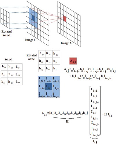
In fact, represents the initial feature space of the (i, j)th element of I and the kernel vector aims at extracting the relevant feature from the initial feature space . To obtain all of the elements of the matrix A, one should multiply the kernel vector by the matrix M representing the initial feature space of all of the pixels ():

(9)

Each column of M represents the initial feature space of the corresponding pixel. Using the matrix M, one can easily obtain the elements of the matrix A:

(10)

To use LDA-based methods, the data matrix should be formed, where each column corresponds to a training sample and each row corresponds to a particular feature (see Section 2. A). So, the new matrix V is defined representing the initial feature space of only training samples:

(11)

and

(12)

In fact, matrix V is the data matrix to which one can apply LDA-based methods and the kernel vector is the linear transformation which is denoted by G in the previous section. From these equations, one can see that the data matrix V is available and the kernel vector maximizing the Fisher score should be obtained. So, the kernel vector is equal to the eigenvector obtained by applying OLDA to the matrix V. Note that the 2-D kernel h can be easily obtained from the vector , because is a row-wise version of h (see Figure 1).

As mentioned in Section 1, the number of eigenvectors in LDA-based methods is equal to the number of classes minus one (K−1). So, a filter bank with K−1 kernels is formed in which the kernels are orthogonal to each other. Using this filter bank, one can extract K−1 features. However, the number of features (i.e. K−1) is not sufficient for the classification purpose, because essential information that allows for the separation of classes may be lost. To tackle this problem, the technique proposed in Okada and Tomita (1985) is used in which and are projected onto a subspace orthogonal to the computed eigenvectors, and the OLDA analysis is repeated in this subspace. So, after designing a number of filters (i.e. K−1) by the OLDA method, the matrices and are projected onto the subspace orthogonal to the space of the designed filters. Then, a new set of filters is designed. This process is iterated until the sufficient number of features is provided. The Gram–Schmidt method is employed in the process by which the orthogonal subspace is determined (Okada & Tomita, 1985). Note that the maximum number of orthogonal filters which can be designed is (because the dimension of H is ), and consequently, the maximum number of features for each pixel is .

Besides, one can extract the spatial features of a single band image by the PCA transform. To this end, we should apply PCA to the matrix M containing initial feature space of all of the samples. Note that PCA is an unsupervised method. So, we should consider all of the samples and that is why we do not apply the PCA to the matrix V. The principal components corresponding to most of the cumulative variance are the spatial features extracted by PCA. This technique is called spatial PCA (SPCA) by which one can extract the spatial features of a single band image in an unsupervised manner. If the PCA transform is used for extracting the spatial features, the set of orthogonal filters H is equal to eigenvectors of this transform.

Proposed methodology

The methods proposed in the previous section are efficient for extracting the spatial features of a single band image. Because hyperspectral sensors provide a large number of spectral bands, a feature extraction method should be able to extract spatial and spectral features from these images.

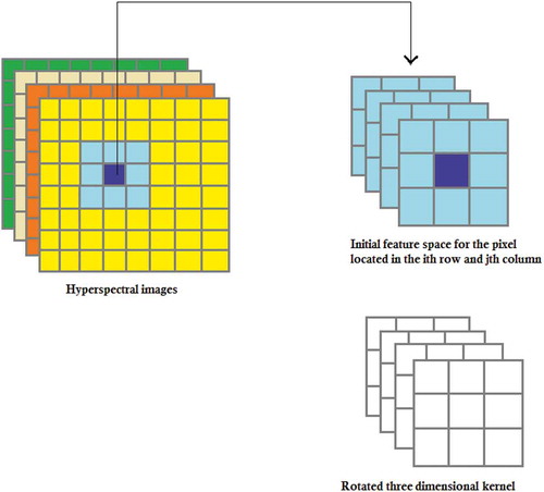
When hyperspectral images are used, the initial feature space of (i, j)th pixel is composed of not only the neighboring pixels in the spatial domain but also neighboring pixels in the spectral domain (see Figure 2). So, one should use a 3-D kernel to extract the relevant features (see Figure 2). Similar to the previous section, the kernel vector H is the row-wise version of the rotated 3-D kernel, the vector represents the initial feature space of the element (i, j), the matrix represents the initial feature space of all samples, and the matrix represents the initial feature space of training samples, where N is the number of spectral bands. In addition, multiplying H by V yields A, i.e. training samples. However, estimating the coefficients of the kernel by the reasonable number of training samples is not usually tractable (if OLDA is applied to the matrix V, overfitting occurs). For example, the Indian Pines data set has N = 200 spectral bands. If the length of the kernel f is set to 30, it is essential to estimate 200 × 30 × 30 = 180000 coefficients of the kernel vector H. Therefore, an initial dimensionality reduction stage such as PCA should be used to reduce the dimensionality of V. Using PCA along with an LDA-based method is a popular framework used to extract features from high-dimensional data (Yang & Yang., 2003).

Figure 2. Neighboring pixels for 3-D hyperspectral images (in this figure, f and N are set to 3 and 4, respectively).

To reduce the dimensionality of the matrix V, it should be multiplied by the eigenvectors obtained from applying PCA to M (because PCA is unsupervised, it should be applied to M). However, applying the PCA transform to the matrix is not possible, because of the high dimensionality of this matrix. On the one hand, using PCA in high-dimensional matrices is computationally expensive. On the other hand, to accurately estimate the coefficients of PCA, the value of should be large enough in comparison to (to accurately estimate the covariance matrix of PCA, the number of samples should be several times larger than that of dimension/features). The latter condition is not necessarily satisfied by the matrix M. So, the proposed strategy is as follows:

1. Apply the PCA transform to the spectral bands of hyperspectral data and retain the principal components corresponding to 90% of the cumulative variance. This stage reduces the dimension of spectral bands to few principal components. In fact, this step extracts the spectral information of the hyperspectral data. Suppose that the number of retained principal components is Nu, where Nu ≪ N (see Figure 3).

2. Apply the SPCA technique to each ( is a single band image) and retain the principal components corresponding to 90% of the cumulative variance. The retained principal components are the spatial features of extracted in an unsupervised manner. Suppose that the number of extracted features for each is Nu_d.

3. Constitute the total matrix including the spectral and spatial features, extracted in the steps 1 and 2, respectively. Subsequently, apply OLDA to the matrix to obtain K−1 eigenvectors of this matrix. The kernel vector is set equal to these eigenvectors. So, the vector can extract the best spectral–spatial features of the total matrix . After obtaining K−1 kernel vectors and extracting the corresponding features, the matrices and are projected onto the subspace orthogonal to these K−1 vectors. Then, a new set of kernel vectors is designed and a new set of features is extracted. This process may be iterated several times.

Figure 3. Block diagram of the proposed feature extraction method.

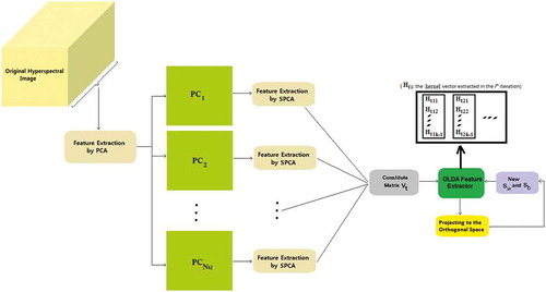
In fact, step 1 provides Nu spectral bands (Nu spectral features) for each pixel. Moreover, step 2 extracts Nu_d spatial features from each . Each is a single band image. So, one can easily apply the SPCA technique to it (see section 3). Now, there are Nu spectral features and spatial features for each pixel. In step 3, the total matrix is constituted. Each column of this matrix represents Nu+ spectral–spatial features of a training sample. Subsequently, OLDA is applied to this matrix for obtaining K−1 kernel vectors .

The block diagram representing the feature extraction methodology is shown in Figure 3. To compare the proposed feature extractor with some recently proposed spectral–spatial feature extraction methods, the extracted features are fed into an SVM classifier.

Support vector machine

SVMs, introduced by Vapnik, have attracted a great deal of interest within the context of statistical learning theory, classification, and function estimation (Vapnik, 1998). This classifier aims at finding the best hyperplane that correctly separates the points of classes and provides maximum margin among them (see Figure 4). SVMs belong to the general group of kernel methods in which the dependency between the kernel and data is described via dot products (Ben-Hur & Weston, 2010). The idea of kernel-based SVM makes it possible to map the training data into a higher dimensional feature space via some mapping and to construct a separating hyperplane there. This hyperplane is a nonlinear decision boundary in the input space. By use of a kernel function , in which and are the input vectors, one can compute the separating hyperplane without mapping the data into a higher dimensional feature space (Howley & Madden, 2004; Zehtabian et al., 2015). Typical choices for kernels are: polynomial kernel, RBF kernel, and sigmoid kernel. In order to classify feature vectors extracted in the previous section, a standard SVM classifier with a polynomial kernel of degree 3 is used:

Figure 4. A linear SVM classifier with maximum margin for the displayed samples (+ and ⊙) consists of the boundary estimate (solid line) and the margin (dotted lines).

(13)

in which , and degree of the kernel (which is three) are the kernel parameters. More details on the SVM classifier can be found in Ben-Hur and Weston (2010), Chang and Lin(2001), Howley and Madden (2004), Vapnik (1998).

Experimental results

The goal of the experimental validation using real data sets is to compare the performance of the proposed method with that reported by the state-of-the-art competitors. The proposed method is applied to three well-known real hyperspectral data sets and the obtained features are used to classify these images. As mentioned before, the classifier used in our experiments is SVM with a polynomial kernel of degree 3.

The SVM classifier is implemented using LIBSVM in which the default kernel parameter values, i.e. γ = 1/(Number of features), and are used (Chang & Lin, 2001). So, very time-consuming tuning techniques such as cross validation or other methods have not been used. A number of labeled samples of each class are randomly selected to train the SVM classifier. In order to study the effect of training sample size on the proposed feature extraction method, we have considered four different proportional schemes: (a) 1%, (b) 5%, (c) 10%, and (d) 12.5% of the labeled samples of each class are used. A point that should be mentioned here is that there are some classes with a small number of labeled samples in the Indian Pines data. To ensure that we have sufficient training samples for the SVM classifier, a minimum of three samples per class is considered in schemes (a) and (b). In other words, for scheme (a) and for scheme (b), where is the number of labeled samples of class i. Although the parameter f is dependent on the spatial structure and texture of the remotely sensed image, this parameter should be large enough to capture the spatial information of the image. The size of f is set to 35 in our experiments (), because the improvement is not significant for a feature extractor with bigger size. In addition, the number of iterations of the algorithm (see step 3) depends on the number of training samples. Our experiments reveal that increasing the number of iterations, when a limited number of training samples are available, does not improve the classification accuracy. The number of iterations for schemes (a),(b), (c), and (d) are set to 7, 10, 15, and 20, respectively, because these values yield good performance in the experiments. For example, in the Indian Pine data set K−1 = 15. So, the number of features is 7 × 15 = 105 for scheme (a), 10 × 15 = 150 for scheme (b), 15 × 15 = 225 for scheme (c), and 20 × 15 = 300 for scheme (d). The number of features for different schemes and data sets is listed in the tables (see Tables 2, 4 and 6).

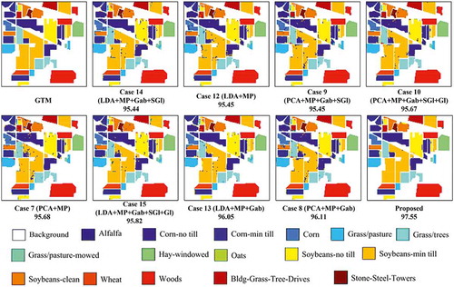
Table 1. Sixteen categories and corresponding number of labeled pixels in the Indian Pines data.

No	Category	Pixels	No.	Category	Pixels
1	Alfalfa	46	9	Oats	20
2	Corn-no till	1428	10	Soybeans-no till	972
3	Corn-min till	830	11	Soybeans-min till	2455
4	Corn	237	12	Soybeans-clean	593
5	Grass/pasture	483	13	Wheat	205
6	Grass/trees	730	14	Woods	1265
7	Grass/pasture-mowed	28	15	Bldg-Grass-Tree-Drives	386
8	Hay-windowed	478	16	Stone-Steel-Towers	93

Table 2. OA, AA, AND KAPPA Statistics () obtained by the SVM classifier on the Indian Pines data. Different combinations of the extracted features are used. the symbol “+” denotes stacking. The number of features is different for different schemes in the proposed method.

			Training set (randomly selected)
			Scheme (a) 1%				Scheme (b) 5%			Scheme (c) 10%			Scheme (d) 12.5%
Case	Input features to SVM	Number of features	OA	AA		OA	AA		OA	AA		OA	AA
1	HS	200	57.81	59.71	51.28	73.66	71.43	69.42	78.89	75.49	75.47	80.34	76.32	77.12
2	HS+MP	251	72.07	73.72	67.75	89.76	87.81	88.09	93.99	92.41	92.99	94.89	92.60	94.03
3	HS+MP+Gab	275	71.59	74.68	67.20	90.64	89.10	89.11	95.26	93.97	94.46	96.01	93.52	95.34
4	HS+MP+Gab+SGl	291	71.81	75.18	67.45	90.48	88.69	88.93	95.20	93.41	94.39	96.10	93.16	95.44
5	HS+MP+Gab+SGl+Gl	307	71.66	75.40	67.22	90.86	89.67	89.36	95.43	93.79	94.66	96.23	93.41	95.59
6	PCA	67	63.96	65.98	58.35	78.19	76.92	74.65	81.82	79.51	78.88	82.87	81.68	80.08
7	PCA+MP	118	77.06	76.95	73.49	92.39	90.52	91.14	95.68	93.49	94.95	95.87	93.25	95.17
8	PCA+MP+Gab	142	73.39	77.10	69.35	92.45	91.07	91.21	96.11	94.38	95.45	96.67	94.90	96.11
9	PCA+MP+Gab+SGl	158	72.33	75.29	68.14	91.56	89.57	90.17	95.45	92.95	94.69	96.10	94.48	95.44
10	PCA+MP+Gab+SGl+Gl	174	70.38	74.43	65.87	91.41	89.65	90.00	95.67	93.47	94.94	96.41	94.57	95.80
11	LDA	15	64.52	67.96	58.67	76.79	76.86	73.06	81.11	76.72	78.06	82.41	79.47	79.53
12	LDA +MP	66	79.19	78.96	75.94	92.97	90.51	91.81	95.45	92.77	94.69	96.11	93.20	95.45
13	LDA +MP+Gab	90	74.58	77.51	70.69	92.54	90.49	91.31	96.05	93.46	95.38	96.97	94.44	96.45
14	LDA +MP+Gab+SGl	106	72.30	75.99	68.10	91.63	89.25	90.24	95.44	92.73	94.67	96.31	93.22	95.68
15	LDA +MP+Gab+SGl+Gl	122	71.84	76.37	67.56	91.77	89.84	90.41	95.82	93.20	95.12	96.48	94.02	95.88
16	Proposed	105–150–225–300	73.33	74.18	68.73	94.47	93.50	93.69	97.55	95.03	97.21	97.84	96.16	97.43

Indian Pines data set

The Indian Pines hyperspectral data set was acquired on 12 June 1992 by the AVIRIS sensor, covering a 2.9 km × 2.9 km portion of Northwest Tippecanoe County, Indiana, USA. Two-thirds of this scene is agriculture, and one-third of it is forest or other natural perennial vegetation. These data include 220 bands with 145 × 145 pixels and a spatial resolution of 20 m. Twenty bands of this data set have been removed because they cover water absorption spectrum band (104–108, 150–163, 220). The corrected data set including 200 bands has been used in our experiments. There are 16 different land-cover classes in the original ground-truth image. Table 1) lists the number of labeled pixels of each class.

Due to the presence of mixed pixels in all available classes and because of the unbalanced number of available labeled pixels per class, this data set constitutes a challenging classification problem (Song et al., 2014).

Several combinations of spectral and spatial features (16 cases) achieving high performance (Mirzapour & Ghassemian, 2015) are fed into the SVM classifier and the classification results are given in Table 2: overall accuracy (OA), average accuracy (AA), and kappa statistics (). Note that the results of tables are obtained by averaging the values obtained in 10 Monte Carlo runs. The abbreviations used in these tables are as follows: HS is the hyperspectral image, MP is the morphological profile, Gab is the Gabor features, Gl is the GLCM (gray-level co-occurrence matrix) features, and SGl is the segmentation-based GLCM features. In addition, Figure 5 shows classification maps for the nine best methods (see Table 2).

Figure 5. Classification results obtained by the SVM classifiers for the AVIRIS Indian Pines scene (using 10% of the available labeled data for the scene).

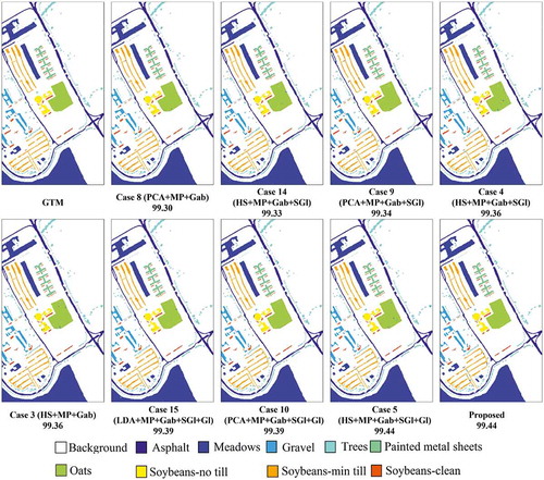
Pavia university data set

In this experiment, the ROSIS Pavia University scene is used to evaluate the proposed approach. This scene was acquired by the ROSIS optical sensor during a flight campaign over the urban area of the University of Pavia, Pavia, Italy. This flight was sponsored by the European Union. It has 103 spectral bands covering the spectral range from 0.43 to 0.86 μm. Each spectral band comprises 610 × 340 pixels with spatial resolution of 1.3 m per pixel. Nine thematic land-cover classes were identified in this scene which are given in Table 3. The OA, AA, and obtained by the SVM classifier are reported in Table 4. Figure 6 shows classification maps for the nine best methods (see Table 4).

Table 3. Nine categories and corresponding number of labeled pixels in Pavia University.

No	Category	Pixels	No.	Category	Pixels
1	Asphalt	6631	6	Oats	5029
2	Meadows	18649	7	Soybeans-no till	1330
3	Gravel	2099	8	Soybeans-min till	3682
4	Trees	3064	9	Soybeans-clean	947
5	Painted metal sheets	1345

Table 4. OA, AA, AND KAPPA Statistics () obtained by the SVM classifier on the Pavia data. Different combinations of the extracted features are used.

			Training set (randomly selected)
			Scheme (a) 1%				Scheme (b) 5%			Scheme (c) 10%			Scheme (d) 12.5%
Case	Input features to SVM	Number of features	OA	AA		OA	AA		OA	AA		OA	AA
1	HS	103	85.40	82.21	80.45	90.48	88.38	87.28	91.67	89.86	88.87	92.00	90.26	89.31
2	HS+MP	154	94.51	92.45	92.66	98.11	97.31	97.47	98.88	98.41	98.50	99.00	98.50	98.66
3	HS+MP+Gab	178	95.23	93.06	93.63	98.77	98.23	98.36	99.36	99.06	99.15	99.42	99.18	99.23
4	HS+MP+Gab+SGl	194	95.26	92.91	93.68	98.87	98.33	98.49	99.36	99.06	99.15	99.45	99.22	99.26
5	HS+MP+Gab+SGl+Gl	210	95.37	93.10	93.83	98.92	98.38	98.56	99.44	99.18	99.25	99.51	99.31	99.34
6	PCA	17	86.23	83.61	81.59	89.28	87.67	85.68	89.46	87.68	85.92	89.85	87.91	86.41
7	PCA+MP	68	93.99	91.61	91.96	97.72	96.64	96.95	98.68	98.05	98.24	98.83	98.29	98.44
8	PCA+MP+Gab	92	94.91	93.01	93.21	98.59	97.92	98.11	99.30	98.92	99.07	99.41	99.12	99.22
9	PCA+MP+Gab+SGl	108	94.70	92.52	92.94	98.70	98.07	98.26	99.34	98.92	99.12	99.46	99.16	99.28
10	PCA+MP+Gab+SGl+Gl	124	94.62	92.77	92.83	98.77	98.16	98.36	99.39	99.01	99.18	99.52	99.24	99.35
11	LDA	8	80.36	78.94	73.77	83.15	81.05	77.29	83.79	81.83	78.22	85.05	81.94	79.65
12	LDA +MP	59	93.63	91.07	91.47	97.85	96.88	97.12	98.58	97.86	98.11	98.79	98.19	98.39
13	LDA +MP+Gab	83	94.57	91.96	92.75	98.52	97.81	98.02	99.26	98.88	99.02	99.43	99.11	99.24
14	LDA +MP+Gab+SGl	99	94.29	91.84	92.38	98.63	97.91	98.18	99.33	98.90	99.11	99.47	99.14	99.30
15	LDA +MP+Gab+SGl+Gl	115	94.25	91.80	92.33	98.74	98.06	98.33	99.39	98.96	99.18	99.52	99.23	99.36
16	Proposed	56–80–120–160	91.2	84.0	88.2	98.73	97.60	98.18	99.44	99.10	99.26	99.62	99.24	99.39

Figure 6. Classification results obtained by the SVM classifiers for the ROSIS Pavia University scene (using 10% of the available labeled data for the scene).

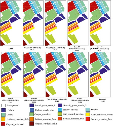
Salinas data set

The Salinas data set includes 224 spectral bands. These data were collected by the AVIRIS sensor over Salinas Valley, California, USA. The image size in pixels is 512 × 217, while the geometric resolution of each pixels is 3.7 m. As with the Indian Pines scene, we discarded the 20 water absorption bands (108–112, 154–167, 224) to obtain a corrected image containing 204 spectral bands. These data include 16 agricultural land covers with very similar spectral signatures (Plaza et al., 2005). The number of labeled pixels of each class is listed in Table 5. The mentioned indices for different schemes are shown in Table 6. The classification maps for the nine best methods are shown in Figure 7 (see Table 6).

Table 5. Sixteen categories and corresponding number of labeled pixels in the Indian Pines data.

No	Category	Pixels	No.	Category	Pixels
1	BBrocoli_green_weeds_1	2009	9	Soil_vinyard_develop	6203
2	BBrocoli_green_weeds_2	3726	10	Corn_senesced_weeds	3278
3	Fallow	1976	11	Lettuce_romaine_4 wk	1068
4	Fallow_rough_plow	1394	12	Lettuce_romaine_5 wk	1927
5	Fallow_smooth	2678	13	Lettuce_romaine_6 wk	916
6	Stubble	3959	14	Lettuce_romaine_7 wk	1070
7	Celery	3579	15	Vinyard_untrained	7268
8	Grapes_untrained	11271	16	Vinyard_vertical_trellis	1807

Table 6. OA, AA, AND KAPPA Statistics () obtained by the SVM classifier on the Salinas data. Different combinations of the extracted features are used.

			Training set (randomly selected)
			Scheme (a) 1%				Scheme (b) 5%			Scheme (c) 10%			Scheme (d) 12.5%
Case	Input features to SVM	Number of features	OA	AA		OA	AA		OA	AA		OA	AA
1	HS	204	88.01	92.88	86.60	90.83	95.76	89.75	91.99	96.49	91.05	92.18	96.54	91.25
2	HS+MP	255	95.15	96.51	94.58	97.88	98.68	97.63	98.36	99.05	98.17	98.57	99.17	98.40
3	HS+MP+Gab	279	95.08	96.58	94.50	98.22	98.88	98.01	98.83	99.32	98.70	99.03	99.41	98.91
4	HS+MP+Gab+SGl	295	95.76	96.90	95.26	98.42	98.86	98.24	99.10	99.38	99.00	99.21	99.45	99.12
5	HS+MP+Gab+SGl+Gl	311	95.82	96.95	95.33	98.57	98.95	98.40	99.24	99.44	99.15	99.38	99.52	99.31
6	PCA	6	87.72	92.27	86.26	90.13	94.63	88.95	90.09	95.05	88.92	90.62	95.34	89.50
7	PCA+MP	57	93.78	94.99	93.04	97.52	98.02	97.23	98.32	98.77	98.12	98.60	99.00	98.43
8	PCA+MP+Gab	81	94.01	95.37	93.30	98.03	98.53	97.80	98.82	99.19	98.67	99.03	99.39	98.91
9	PCA+MP+Gab+SGl	97	95.12	96.20	94.55	98.23	98.67	98.02	99.01	99.25	98.89	99.19	99.42	99.09
10	PCA+MP+Gab+SGl+Gl	113	94.86	96.04	94.26	98.36	98.73	98.17	99.01	99.26	98.89	99.23	99.44	99.14
11	LDA	15	89.18	94.05	87.91	92.21	96.14	91.29	93.03	96.68	92.19	93.25	96.83	92.45
12	LDA +MP	66	93.88	95.32	93.16	97.65	98.18	97.37	98.42	98.77	98.23	98.58	98.89	98.41
13	LDA +MP+Gab	90	94.18	95.66	93.49	98.00	98.53	97.77	98.86	99.23	98.73	99.04	99.35	98.93
14	LDA +MP+Gab+SGl	106	95.30	96.47	94.75	98.26	98.70	98.06	99.01	99.23	98.90	99.25	99.44	99.16
15	LDA +MP+Gab+SGl+Gl	122	95.11	96.34	94.53	98.31	98.72	98.11	99.06	99.29	98.95	99.27	99.45	99.19
16	Proposed	105–150–225–300	96.02	97.36	95.58	99.39	99.67	99.26	99.85	99.88	99.83	99.92	99.91	99.83

Figure 7. Classification results obtained by the SVM classifiers for the Salinas data set (using 10% of the available labeled data for the scene).

Discussing the results

In this subsection, we will discuss the classification results for various combinations of spatial and spectral features used in the experiments. Then, we compare the performance of the proposed method with that of competing methods. From these tables, one can see that the best accuracies for the same data set with different training schemes correspond to different features. In other words, there may not be found a unique feature extraction method which gives the best results for different number of training samples even for the same data set. Besides, for different data sets, the best cases corresponding to the same number of training samples are different. So, it seems that finding a unique feature extraction method which gives the best results for different training schemes and for different data sets, is difficult. In fact, it is not far from the truth to say that there does not exist such a feature extraction method (Kuo, Li, & Yang, 2009). However, because the coefficients of the proposed method depend on the training samples of the data, it should be more consistent with the characteristics of the images. In other words, it is less sensitive to the different data sets compared with unsupervised methods such as PCA, Gabor, and morphological filters.

As can be seen from the tables, the proposed features are the best ones in the schemes (b), (c), and (d) for the Indian Pines data, and in schemes (a), (b), (c), and (d) for the Salinas data. However, for the Pavia University data set, the proposed features are the best ones only in schemes (c) and (d) (except for AA criterion). These results reveal that the proposed features are almost certainly the best ones when there are enough training samples. Because the coefficients of the proposed feature extractor are estimated from the training samples, the more the training samples are available, the more accurate coefficients are estimated. In parametric methods, e.g. the proposed feature extractor, the availability of training samples is very important such that when the number of training samples is very small, simple unsupervised feature extractors, e.g. PCA and Gabor filters, have better performance. This is because of the overfitting that typically occurs in unsupervised methods. So, in parametric feature extraction methods, e.g. the proposed method, the number of training samples plays a vital role. However, because the OLDA is used in our methodology, which is less sensitive to the overfitting and limited number of training samples, the proposed method has the best performance in schemes (a) and (b) for the Salinas data set and in scheme (b) for the Indian Pines data set.

At the end of this section, we provide a comparative assessment. The proposed algorithm is compared with some recently proposed spectral–spatial classification methods. To do a reliable comparison, the classification results for SVM-CK (Camps-Valls, Gomez-Chova, Muñoz-Marí, Vila-Francés, & Calpe-Maravilla, 2006) are obtained by implementing the algorithm using the publicly available codes. But, the results for other methods are reported from the corresponding papers. Thus, some results are absent. The results of this comparison are given in Table 7. As can be seen from this table, the proposed method outperforms other methods in schemes (c) and (d), i.e. when the number of training samples is large. Moreover, the proposed method outperforms other methods in scheme (b) for the Salinas data, i.e. when the number of training samples is moderate. In addition, Table 8 reports the computational time of the proposed method using a standard notebook (Intel Core i5, 2.66 GHz and 4 GB of RAM) for different data sets (each experiment is repeated 10 times and the average is reported). As can be seen from this table, the computational complexity of the proposed method is moderate.

Table 7. Overall accuracies of the proposed method compared to some recently proposed classification methods.

Data set	Number of training samples%	Diverse AdaBoost SVM†^a	FODPSO + MSS (R = 5) + SVM^b	EMAP (KPCA)+RF classifier^c	SUnSALEMAP	SVM CK^d	Proposed
Indian Pines	1	–	–	–	–	73.7	73.3
	5	–	–	88.7	95.0	91.4	94.5
	10	92.6	–	92.7	96.8	94.9	97.6
	12.5	–	–	–	–	95.8	97.8
Pavia University	1	–	–	–	86.0	95.3	91.2
	5	–	–	98.8	–	98.3	98.7
	10	95.7	–	–	97.5	98.5	99.4
	12.5	–	98.9	–	–	98.6	99.6
Salinas	1	–	–	–	–	95.6	96.0
	5	–	–	–	–	98.7	99.4
	10	94.9	–	–	–	98.9	99.9
	12.5	–	99.1	–	–	99.1	99.9

^aReported from Ramzi, Samadzadegan, and Reinartz (2013). ^b Reported from Ghamisi, Couceiro, Fauvel, and Benediktsson (2014). ^c Reported from Bernabé, Marpu, and Plaza (2014). ¶ Reported from Song et al. (2014). ^d Reported from Camps-Valls et al. (2006).

Table 8. Mean of the computation time for different data sets (10% of the labeled samples of each class are used as training samples).

Data sets	Number of extracted features	Time (S)
Indian Pines	225	24.12
Pavia	120	50.83
Salinas	225	62.74

Conclusion

This paper first proposes a new filter bank able to extract the spatial information of hyperspectral images. Then, a new supervised feature extraction technique is proposed in Section 4, which takes into account both the spatial and spectral information simultaneously. To obtain the coefficients of the feature extractor, the Fisher score is maximized. To this end, and to overcome the singularity problem, the OLDA method is used which is less susceptible to overfitting and is more robust against noise. To reduce the dimensionality of the feature matrix, the PCA transform is used as a preprocessing step. The steps of the proposed method are (1) applying PCA in the spectral domain, (2) applying PCA in the spatial domain, (3) extracting the best spectral–spatial features in terms of class separability using OLDA. Due to the fact that the number of extracted features is not sufficient for classification, the orthogonalization process is iterated (by the Gram–Schmidt algorithm) until the sufficient number of features is provided. To compare the performance of the proposed method with that of other methods, the extracted features were classified using an SVM classifier with a polynomial kernel of degree 3. Three real hyperspectral data sets, namely Indian Pines, Pavia University, and Salinas were used in our experiments. In addition, to investigate the influence of the size of training set on the feature extraction methods, we adopted four different schemes for the number of training samples. The experimental results have demonstrated that the proposed feature extraction method can provide excellent features for the classification purpose when the number of training samples is large enough. Finally, the proposed method was compared with some recently proposed spectral–spatial classification methods. The comparative results confirm the good capabilities of the proposed method.

Disclosure statement

No potential conflict of interest was reported by the authors

References

- Aguilar, M.A., Fernández, A., Aguilar, F.J., Bianconi, F., & Lorca, A.G. (2016). Classification of urban areas from GeoEye-1 imagery through texture features based on histograms of equivalent patterns. European Journal of Remote Sensing, 49, 93–120. doi:10.5721/EuJRS20164906
- Bandos, T., Bruzzone, L., & Camps-Valls, G. (2009, Mar). Classification of hyperspectral images with regularized linear discriminant analysis. IEEE Transactions on Geoscience and Remote Sensing, 47(3), 862–873. http://ieeexplore.ieee.org/xpls/abs_all.jsp?arnumber=4786582
- Bayliss, J., Gualtieri, J.A., & Cromp, R. (1997). Analysing hyperspectral data with independent component analysis. Proceedings SPIE, 3240, 133–143. http://proceedings.spiedigitallibrary.org/proceeding.aspx?articleid=933255
- Benediktsson, J.A., Palmason, J.A., & Sveinsson, J.R. (2005, Mar). Classification of hyperspectral data from urban areas based on extended morphological profiles. IEEE Transactions on Geoscience and Remote Sensing, 43(3), 480–491. http://ieeexplore.ieee.org/xpls/abs_all.jsp?arnumber=1396321
- Ben-Hur, A., & Weston, J. (2010). A user’s guide to support vector machines. Methods in Molecular Biology (Clifton, N.J.), 609, 223–239. http://link.springer.com/protocol/10.1007/978-1-60327-241-4_13
- Bernabé, S., Marpu, P.R., & Plaza, A. (2014, Jan). Spectral–spatial classification of multispectral images using kernel feature space representation. IEEE Transactions on Geoscience and Remote Sensing, 11(1), 288–292. http://ieeexplore.ieee.org/xpls/abs_all.jsp?arnumber=6524967
- Camps-Valls, G., & Bruzzone, L. (2005, Jun). Kernel-based methods for hyperspectral image classification. IEEE Transactions on Geoscience and Remote Sensing, 43(6), 1351–1362. http://ieeexplore.ieee.org/xpls/abs_all.jsp?arnumber=1433032
- Camps-Valls, G., Gomez-Chova, L., Muñoz-Marí, J., Vila-Francés, J., & Calpe-Maravilla, J. (2006, Jan). Composite kernels for hyperspectral image classification. IEEE Transactions on Geoscience and Remote Sensing, 3(1), 93–97. http://ieeexplore.ieee.org/xpls/abs_all.jsp?arnumber=1576697
- Chang, -C.-C., & Lin, C.-J. (2001). LIBSVM: A Library for Support Vector Machines [Online]. Available: http://www.csie.ntu.edu.tw/~cjlin/libsvm
- Cheng, G., Han, J., Guo, L., Liu, Z., Bu, S., & Ren, J. (2015, Aug). Effective and efficient midlevel visual elements-oriented land-use classification using VHR remote sensing images. IEEE Transactions on Geoscience and Remote Sensing, 53(8), 4238–4249. http://ieeexplore.ieee.org/document/7046387
- Cheng, G., Han, J., Zhou, P., & Guo, L. (2014). Multi-class geospatial object detection and geographic image classification based on collection of part detectors. ISPRS Journal of Photogrammetry and Remote Sensing, 98, 119–132. doi:10.1016/j.isprsjprs.2014.10.002
- Cheng, G., Zhou, P., & Han, J. (2016). RIFD-CNN: Rotation-invariant and fisher discriminative convolutional neural networks for object detection. In Proceedings of the IEEE Conference on Computer Vision and Pattern Recognition, 2884–2893. http://www.cv-foundation.org/openaccess/content_cvpr_2016/html/Cheng_RIFD-CNN_Rotation-Invariant_and_CVPR_2016_paper.html
- Ghamisi, P., Couceiro, M., Fauvel, M., & Benediktsson, J.A. (2014, Jan). Integration of segmentation techniques for classification of hyperspectral images. IEEE Transactions on Geoscience and Remote Sensing, 11(1), 342–346. https://www.researchgate.net/profile/Micael_Couceiro/publication/260541108_Integration_of_Segmentation_Techniques_for_Classification_of_Hyperspectral_Images/links/02e7e533775b5effef000000.pdf
- Green, R.O., et al. (1998). Imaging spectroscopy and the airborne visible/infrared imaging spectrometer (AVIRIS). Remote Sensing of Environment, 65, 227–248. doi:10.1016/S0034-4257(98)00064-9
- Howley, T., & Madden, M.G. (2004). “The genetic evolution of kernels for support vector machine classifiers,” In Proceedings of 15th Irish Conference on Artificial Intelligence and Cognitive Science. http://citeseerx.ist.psu.edu/viewdoc/download?doi=10.1.1.81.4119&rep=rep1&type=pdf
- Kuo, B.C., Ho, H.H., Li, C.H., Hung, C.C., & Taur, J.S. (2014, Jan). A kernel-based feature selection method for SVM with RBF kernel for hyperspectral image classification. IEEE Journal of Selected Topics in Applied Earth Observations and Remote Sensing, 7(1), 317–326. http://ieeexplore.ieee.org/document/6521421
- Kuo, B.C., Li, C.H., & Yang, J.-M. (2009, Apr). Kernel nonparametric weighted feature extraction for hyperspectral image classification. IEEE Transactions on Geoscience and Remote Sensing, 47(4), 1139–1155. http://ieeexplore.ieee.org/xpls/abs_all.jsp?arnumber=4801616
- Li, J., Huang, X., Gamba, P., Bioucas, J., Zhang, L., Benediksson, J., & Plaza, A. (2015, Mar). Multiple feature learning for hyperspectral image classification. IEEE Transactions Geoscience and Remote Sensing, 53,(3), 1592–1606. http://ieeexplore.ieee.org/xpls/abs_all.jsp?arnumber=6882821
- Ma, L., Crawford, M.M., & Tian, J. (2010, Nov). Local manifold learning-based k-nearest-neighbor for hyperspectral image classification. IEEE Transactions on Geoscience and Remote Sensing, 48(11), 4099–4109. http://ieeexplore.ieee.org/xpls/abs_all.jsp?arnumber=5555996
- Mirzapour, F., & Ghassemian, H. (2015, Mar). Improving hyperspectral image classification by combining spectral, texture, and shape features. International Journal of Remote Sensing, 36(4), 1070–1096. http://www.tandfonline.com/doi/abs/10.1080/01431161.2015.1007251
- Nagabhatla, N., & Kühle, P. (2016). Tropical agrarian landscape classification using high-resolution GeoEYE data and segmentationbased approach. European Journal of Remote Sensing, 49, 623–642. doi:10.5721/EuJRS20164933
- Okada, T., & Tomita, S. (1985). An optimal orthonormal system for discriminant analysis. Pattern Recognition, 18, 139–144. doi:10.1016/0031-3203(85)90037-8
- Plaza, A. et al. (2009, Sep). Recent advances in techniques for hyperspectral image processing. Remote Sensing of Environment, 113(Suppl. 1), 110–122. http://www.sciencedirect.com/science/article/pii/S0034425709000807
- Plaza, A., Martinez, P., Plaza, J., & Perez, R. (2005, Mar). Dimensionality reduction and classification of hyperspectral image data using sequences of extended morphological transformations. IEEE Transactions on Geoscience and Remote Sensing, 43(3), 466–479. http://ieeexplore.ieee.org/xpls/abs_all.jsp?arnumber=1396320
- Ramzi, P., Samadzadegan, F., & Reinartz, P. (2013, Dec). Classification of hyperspectral data using an AdaBoost SVM technique applied on band clusters. IEEE Journal of Selected Topics in Applied Earth Observations and Remote Sensing, 7(6), 2066–2079. http://ieeexplore.ieee.org/xpls/abs_all.jsp?arnumber=6691910
- Song, B., Li, J., Dalla-Mura, M., Li, P., Plaza, A., Bioucas-Dias, J.M. … Chanussot, J. (2014, Aug). Remotely sensed image classification using sparse representations of morphological attribute profiles. IEEE Transactions on Geoscience and Remote Sensing, 52(8), 5122–5136. http://ieeexplore.ieee.org/xpls/abs_all.jsp?arnumber=6674087
- Su, T.C. (2016). A filter-based post-processing technique for improving homogeneity of pixel-wise classification data. European Journal of Remote Sensing, 49, 531–552. doi:10.5721/EuJRS20164928
- Vapnik, V.N. (1998, Sep). Statistical Learning Theory. New York, NY: John Wiley &Sons. http://www.dsi.unive.it/~pelillo/Didattica/Artificial%20Intelligence/Old%20Stuff/Slides/SLT.pdf
- Yang, J., & Yang., J.U. (2003, Feb). Why can LDA be performed in PCA transformed space? Pattern Recognition, 36(2), 563–566. http://www.sciencedirect.com/science/article/pii/S0031320302000481
- Ye, J. (2005, Dec). Characterization of a family of algorithms for generalized discriminant analysis on undersampled problems. Journal Mach Learning Researcher, 6, 483–502. http://www.jmlr.org/papers/v6/ye05a.html
- Ye, J., Janarda, R., Li, Q., & Park, H. (2006, Oct). Feature reduction via generalized uncorrelated linear discriminant analysis. IEEE Transactions on Knowledge and Data Engineering, 18(10), 1312–1322. http://ieeexplore.ieee.org/xpls/abs_all.jsp?arnumber=1683768
- Ye, J., & Xiong, T. (2006a). Null space versus orthogonal linear discriminant analysis. Proceedings ACM International Conference Machine Learning, 1073–1080. http://dl.acm.org/citation.cfm?id=1143979
- Ye, J., & Xiong, T. (2006b, Jul). Computational and theoretical analysis of null space and orthogonal linear discriminant analysis. Journal Mach Learning Researcher, 7, 1183–1204. http://www.jmlr.org/papers/v7/ye06a.html
- Zehtabian, A., & Ghassemian, H., 2016. Automatic object-based hyperspectral image classification using complex diffusions and a new distance metric. ieee transactions on geoscience and remote sensing, 54(7), 4106–4114.
- Zehtabian, A., Nazari, A., Ghassemian, H., & Gribaudo, M., 2015. Adaptive restoration of multispectral datasets used for svm classification. European Journal Of Remote Sensing, 48, 183–200.