A novel method for urban land cover mapping based on new vegetation indices and texture-spectral information from fused visible and hyperspectral thermal infrared airborne data

ABSTRACT

Update information on urban regions has been substantial for management communities. In this research, a novel method was developed for Urban Land Cover Mapping (ULCM). Textural-spectral features obtained from Hyperspectral Thermal Infrared (HTIR) data were fused with spatial-spectral features of the visible image for ULCM. The proposed method consists of three hierarchical steps. First, trees and vegetation classes were classified based on spatial-spectral features extracted from the visible image. Also, two new vegetation indices were introduced. By studying spectral signatures of trees and vegetation classes on the HTIR data, it was shown that trees and vegetation classes could be discriminated by visible data. Second, textural-spectral features of the HTIR data were fused with visible image features to extract bare soil, (gray; concrete; red) roof buildings and roads classes. Using HTIR textural features increased the overall accuracy and Kappa coefficient values about 6% and 8% correspondingly. Third, the results of the first and second steps were overlaid and post processing has been done. The obtained results for overall accuracy and Kappa coefficient values were 94.96% and 0.928 respectively. The comparison of the achieved results with the results of the contest announced by IEEE has shown the efficiency of the proposed method.

KEYWORDS:

• Hyperspectral thermal infrared
• urban land cover mapping
• vegetation index
• visible image

Introduction

Urban objects and urban land cover maps are crucial geospatial data required by many organizations such as urban planners, municipalities, service centers, so on. Geomatics sciences have been one of the major providers of urban geospatial information (Mohammadzadeh, Zoej, & Tavakoli, 2008); (Cockx, Van De Voorde, & Canters, 2014). Remote sensing (RS) sensors provide efficient data on the earth surface (Sarp, Erener, Duzgun, & Sahin, 2014; Aguilar, Fernández, Aguilar, Bianconi, & Lorca, 2016; Uzar, 2014).

Up to now, a variety of RS sensors have provided different types of data which have been used for urban objects detection and classification (Cockx et al., 2014; Benediktsson, Pesaresi, & Amason, 2003; Rottensteiner et al., 2014; Guo, Chehata, Mallet, & Boukir, 2011). Thermal infrared (TIR) images have been used in a wide range of applications (Kuenzer & Dech, 2013; Prakash, 2000). Recently, a revolution has happened in the spatial and spectral resolution of the TIR data and made it suitable for the urban land cover mapping (ULCM) investigators. In the other research, authors applied a fused method on the fusion of LiDAR, optical and TIR data for urban structure and environment monitoring (Brook, Vandewal, & Ben-Dor, 2012). Accordingly, in their proposed strategy, more attention was given for using LiDAR and optical data, while multiband TIR data contain useful information for urban object detection applications. Few researchers used high spatial resolution hyperspectral thermal infrared (HSR-HTIR) data and very high spatial resolution (VHSR) visible aerial image for ULCM operations (Liao et al.). Consequently, in their works, many spatial feature spaces were extracted from VHSR visible image. After that, principal component analysis band reduction method was applied on HSR-HTIR data and some bands were selected. Then spatial–spectral bands of the visible image and spectral bands of TIR data were fed to Support Vector Machine (SVM) classifier for ULCM (Liao et al.). In our previous work, we developed a spectral-based strategy on the fused HSR-HTIR and visible data for urban object detection (Eslami & Mohammadzadeh, 2016). In our work, first atmospheric correction and band reduction approaches were applied on the HSR-HTIR data. Then, estimated TIR spectral features and three spectral bands of the visible image were fused and fed to a SVM classifier, and seven desired urban classes of bare soil (red, gray, concrete) roof buildings, roads, trees and vegetation were produced.

In the aforementioned works, more weight was given to the visible image in ULCM applications and extracted spatial features from the visible image have been broadly used, while the spatial features derived from the TIR data were not studied for improvement of the urban land cover classification accuracy. Likewise, there is lack of comprehensive studies about the performance of the TIR data for urban object detection applications.

In this paper, a comprehensive and novel textural–spectral-based method was developed for fusion of VHSR visible and HSR-HTIR airborne data for classification and mapping of urban objects. To the best of the authors’ knowledge, this is the first time that the potential of the HSR-HTIR data was studied and analyzed for discrimination of trees and vegetation classes. In this paper again for the first time, textural features were extracted from HSR-TIR data and tested for accuracy improvement of the ULCM applications, while in the aforementioned works they used only spectral features of this data. Furthermore, two new vegetation indices (VIs) which were extracted from only bands in the visible part of the spectrum were introduced and tested.

The novel hierarchical method which was proposed in this article consists of three main steps and was designed for mapping of seven urban classes: bare soil (red, gray, concrete) roof buildings, roads, trees and vegetation. Trees and vegetation were separated by textural-, spectral- and novel-introduced VIs, which were extracted from visible image. Afterward, a band reduction method was applied on the HSR-HTIR and nine bands were selected. Then, textural features were extracted from TIR data. After that, textural and spectral features of visible and TIR data were fed to an SVM classifier and five urban classes (i.e. bare soil (red, gray, concrete), roof buildings and roads) were classified. Finally, the outcome of the previous steps was combined and fed to post-processing method and produced final urban land cover map. The performance of the proposed strategy was contrasted with the best results of the 2014 data fusion contest announced by IEEE Geoscience and Remote Sensing Society (GRSS) (Liao, et al.).

The rest of the article is structured into four sections as follows. In the second section, the flowchart of the proposed method was discussed and illustrated. Third section presented a description of the gray-level co-occurrence matrix (GLCM), sequential parametric projection pursuit (SPPP) band reduction, SVM and maximum likelihood classifier (MLC) methods. Fourth section gave information on the experimental results, followed by a discussion of the proposed method. Finally, the concluding remarks were given in the fifth section.

Algorithm description

The flowchart of the proposed strategy is shown in Figure 1. The proposed hierarchical method contains three main steps. In the first step: two newly introduced VIs which named subdividing vegetation index (SVI) and minus/subdividing vegetation index (MSVI) were calculated from visible image. Then, 24 textural features based on GLCM were extracted. After that, maximum noise fraction (MNF) band reduction method was applied to the outcome of GLCM bands and five first bands were selected. Finally, three spectral bands of visible image, five bands of the MNF output and two bands of newly proposed VIs were fed to an MLC method. In the first step, trees and vegetation classes’ maps were separated.

Figure 1. Proposed hierarchical strategy.

In the second step, SPPP band reduction method was applied to the HSR-HTIR data and nine spectral bands were estimated. Then textural features by GLCM were calculated on the nine bands of the TIR data. Furthermore, an MNF method was applied to the results of the GLCM statistical feature extraction methods’ bands and five first bands were selected. Finally, an SVM classification approach was applied to the combined nine spectral bands of TIR data, five textural bands of the MNF output of the GLCM statistics on the TIR data, three spectral bands of visible image and five textural bands of the MNF method on the visible image. In this step, five urban classes (bare soil (red, concrete, gray), roof buildings and roads) were detected. In the third step, the resultant maps of the first and second steps were combined and produced ULCM map in the seven interest classes. Then object-rule-based post-processing (ORBPP) method was applied to the classified map and final ULCM map was produced.

Methods and materials

In this section, statistical feature extraction methods based on GLCM are described. Then, MNF and SPPP approaches, two well-known bands reduction methods, are defined. Also, a brief description of the SVM classification method is provided. Moreover, SVI and MSVI VIs are introduced.

Gray-level co-occurrence matrix

The texture consists of the significant information about a surface relationship to the adjacent environment and their structural arrangement (Haralick, Shanmugam, & Dinstein, 1973). The GLCM features are categorized as a second-order statistical texture feature extraction method (Albregtsen, 2008). In GLCM number of columns and rows are estimated based on the number of gray levels in the image (Albregtsen, 2008). The elements of GLCM matrix shows the statistical estimated values which happen between the gray-level value i and j at a special direction θ and distance d (Haralick et al., 1973). Various textural features can be estimated based on GLCM matrix. In this paper, eight texture features are used: entropy, variance, contrast, correlation, angular second moment (ASM), mean, homogeneity and dissimilarity.

Entropy shows the rate of the homogeneous in an image scene. An image with higher entropy value has homogeneous scene (Albregtsen, 2008). The entropy defines as follows:

(1)

Other texture features can be found in Albregtsen (2008 and Soh and Tsatsoulis (1999).

Maximum noise fraction

Band reduction methods can be categorized in two main groups, that is, supervised and unsupervised (Patra, Modi, & Bruzzone, 2015). MNF is a linear unsupervised band reduction method which transforms hyperspectral original data into a second feature space with a higher value of the signal to noise ratio (Green, Berman, Switzer, & Craig, 1988).

For “M” bands in original space, every pixel contains one vector of the gray values defines as Z_n = (z₁,…, z_m). Further, let N_n and S_n be uncorrelated noise and signal components, respectively. According to additive model Z_n defines as follows (Amato, Cavalli, Palombo, Pignatti, & Santini, 2009):

(2)

Let we assume ∑_S and ∑_N as covariance matrices of signal and noise, respectively. The process seeks an A such that Equation (3) be correct:

(3)

Finally, the MNF transform matrix is defined by

(4)

By estimation of H, original space transforms the second space as follows (Amato et al., 2009):

(5)

Sequential parametric projection pursuit

In classification methods, an extreme number of bands provide more information for separation of the different classes, but the limited number of training data, based on Hughes phenomenon, will reduce the classification accuracy (Hughes, 1968). Therefore, to increase the classification accuracy in attention to the Hughes phenomenon on the HSR-HTIR Eslami and Mohammadzadeh (2016) proposed SPPP bands reduction method. SPPP band reduction method transforms original hyperspectral space X to the second multiband space Y by estimation of the optimized matrix A, as shown in Equation (6) (Lin & Bruce, 2003):

(6)

Estimation of the optimized A is based on the optimization of a Projection Index (PI). Among variety of the PI approaches reported by Lin and Bruce (2003) and Geman and Geman (1984), we used Bhattacharyya distance (BD). BD uses standard deviation and mean values of different classes to be estimated as follows:

(7)

where, the mean values and covariance matrices of the classes i and j are M_i, M_j, and respectively and B_ij is the BD value. The process of the SPPP bands reduction method is described as follows:

Distribute original space spectral bands to S groups. Then, generate matrix A as 8, with S columns and R rows. R is the number of bands in original space. In the matrix A, position of the elements fills as , q = 1: S and, l = 1:N.

(8)

1. Matrix A optimizes, starting through the first group of nearby bands, that is, changing values that maximizes the BD value with the nonzero elements in the first column of the matrix A, while preserving the remain columns of the matrix A unchanged. The replacing of the nonzero elements of A will be done from the matching bank of the group of the nearby bands, which is described in Eslami et al. (2015).

2. For every remaining group of the nearby bands in the matrix A, repeat step (2).

3. Until the growth in BD value is below an identified threshold or is not substantial, repeat steps (2) and (3). Again, the replacing of the nonzero elements of A will be done from the matching bank of the group of the nearby bands.

4. Apply top-down approach to raise the number of the groups one by one. Then repeat steps (2), (3) and (4).

5. Until the growth in BD value is below an identified threshold or not substantial, repeat step (5).

Support vector machine

SVM is a statistical supervised nonparametric classification method. If , and are the feature vectors of training data. X, in the feature space, n is the dimension of feature space. SVM classification method leads to a hyperplane as Equation (9) to discriminate feature vectors into two different classes (Mountrakis, Im, & Ogole, 2011; Theodoridis, Pikrakis, Koutroumbas, & Cavouras, 2010), where, w_p and w₀ are the hyperplane equation coefficients. Furthermore, SVM needs lesser training data and has higher accuracy in comparison to the other classifiers (Theodoridis et al., 2010). SVM uses just support vectors for estimation of the separating hyperplane while maximizing the Margin (Bovolo, Camps-Valls, & Bruzzone, 2007). Separation hyperplane can be defined as linear or nonlinear in attention to the performance of the hyperplane in the separation of the multifeature space. If it not separated by linear one, method uses soft margin and kernels for increasing accuracy of the classification results (Burges, 1998).

(9)

In image-processing applications, the pixel belongs to one of the two interest classes by identification of the SVM classifier. As multiclass classification needs another strategy, pairwise classification method was assumed for this study. Under pairwise classification method, for every pair of classes a binary SVM classification was applied. If the number of classes is V, the final number of single SVM classification equals to V(V–1)/2 (Richards & Richards, 1999). Finally, the pixel is labeled to the class with the highest recommendation value of classification.

SVI and MSVI

VIs have been shown to have an undeniable role for increasing accuracy of classification methods (Lopes et al., 2015). The most popular VI methods have been widely used, which were extracted from the combination of the visible and near infrared (NIR) spectral bands (Bannari, Morin, Bonn, & Huete, 1995). By lack of NIR bands, VIs based on visible bands have been employed (Lopes et al., 2015; Gitelson, 2004) while there is not given full consideration to the combination of blue and green bands. Therefore, in this study two new VI methods which named SVI and MSVI were proposed. SVI was estimated as shown in Equation (10) and MSVI was calculated as shown in Equation (11) while B and G are blue and green bands of the visible image, respectively. In the visible region of electromagnetic waves, vegetation’s highest reflectance happens in the green band, which gives increase to the green color of vegetation. The reflectance is low in the blue band of the spectrum because of absorption by chlorophyll for photosynthesis (Knipling, 1970). We tried to use high and low reflectance bands combination as follows for vegetation discrimination in the act of new VI. The newly proposed VI methods use a threshold value to discriminate the vegetation classes; also, it can be used as a further feature space in the classification applications..

(10)

(11)

Experimental results and discussion

In this section, the effectiveness of the proposed method is evaluated. Later, data sets, implementation criteria and experimental results are discussed.

Study area and data set

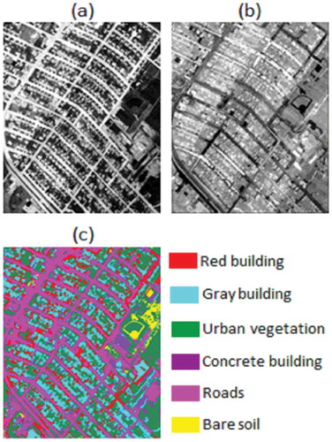
The data set of this study was provided for the Data Fusion Contest 2014 by the Image Analysis and Data Fusion (IADF) Technical Committee of the IEEE GRSS. The data were obtained by TELOPS (Canada) corporation on the urban area near Thetford Mines in Québec. The data had been acquired on 21 May 2013 with averagely 807 m height of airborne sensors above ground. Likewise, the average temperature of the study area was 13°C. Visible image was the first set of data with 0.2 m spatial resolution and is shown in Figure 2(a). The second one which covers 7.8–11.5 µm wavelengths was HSR-HTIR data with 84 spectral bands with about 1 m spatial resolution and is shown in Figure 2(b). Bands 81–84 of HSR-HTIR data are very noisy and were not used in this research study. Until now this kind of data is a unique data set, so we tested our proposed strategy only on the one study area.

Figure 2. Visible image (a), thermal data (b), train data set (c) and test data set (d)..

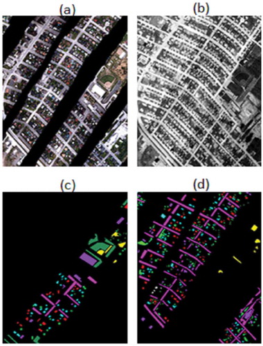
The train and test data of the mentioned data fusion contest were used for training and evaluation of the proposed method as shown in Figure 2(c, d). Also, we divided train data into group 1 (with 20% of the training data) and group 2 (with 80% of the training data). Groups 1 and 2 were used for training, evaluation and optimization of the proposed method. Finally, the test data were applied to the final assessment of the proposed method.

First step, trees and vegetation discrimination

As mentioned previously, in this step, five urban classes: bare soil (gray, red, concrete), roof buildings and roads were blended into “urban objects” class. In fact, the final of this step was the classification of three main classes: trees, vegetation and “urban objects”. First, SVI and MSVI were estimated based on Equations (10) and (11). In Figure 3, the SVI and MSVI are shown.

Figure 3. MSVI band (a), first MNF band (b), SVI band (c) and final classification map (d).

Second, eight textural features were extracted, which consist of entropy, variance, contrast, correlation, ASM, mean, homogeneity and dissimilarity. For each band of the visible image, every textural feature was estimated in four directions (0°, 45°, 90° and 135°). Furthermore, other parameters of the texture window were fixed as 1 pixel and 7 pixels to the distance and window size, respectively. Then, according to Haralick et al. (1973), the average of the mentioned four direction bands was estimated to every textural feature. Last, 24 texture features were produced from three bands of the visible image. Then MNF band reduction method was applied to the outcome of those 24 bands, and five first bands are selected (see Figure 3(b)). Third, three spectral bands of the visible image, five textural features of MNF outcome and two newly proposed VIs were fed to the MLC classifier and final map of the first step produced (see Figure 3(d)).

In Table 1 the error matrix of the final produced map in first step was shown. Furthermore, for evaluation of the produced results in the first step, three bands of the visible image were individually fed to MLC, and the error matrix is shown in Table 1. By comparing the results of the first step against the results of using only visible bands, there were about 4%, 14% and 15% increase in the overall accuracy, Kappa coefficient and average accuracy, respectively, for the used strategy in the first step. Also, the correlation between trees and vegetation classes was descended by using the proposed strategy in the first step. Furthermore, the trees and vegetation classes’ accuracies were increased about 34% and 11%, respectively while the “urban objects” class’ accuracy was not changed significantly.

Table 1. Error matrix of the final map in the first step comprising to use of just spectral bands of the visible bands (percentage).

		Actual class
	Method	Class name	Trees	Vegetation	Urban objects	Accuracy
Predicted class	Final map	Trees	93.38	11.08	0.31	Overall: 98.51
		Vegetation	6.45	88.51	0.09	Kappa: 0.9303
		Urban objects	0.16	0.41	99.60	Average: 93.83
	Visible only	Trees	82.17	44.75	0.56	Overall: 94
		Vegetation	17.69	54.67	0.27	Kappa: 0.7921
		Urban objects	0.13	0.58	99.17	Average: 78.67

For further evaluation of the two newly proposed VIs, two individual classifications were applied to the combination of the three visible bands with SVI and MSVI separately. The obtained results as the error matrix were shown in Table 2. The obtained results revealed the significant performance of the proposed indices in comparison to using only visible bands case. Likewise, for further association of the SVI and MSVI performances, three well-known VI methods based on visible image bands – Vegetation Index Green (VIgreen), VARIgreen (Gitelson, Kaufman, Stark, & Rundquist, 2002) and Excess Green (EG) (Lopes et al., 2015) – were individually combined with visible image bands and classified with the same conditions to the mentioned SVI and MSVI. Obtained results were compared in Table 2 and were shown the efficiency and productivity of the two newly proposed VIs. According to Table 2, SVI had the best results in terms of the overall accuracy and Kappa coefficient about 95.77% and 0.8324, respectively. The MSVI has shown better average accuracy comparing to the results obtained by other VI methods. Further, SVI and MSVI improved the accuracy of the vegetation class, while other VI methods have shown more correlation between trees and vegetation classes.

Table 2. Error matrix for SVI, MSVI, VIgreen, VARIgreen and EG vegetation index methods.

		Actual class
	Method	Class name	Trees	Vegetation	Urban objects	Accuracy
Predicted class	Visible+ SVI	Trees	81.96	28.63	0.71	Overall: 95.77
		Vegetation	17.80	70.97	0.35	Kappa: 0 .8324
		Urban objects	0.24	0.40	98.94	Average: 83.93
	Visible+ MSVI	Trees	81.84	27.62	1.01	Overall: 95.36
		Vegetation	17.88	72.04	0.29	Kappa: 0.8192
		Urban objects	0.27	0.34	98.71	Average: 84.19
	Visible+ VIgreen	Trees	86.61	45.52	0.18	Overall: 95.22
		Vegetation	13.15	53.90	0.08	Kappa: 0.8226
		Urban objects	0.24	0.58	99.74	Average: 80.03
	Visible+ EG	Trees	77.56	31.56	0.60	Overall: 95.51
		Vegetation	22.29	67.85	0.25	Kappa: 0.8207
		Urban objects	0.15	0.60	99.14	Average: 81.51
	Visible+ VARIgreen	Trees	86.10	44.36	0.18	Overall: 95.46
		Vegetation	13.55	54.95	0.09	Kappa: 0.8240
		Urban objects	0.35	0.69	99.73	Average: 81.51
	Total		100	100	100

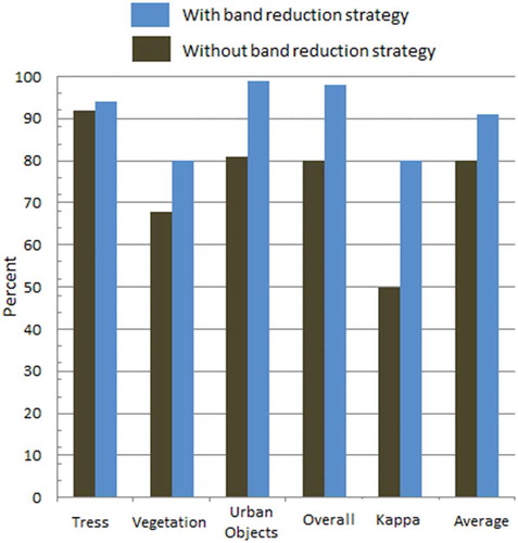
Furthermore, the effect of the band reduction strategy on the produced textural features was assessed. For this purpose, first three bands of the visible image and five bands of the MNF output were fed to the classifier and second, the classification was applied without using band reduction strategy. The obtained results for overall, average, class accuracies and Kappa coefficient values were compared in Figure 4. The gained results show the efficiency and importance of the band reduction strategy on the noisy and correlated bands for increasing classification accuracy while there were enough training samples and are unlike to Hughes phenomenon (Hughes, 1968). The overall accuracy, average accuracy and Kappa coefficient values improved approximately 17%, 12% and 30%, respectively, while “trees” class accuracy improved 2%, the vegetation and urban objects classes’ accuracies increased about 13% and 17%, correspondingly, by using band reduction strategy.

Figure 4. Importance of band reduction strategy on the noisy and correlated bands.

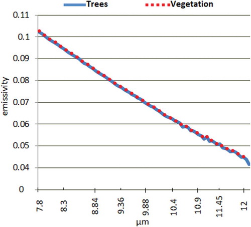
Hyperspectral data with an enormous number of contiguous spectral bands have been applied to discriminate the materials that typically cannot be separated by multiband RS data (Chang, 2003). In this research for the first time, HTIR with very high spatial and spectral resolution was evaluated for discrimination of two vegetation types: trees and vegetation classes. In Figure 5, radiation versus wavelength spectral signatures of trees and vegetation classes were shown. It is obvious that the spectral signatures of the trees and vegetation classes have behaved similarly in the 84 spectral bands of the HSR-HTIR data. So using HSR-HTIR data for discrimination of vegetation types, particularly trees and vegetation classes, will descend the classification accuracy.

Figure 5. Spectral curves of the tress and vegetation classes for HTIR.

Second step: bare soil, roofs and roads mapping

As mentioned before the proposed method in this paper consists of three main steps. In the second step, TIR and visible data were combined for mapping the bare soil, roads and (red, concrete, gray) roof buildings classes. Therefore, after atmospheric correction of TIR data by in-scene atmospheric compensation approach, SPPP band reduction method adapted on the HSR-HTIR data and nine spectral TIR bands were estimated (see Figure 6(a)). In the next phase similar to the visible image, six textural features were extracted from TIR data, which consist of entropy, variance, ASM, mean, homogeneity and dissimilarity. For every bands of TIR image, all mentioned textural features were estimated in four directions (0°, 45°, 90° and 135°). Then, the average of the four direction bands was estimated.

Figure 6. TIR band reduced (a), first MNF band on TIR (b) and final classification map for second step (c).

Next, MNF band reduction approach was applied to the outcome of those 56 bands and five first bands were selected (see Figure 6(b)). Finally, nine spectral and five textural bands of TIR data combined with three spectral and five textural bands of the visible image and were fed to an SVM classifier. The result of this step was the six mapped urban land cover classes, which was shown in Figure 6(c).

In Table 3 the error matrix for the results of the proposed method in the second step is shown. In Table 3, achieved results of the second step were compared with two other situations. In the first situation, we used only spectral and textural features of the visible image for discrimination of the six considered classes of the second step. In the second one, we combined spectral and textural features of the visible image with spectral features of TIR data to discriminate six considered classes. According to the results of Table 3, using spectral and textural features of TIR data increased the overall accuracy and Kappa coefficient value of the second step about 92.01% and 0.885, respectively. Moreover, the overall accuracy and Kappa coefficient value of the using only spectral and textural features of the visible image combined with spectral bands of TIR data were 85.55% and 0.79, correspondingly.

Table 3. Error matrix for step (2), using only visible bands and visible bands combined with only spectral bands of TIR.

		Actual class
	Method	Class name	Roads	Urban vegetation	Red roof	Gray roof	Concrete roof	Bare soil
Predicted class	Step (2)	Roads	93.26	1.79	0.13	7.72	1.54	0.80
		Urban vegetation	0.01	96.24	0.01	0.97	0.08	3.05
		Red roof	0.54	1.15	93.62	2.86	0.04	9.64
		Gray roof	4.80	0.75	5.70	86.28	8.91	0.02
		Con roof	1.38	0.04	0.34	2.17	89.42	0/21
		Bare soil	0.01	0.02	0.20	0	0	86.26
	Visible Spectral–textural and TIR Spectral	Roads	81	0	0.44	2.41	0.74	0
		Urban vegetation	0	93.68	0.11	0.95	0	0.53
		Red roof	0.36	3.52	92.18	3.02	0.08	22.14
		Gray roof	13.71	2.27	6.92	92.70	7.73	0.90
		Con roof	4.93	0	0.26	0.92	91.45	0
		Bare soil	0	0.02	0.10	0	0.01	76.42
	Visible Spectral–textural	Roads	66.62	0	0.97	7.44	0.12	0
		Urban vegetation	0.01	96.17	0.02	0.97	0	0.36
		Red roof	0.83	0.48	91.44	1.29	0.11	20.13
		Gray roof	27.60	2.52	7.16	89.42	8.66	0.14
		Con roof	4.93	0	0.29	0.88	91.10	0
		Bare soil	0.01	0.91	0.11	0	0	79.37

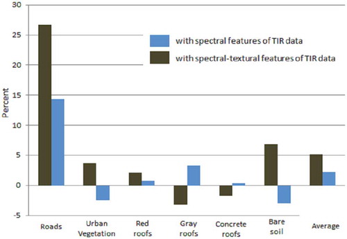
ULCM overall accuracy and Kappa coefficient value for employing only spectral bands of the visible image were 77.60% and 0.69, respectively. The efficiency of the TIR data for increasing the ULCM accuracy was shown by the obtained results. The highest classes’ accuracies were reached by the “roads”, “urban vegetation” and “red roofs” classes by the proposed strategy in second step. “Gray” and “Concrete” roof classes have their best accuracy in the situation in which spectral and textural features of the visible image combined with TIR spectral data. Further, in Figure 7, class accuracy and average accuracy increasing for using spectral and spectral–textural features of TIR were compared.

Figure 7. TIR spectral and textural features influence on the class accuracy increase.

HSR TIR, a novel source of RS data, was not studied for urban object detection. In this research for evaluation of the enactment of this data on ULCM applications, nine spectral bands of TIR were fed to SVM classification method. Obtained results were shown as error matrix in Table 4 for six desired classes: “roads”, “(gray, red, concrete) roof buildings”, “bare soil” and “urban vegetation”.

Table 4. Error matrix for classification based on TIR spectral bands.

	Actual class
Predicted class	Class name	Roads	Urban vegetation	Red Roof	Gray Roof	Concrete Roof	Bare soil
	Roads	90.60	3.22	10.52	5.97	6.36	1.33
	Urban vegetation	1.85	44.35	2.71	3.49	40.46	46.45
	Red roof	0.57	1.41	38.91	37.47	12.23	0.80
	Gray roof	2.78	8.99	39.37	44.67	16.74	1.23
	Con roof	4.13	42	8.38	8.33	23.52	34.19
	Bare soil	0.07	0.03	0.11	0.07	0.70	16.00
	Total	100	100	100	100	100	100

Achieved results have shown overall accuracy, average accuracy and Kappa coefficient values about 67.36%, 43% and 0.499, correspondingly. According to the results of Table 3 (i.e. last part of Table 3) and Table 4, in the case of employing just spectral bands of visible image, “bare soil” and “red building” classes are classified in a less accuracy. Whereas, by fusing spectral and textural bands of the TIR with the visible image features, these classes are classified with an acceptable accuracy. Also, “roads” class discriminated impeccably by using TIR spectral bands, while in the case of employing spectral and textural features of the just visible there was correlation between “roads” and “gray roof building” classes, and it shows the efficiency of the TIR data.

Furthermore, except roads class, other urban classes’ accuracies were under 50%, and the obtained results have shown the important points about the performance of TIR spectral bands in ULCM applications. Moreover, “urban vegetation” class detection in the case of using visible features has more acceptable results in comparison to the using TIR spectral and textural bands.

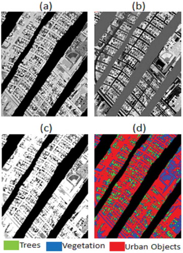
Third step, map combination

In third step, the produced maps in the first and second step were combined. The combined map was a raw classified map which consists of the all seven desired classes (see Figure 8(a)). In the third step, the effectiveness of ORBPP method applied to the raw classified map and final ULCM was produced (see Figure 8(b)) (Eslami et al., 2015).

Figure 8. Final map before post-processing (a) and after post-processing (b).

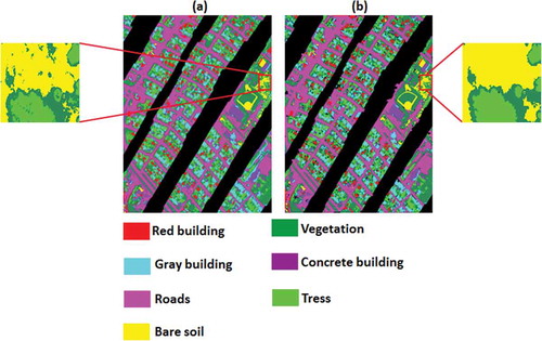
The error matrix for the final map is shown in Table 5. The final map has Kappa coefficient value of 0.928, overall accuracy of 94.96% and average accuracy of 93.62%. According to Table 5 and discussed contents, “vegetation” class has correlation only with “trees” class. The maximum class accuracy occurred for the roads class was about 97.66%, which happened because of the influence of the TIR data in the classification results. Likewise, the minimum class accuracy happened to the “gray roof building” class because of the high correlation between roads and gray roof building in the TIR data. Because of using TIR spectral and textural features in the proposed method, the correlation between bare soil and red roof building classes was the least value.

Table 5. Error matrix for final ULCM map.

	Actual class
Predicted class	Class name	Roads	Vegetation	Red Roof	Gray Roof	Concrete Roof	Bare soil	Trees
	Roads	97.66	0	0.03	5.20	1.51	1.85	0
	Vegetation	0.01	93.12	0.11	0.99	0.55	3.62	4.86
	Red roof	0.32	0	94.01	2.03	0	0	0
	Gray roof	1.50	0	5.63	90.13	7.12	0	0.03
	Con roof	0.50	0	0	1.65	90.82	0	0.02
	Bare soil	0.01	0	0.20	0	0	94.53	0
	Trees	0	6.88	0.03	0	0	0	95.10
	Total	100	100	100	100	100	100	100

Furthermore, the final Kappa coefficient value and overall accuracy were compared with the best results of the Data Fusion Contest 2014 which was announced by IEEE GRSS (see Table 6). The obtained results showed the efficiency of the proposed method, which was just used textural and spectral features, while in the previous works they used other spatial features of visible image for classification. Furthermore, the adopted results showed the undeniable influence of the using two newly proposed VIs and for the first time the influence of textural features of the TIR data in increasing the ULCM final map accuracy, while in the previous works nobody has evaluated the influence of the textural features of the TIR data for ULCM final map production.

Table 6. The results of the IEEE Data Fusion Contest 2014 and proposed method.

Rank	Researchers	Kappa coefficient value	Overall accuracy (%)
1	Xin. H et al. (Liao et al., 2015)	0.9438	96.31
2	Eslami and Mohammadzadeh	0.9283	94.96
3	Weng. C et al. (Liao et al., 2015)	0.9217	–
4	Li. J et al. (Liao et al., 2015)	0.9120	–
5	Eslami and Mohammadzadeh (Eslami et al., 2015)	0.9043	92.63
6	Sridharan. H et al. (Liao et al., 2015)	0.9039	–
7	Guan. X et al. (Liao et al., 2015)	0.90	–
8	Zhong. Y et al. (Liao et al., 2015)	0.892	–
9	Kang. X et al. (Liao et al., 2015)	0.8917	–
10	Lee. L et al. (Liao et al., 2015)	0.8894	–

Conclusion

In this study, a comprehensive novel method was proposed for ULCM by fusion of the textural and spectral features of HSR visible and TIR data. The method consisted of three main steps. In the first step, spatial and spectral features of just visible image were used for discrimination of the “trees” and “vegetation” classes, while two new VIs – SVI and MSVI – were introduced and tested. Obtained results underlined the effectiveness of two newly proposed VIs compared with the best results of the well-known VIs. Also, the result assessment has shown the important performance of the proposed approach in the first step for the separation of “trees” and “vegetation” classes. In the second step, for the first time, textural and spectral features of the visible and TIR data were fused for the detection of “roads, buildings” (with different roofs) and “bare soil” classes. Achieved results have revealed the significant influence of the textural features of the TIR for increasing the ULCM accuracy. In the third step, the outcomes of the first and second steps were combined and built the final raw classification map. Then, the achieved raw map was fed to a post-processing approach and final map was produced. Attained results showed that using TIR textural features increased the overall accuracy and Kappa coefficient value about 7% and 9%, respectively. Also, gained outputs from complete analyses of the “vegetation” and “trees” classes’ spectral signatures on the HTIR data have demonstrated the same behavior of these classes on the HSR-HTIR data. Furthermore, in this study the spectral bands of HSR-TIR data were fed to an SVM classifier and considered urban objects were classified. Achieved results showed that “roads” class was detected by TIR data more accurately, while other ones have the class accuracy less than 50%. Moreover, the ULCM results were compared constructively with the best results of the Data Fusion Contest 2014 announced by IEEE GRSS and its efficiency was revealed. For future works, more spatial features of the TIR data will be examined for improvement of accuracy.

Acknowledgment

The authors thank Telops Inc. (Québec, Canada) for providing the data set that was used in this article. The authors like to thank the IEEE GRSS IADF Technical Committee for providing us the data access of the Data Fusion Contest 2014.

Disclosure statement

No potential conflict of interest was reported by the authors.

References

- Aguilar, M.A., Fernández, A., Aguilar, F.J., Bianconi, F., & Lorca, A.G. (2016). Classification of urban areas from GeoEye-1 imagery through texture features based on histograms of equivalent patterns. European Journal of Remote Sensing, 49, 93–331. doi:10.5721/EuJRS20164906
- Albregtsen, F. (2008). Statistical texture measures computed from gray level co-occurrence matrices. In Image processing laboratory, Department of Informatics, University of Oslo (pp. 1–14).
- Amato, U., Cavalli, R.M., Palombo, A., Pignatti, S., & Santini, F. (2009). Experimental approach to the selection of the components in the minimum noise fraction. IEEE Transactions on Geoscience and Remote Sensing, 47(1), 153–160. doi:10.1109/TGRS.2008.2002953
- Bannari, A., Morin, D., Bonn, F., & Huete, A. (1995). A review of vegetation indices. Remote Sensing Reviews, 13(1–2), 95–120. doi:10.1080/02757259509532298
- Benediktsson, J.A., Pesaresi, M., & Amason, K. (2003). Classification and feature extraction for remote sensing images from urban areas based on morphological transformations. IEEE Transactions on Geoscience and Remote Sensing, 41(9), 1940–1949. doi:10.1109/TGRS.2003.814625
- Bovolo, F., Camps-Valls, G., & Bruzzone, L. (2007). An unsupervised support vector method for change detection. In Remote Sensing (pp. 674809-674809). International Society for Optics and Photonics.
- Brook, A., Vandewal, M., & Ben-Dor, E. (2012). Fusion of optical and thermal imagery and lidar data for application to 3-d urban environment and structure monitoring. In Escalante-ramirez, B. Remote sensing-advanced techniques and platforms: Chengdu,China, InTech (pp. 29–50).
- Burges, C.J. (1998). A tutorial on support vector machines for pattern recognition. Data Mining and Knowledge Discovery, 2(2), 121–167. doi:10.1023/A:1009715923555
- Chang, C.-I. (2003). Hyperspectral imaging: Techniques for spectral detection and classification (Vol. 1). Springer Science & Business Media.
- Cockx, K., Van de Voorde, T., & Canters, F. (2014). Quantifying uncertainty in remote sensing-based urban land-use mapping. International Journal of Applied Earth Observation and Geoinformation, 31, 154–166. doi:10.1016/j.jag.2014.03.016
- Eslami, M., & Mohammadzadeh, A. (2016). Developing a Spectral-Based Strategy for Urban Object Detection From Airborne Hyperspectral TIR and Visible Data. IEEE Journal of Selected Topics in Applied Earth Observations and Remote Sensing, 9(5), 1808-1816.
- Geman, S., & Geman, D. (1984). Stochastic relaxation, Gibbs distributions, and the Bayesian restoration of images. IEEE Transactions on Pattern Analysis and Machine Intelligence, (6), 721–741.
- Gitelson, A.A. (2004). Wide dynamic range vegetation index for remote quantification of biophysical characteristics of vegetation. Journal of Plant Physiology, 161(2), 165–173.
- Gitelson, A.A., Kaufman, Y.J., Stark, R., & Rundquist, D. (2002). Novel algorithms for remote estimation of vegetation fraction. Remote Sensing of Environment, 80(1), 76–87.
- Green, A.A., Berman, M., Switzer, P., & Craig, M.D. (1988). A transformation for ordering multispectral data in terms of image quality with implications for noise removal. IEEE Transactions on Geoscience and Remote Sensing, 26(1), 65–74.
- Guo, L., Chehata, N., Mallet, C., & Boukir, S. (2011). Relevance of airborne lidar and multispectral image data for urban scene classification using random forests. ISPRS Journal of Photogrammetry and Remote Sensing, 66(1), 56–66.
- Haralick, R.M., & Shanmugam, K., (1973). Textural features for image classification. IEEE Transactions on Systems, Man and Cybernetics, 3(6), 610–621.
- Hughes, G.P. (1968). On the mean accuracy of statistical pattern recognizers. IEEE Transactions on Information Theory, 14(1), 55–63.
- Knipling, E.B. (1970). Physical and physiological basis for the reflectance of visible and near-infrared radiation from vegetation. Remote Sensing of Environment, 1(3), 155–159.
- Kuenzer, C., & Dech, S. (2013). Thermal infrared remote sensing. In Sensors, Methods, Applications, Remote Sensing and Digital Image Processing (Vol. 17). Springer Netherlands.
- Liao, W., Huang, X., Van Coillie, F., Gautama, S., Pizurica, A., Philips, W., ... & Tuia, D. (2015). Processing of multiresolution thermal hyperspectral and digital color data: Outcome of the 2014 IEEE GRSS Data Fusion Contest. IEEE Journal of Selected Topics in Applied Earth Observations and Remote Sensing, 8(6), 2984-2996.
- Lin, H.-D., & Bruce, L.M. (2003). Parametric projection pursuit for dimensionality reduction of hyperspectral data. In Paper presented at the geoscience and remote sensing symposium, 2003. IGARSS’03. Proceedings. IEEE International Geoscience and Remote Sensing Symposium (IGARSS). Vol. 6, pp. 3483-3485.
- Lopes, A.P., Nelson, B.W., Graça, P.M., Wu, J., Tavares, J.V., Prohaska, N., et al. (2015). Band combinations for detecting leaf amount and leaf age in QuickBird satellite and RGB camera images. Brazilian Remote Sensing Symposium. Vol. (17), pp. 1671-1677.
- Mohammadzadeh, A., Zoej, M.V., & Tavakoli, A. (2008). Automatic main road extraction from high resolution satellite imageries by means of self-learning Fuzzy-GA algorithm. Journal of Applied Sciences, 8(19), 3431–3438.
- Mountrakis, G., Im, J., & Ogole, C. (2011). Support vector machines in remote sensing: A review. ISPRS Journal of Photogrammetry and Remote Sensing, 66(3), 247–259.
- Patra, S., Modi, P., & Bruzzone, L. (2015). Hyperspectral band selection based on rough set. IEEE Transactions on Geoscience and Remote Sensing, 53(10), 5495–5503.
- Prakash, A. (2000). Thermal remote sensing: Concepts, issues and applications. International Archives of Photogrammetry and Remote Sensing, 33(B1; PART 1), 239–243.
- Richards, J.A., & Richards, J. (1999). Remote sensing digital image analysis (Vol. 3), 4th Edition. Berlin: Springer.
- Rottensteiner, F., Sohn, G., Gerke, M., Wegner, J.D., Breitkopf, U., & Jung, J. (2014). Results of the ISPRS benchmark on urban object detection and 3D building reconstruction. ISPRS Journal of Photogrammetry and Remote Sensing, 93, 256–271.
- Sarp, G., Erener, A., Duzgun, S., & Sahin, K. (2014). An approach for detection of buildings and changes in buildings using orthophotos and point clouds: A case study of Van Erciş earthquake. European Journal of Remote Sensing, 47, 627–642.
- Soh, L.-K., & Tsatsoulis, C. (1999). Texture analysis of SAR sea ice imagery using gray level co-occurrence matrices. IEEE Transactions on Geoscience and Remote Sensing, 37(2), 780–795.
- Theodoridis, S., Pikrakis, A., Koutroumbas, K., & Cavouras, D. (2010). Introduction to pattern recognition: A matlab approach. USA: Academic Press imprint of Elsevier.
- Uzar, M. (2014). Automatic building extraction with multi-sensor data using rule-based classification. European Journal of Remote Sensing, 47(8), 1–18.