Land cover classification in Romanian Carpathians and Subcarpathians using multi-date Sentinel-2 remote sensing imagery

ABSTRACT

In this article, we processed Sentinel-2 images in order to obtain high accuracy land cover maps for two complementary study areas. The first is represented by the Romanian Subcarpathians, a hilly highly fragmented area with heterogeneous land cover pattern and the second by Romanian Carpathians, a mountain area with homogenous structure of vegetation cover. The aim of this article is to evaluate the potential of a singledate in comparison with multi-date images for which a complete calibration and an iterative process of supervised classification using Maximum Likelihood (ML) and Support Vector Machine (SVM) algorithms were applied for the both study areas. The results show that in the case of Subcarpathian area, the SVM classification on multi-date images has better accuracy due to high complexity of the land cover pattern and spectral similarities between classes, while in the Carpathians, the ML returns good accuracy, consequence of high spectral separabilities between compact features. The validation process based on ground reference data shows good accuracies, about 92.41% for the Subcarpathians and 98.65% for the Carpathians. It is clearly noticed that the land cover pattern determines the use of different algorithms and the multi-date images enhance the overall accuracy of the classification.

KEYWORDS:

• Sentinel-2
• land cover
• multi-date images
• supervised classification
• support vector machine
• maximum likelihood

Introduction

Land cover maps still remain one of the first products from remote sensing image analysis in Earth Observation application projects (Chuvieco, 2016). Since the end of the 1970s and 1980s, the US Geological Survey Land Use Land Cover Classification system (Anderson, Hardy, Roach, & Witmer, 1976) and later the European Environmental Agency’s Corine Land Cover (Büttner, Feranec, & Jaffrain, 2000) vector data (1990–2012) provided the first data coverage at National and Continental levels, based on the interpretation of different available imagery (Landsat, IRS, SPOT etc.). Food and Agriculture Organization of the United Nations started in 1990 the development of the Land Cover Classification System (LCCS), first evaluated in Africa (Di Gregorio & Jansen, 1997), and later implemented as a software platform in 2000, LCCS(v1) (Di Gregorio & Jansen, 2000). LCCS and the Land Cover Meta-Language were adopted as standards in 2009 and 2012 (ISO-19144-1, 2009; ISO-19144-2, 2012). There can also be mentioned the Global level land cover databases, as GLC-SHARE (Latham, Cumani, Rosati, & Bloise, 2014), GlobeLand30 (Chen et al., 2015), GlobCover (Arino et al., 2008) and GLC2000 (Bartholomé & Belward, 2005; Hansen, Defries, Townshend, & Sohlberg, 2000).

Land cover was also the subject of many scientific approaches, including change detection analysis at different scales, from European to National levels. (Feranec, Hazeu, Christensen, & Jaffrain, 2007; Feranec, Hazeu, Jaffrain, & Cebecauer, 2007; Feranec, Jaffrain, Soukup, & Hazeu, 2010)

Remote sensing data selection for land cover mapping need to be adapted to the objectives of mapping and to the study area features (Campbell & Wynne, 2011; Robin, 1998). Romanian Carpathians and Subcarpathians landscapes feature a complex land cover pattern, with an average minimum mapping unit which cannot be reached with medium resolution imagery like Landsat Operational Land Imager (OLI) (Rujoiu-Mare & Mihai, 2016).

The recently available Sentinel-2 MultiSpectral Instrument (MSI) imagery represents a new opportunity in finer scale land cover mapping, especially for the most complex landscapes, with higher degree of fragmentation. It is the typical case of Romanian Carpathians and Subcarpathians, with a diversified landscape pattern, introduced by a high anthropogenic transformation of the primary land cover: forest fragmentation, deforestation, intensive grazing, fragmented pattern of agricultural plots around villages and town built-up areas. The 13 spectral bands of Sentinel-2 MSI sensor with fine spatial resolution (10, 20, 60 m) (Drusch et al., 2012) and spectral resolution and several near-infrared wavelength intervals (Delegido, Verrelst, Alonso, & Moreno, 2011) enable an advanced image analysis and land cover mapping at local levels.

The aim of our article is to evaluate available Sentinel-2 MSI imagery in mapping land cover at local scale, after the complete calibration of the data sets from complementary areas: Prahova Subcarpathians, a hilly area with a highly complex land cover pattern, fragmented by valley corridors (about 200–1100 m a.s.l. – above sea level) and Bucegi Massif (700–2500 m a.s.l.), featuring all the main vegetation zones in the Carpathians and an intensive anthropogenic influence by traffic and tourism.

The second objective of our study is to evaluate the use of multi-date images for the classification in order to be able to distinguish the land cover features with similar spectral response and to decrease the classification errors. Old land cover maps generated from a single-date image have low thematic accuracies, especially where the feature classes were complex and heterogeneous. This technique of using multi-date images in classification was used and assessed in many recent studies (Parmentier & Eastman, 2014; Sexton, Urban, Donohue, & Song, 2013; Shao, Lunetta, Wheeler, Iiames, & Campbell, 2016), and it had been demonstrated that maps generated using temporal series approaches have higher accuracies than using single image methods (Gomez, White, & Wulder, 2016; Khatami, Mountrakis, & Stehman, 2016). The two main factors that influence the classification accuracy and that can be controlled by the analyst are the input data and the classification algorithm (Khatami et al., 2016). The multi-date imagery could be defined as the use of multiple images for a single classification images (Khatami et al., 2016). Using multi-date images in classification instead of single-date data, multiple spectral variables are captured and used for an optimal detection and discrimination between the land cover types. Furthermore, it has been demonstrated that including multiple spectro-temporal variables in the analysis improves the classification overall accuracy with 6.9% (Khatami et al., 2016) and also increases the feature space (Gomez et al., 2016). We applied this technique to different areas with various complexities, in order to produce a single-date land cover map from multiple observations acquired within a year.

Materials and methods

Study areas

For this study, we have chosen two areas from Romanian Subcarpathians and Carpathians. These regions have different land cover features, and for this reason, it was necessary to use distinct algorithms and processing techniques for classifying the images.

The Subcarpathian region between Prahova (West) and Teleajen (East) Valleys is limited by the Ploiești piedmont Plain on the southern part and Baiu and Grohotiș Mountains on the northern part (Figure 1). The average altitude of this area is about 616 m, ranging from 185 to 1047 m (Vârful Frumos Peak). It is characterized by complex and different land cover features with natural processes, such as erosion and landslides, and also by human activities, including quarries, mining and oil gas platforms from the last 200 years. This complex of heterogeneous land cover features often generates errors in classifications because of the spectral similarities of some classes, as well as bare land, built-up areas and croplands or deciduous forest and sparsely vegetated areas.

Figure 1. Location map of the study areas.

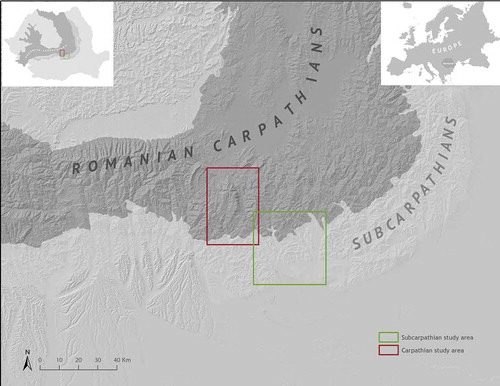
Bucegi Mountains are situated in the Southern Carpathians, West from Prahova Valley (Figure 1). The altitude of the massif varies from 700 to 2505 m (Omu Peak), with rocky abrupt and suspended plateaus, assuring high biodiversity (Sârbu et al., 2013) on its slopes. It includes a Natural Park designated as V IUCN category, for protecting fir and spruce forests, associated with subalpine grassland and high specific biodiversity of flora and fauna. The area is characterized by a complex land cover on the plateau, with buildings, roads and erosional areas, but relatively homogenous in forest areas.

Data sets used in the analysis

For this analysis, we have used multiple clouds-free and snow-free Sentinel-2 imagery from different months over a year period (Table 1). All the granules used for both study sites were included in the same Sentinel-2 scene product. We integrated different ancillary data for enhancing the satellite images, for validating the classifications and for mapping the results (Figure 2).

Table 1. Data sets and data sources used in the analysis.

Data sets	Spatial resolution /scale	Date of acquisition	Source
Sentinel-2 satellite images	10, 20, 60 m	8 August 201528 August 201523 December 20154 April 201613 July 2016	Global Monitoring for Environment and Security (GMES) – Copernicus
Elevation DEM	10 m	1981	Contours from Topographic Military Maps 1:25 000, Military Mapping Directorate
Orthophotos	0.5 m	2012	National Agency for Cadastre and Land Registration (ANCPI, Bucharest, Romania)

Figure 2. The workflow of the analysis.

Comparing with Landsat 8 OLI data (Table 2), each granule of Sentinel-2A product covers 100 km² and contains 13 spectral bands. The temporal resolution of Sentinel-2 images is 10 days now, but it will increase up to 5 days, when Sentinel-2B MSI sensor will be active (Wulder et al., 2015). The new bands around the red-edge region at 20 m spatial resolution, centred at 705, 740, 783 and 865 nm, are very useful for vegetation discrimination and land cover production (Delegido et al., 2011).

Table 2. Comparison between Sentinel-2A MSI (ESA, 2015) and Landsat 8 OLI bands (USGS, 2016).

Sentinel-2A MSI data				Landsat 8 OLI data
Band number	Band name	Spatial resolution	Central wavelengths (nm)	Band number	Spatial resolution	Central wavelengths (nm)
B1	Coastal/aerosols	60 m	443	B1	30 m	443
B2	Visible Blue	10 m	490	B2	30 m	482
B3	Visible Green	10 m	560	B3	30 m	561
B4	Visible Red	10 m	665	B4	30 m	654
B5	NIR 2	20 m	705	–	–	–
B6	NIR 3	20 m	740	–	–	–
B7	NIR 4	20 m	783	–	–	–
B8	NIR 1	10 m	842	B5	30 m	864
B8A	NIR 5	20 m	865	–	–	–
B9	Atmospheric /water vapour	60 m	945	–	–	–
B10	Cirrus	60 m	1375	B9	30 m	1 373
B11	SWIR 1	20 m	1610	B6	30 m	1608
B12	SWIR 2	20 m	2190	B7	30 m	2200

Images pre-processing techniques

The Sentinel-2 data, level 1C available for download are geometrically and radiometrically corrected images, containing Top of the Atmosphere reflectances in cartographic geometry (UTM projection, WGS 84 datum). For land cover classification production, calibrated data in terms of topographic ground reflectance are needed. For this reason, it is important to apply atmospheric and illumination corrections on the L1C images.

Atmospherically corrected data were obtained using the Sen2Cor plugin available on SNAP software. This application depends on the calculation of the radiative transfer functions for different sensors and solar geometries, ground elevations and atmospheric parameters (Müller-Wilm, 2015). It is based on the libRadtran library (Mayer & Kylling, 2005), which contains the calculations of solar and thermal radiation on the Earth’s atmosphere. This library generates the Look-up Tables necessary for the processor to read the parameters (Müller-Wilm, 2015) for each sequential band.

The Top of the Atmosphere reflectance L1C input images was transformed in the Bottom of the Atmosphere reflectance at L2A processing level, including the Surface Reflectance bands, resampled and generated for an equal resolution (10 m), an Atmospheric Optical Thickness (AOT) image and a Water Vapour map (WV). The AOT and WV images were calculated with the help of the Coastal /Aerosols band (B1) and Atmospheric/Water Vapour band (B9). The band 10 (Cirrrus) is omitted from the L2A output as it does not contain surface information (Müller-Wilm, 2015).

For the illumination corrections of the images, we have used the C-correction formula, proposed by Teillet, Guindon, and Goodenough (1982) in order to remove the shadows effects on the image and to unify the spectral response of the similar land cover features.

)

where

ρ_λ,h,i = surface reflectance, topographically corrected bands

ρ_λ,i = surface reflectance of the spectral bands

= solar zenith angle (in radians)

γ_i = illumination angle (in radians)

c_λ = empirical constant for each band (generated from linear regression plot between the illumination angle and each spectral band).

This algorithm needs the solar zenith angle, available in the metadata file and a digital model of elevation co-registered with the images to be corrected (the same cover extent, spatial resolution, geometries references and correlation between pixels). For this reason, we used the contour lines extracted from Military Topographic Map (1:25 000, with 5 m equidistance) in order to create a digital elevation model (DEM) at 10 m spatial resolution. Using the DEM and the sun azimuth and sun elevation angles for the Sentinel-2 images, we generated the angle of incidence, which is complementary to the angle of illumination (Hantson & Chuvieco, 2011; Riano, Chuvieco, Salas, & Aguado, 2003; Vanonckelen, Lhermitte, & Van Rompaey, 2013).

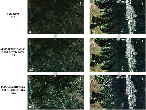
These atmospheric and illumination corrections were applied on each multi-date granules used in the analysis for the both study areas of Bucegi and Prahova-Teleajen Subcarpathians. Thus, the new resulted images at L2A level of processing contain topographic corrected surface reflectances (Figure 3).

Figure 3. Calibration workflow results of the Sentinel-2 images for Prahova-Teleajen Subcarpathians (A) and Bucegi Mountains (B).

Training sample collection and evaluation

The supervised classification process starts with training areas creation for each land cover class from the study areas. Being a fragmented territory, the Subcarpathian area contains more land cover classes than the mountainous region, presented in Table 3.

Table 3. Land cover classes for each study area and their description.

	Land cover classes		Description
	Prahova-Teleajen Subcarpathians (number of ROI pixels)	Bucegi Mountains (number of ROI pixels)
1	Coniferous forest (750)	Coniferous forest (324)	Abies alba, Picea abies, Pinus sylvestris, Larix decidua, Pinus cembra
2	Deciduous forest (3080)	Deciduous forest (144)	Fagus sylvatica, Querqus petraea, Querqus robur, Robinia Pseudacacia
3	–	Dwarf pine (356)	Pinus mugo
4	–	Mixed forest (208)	Picea abies, Abies alba and Fagus sylvatica
5	Sparsely vegetated areas (including orchards and shrubs) (264)	–	Orchards, shrubs and different broadleaves species with rare densities grown close to settlements and roads
6	Grasslands (3714)	Grasslands (304)	Herbaceous area used for pastures or hays
7	Croplands (1518)	–	Agricultural lands (cereals or vegetables) cultivated in the depressions or at the contact with the plain (South from Subcarpathian area)
8	Built-up area (950)	–	Settlements, transport and hydrotechnical facilities, industry
9	Bare land (961)	–	Mainly riverbeds, but also bare soil and bare rock
10	–	Bare land/built-up area (80)	Constructions, roads, tracks, as well as bare soil/rock or degraded grassland
11	Water bodies (1153)	Water bodies (208)	Reservoirs, lakes and rivers

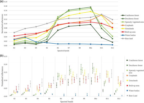
The training areas were statistically validated in correlation with the associated input data. Firstly, we computed a series of graphs showing the mean spectral signature (Figure 4a) and the standard deviation (Figure 4b) for each land cover class in every spectral band from the input image. These graphs evaluate the spectral separability between the training areas to see if they are statistically different. The smallest standard deviation bars from the spectral dispersion graph (Figure 4b) show that the reflectances within a region of interest (ROI) class in a spectral band are similar. The largest ones reflect a lot of variability in the spectral reflectance characteristics of a ROI class. The error bars of two or more ROI classes that overlap show spectral similarities between those classes and potential errors generated in the classification.

Figure 4. Evaluation of the spectral separability between the training areas for a single-date image from 28 August 2015, Subcarpathian area: (a) spectral signature plot; (b) spectral dispersion graph.

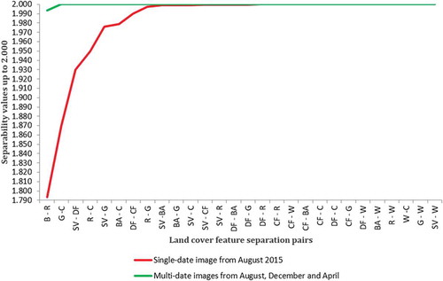
Secondly, we calculated the ROI spectral separability using the Jeffries–Matusita and Transformed Divergences algorithms. These techniques showed how well separated were the land cover classes, comparing them in pairs. These algorithms for quantitative expressions of the ROI separability are based on the covariance and weighted distance between the mean values of the classes (Chuvieco, 2016). The result is a table showing the statistics separability of pairs. The highest value is 2000 and it shows that those classes are clearly separated on the input image (the weighted distance between classes is high). The values lower than 2.00 indicate that confusions between the land cover classes and these errors will be propagated in the classification.

For improving the separability between the land cover classes, we added more spectral bands as input data for the classification. For the Subcarpathian area, we have used three intra-annual Sentinel-2 scenes, from different vegetation seasons (summer, winter and spring), in order to eliminate the confusions between the land cover classes and distinguish the spectral response. Using multi-date images in the classification generates changes in the training samples data, which collects a large spectral variability (Sexton et al., 2013). Thereby, the training sets include various spectral signatures of the land cover classes captured across time and space.

For Bucegi Mountains, we have used two granules for the classification because the land cover classes are more compact and clearly separated. Both selected images were from the summer season, for as there were no clouds-free or no snow-free images available from the other seasons for the mountainous area.

Multi-date image classifications

Choosing the right classification algorithm is also a difficult task because of the land cover classes and their spectral signatures. maximum likelihood (ML) is a parametric widely used algorithm and it evaluates the variance and covariance of the spectral response for each class (Chuvieco, 2016). It computes the probability of each pixel value to belong to each land cover classes and assigns it to the class with the high probability value (Chuvieco, 2016; Lillesand, Kiefer, & Chipman, 2015; Schowengerdt, 2007). This algorithm manages well with compact land cover classes, but there are necessary large and pure training samples (Gomez et al., 2016). It returns good results on the mountainous area where the land cover classes are more compact and homogeneous, but in the Subcarpathian region, it generates lots of confusions between built-up area, bare land and croplands or deciduous forests and sparsely vegetated areas class.

Support vector machine (SVM) is a non-parametric classification algorithm that yields good results from complex and noisy data (Chuvieco, 2016) because it separates the land cover categories using a decision surface that maximizes the margins of the classes (M. Hansen, 2012) and the spectral response of the classes does not over-fit (Gomez et al., 2016). It manages well large feature space, and there are not necessary large training samples, but they need to contain a wide range of spectral variability of the classes (Gomez et al., 2016). It includes a penalty parameter that controls the margins between classes where the training data are non-separable, allowing a certain degree of misclassification. This algorithm was tested on various feature space, compared with other classification algorithms as ML and neural networks and it returned good results with lower errors (Khatami et al., 2016).

Both algorithms were applied for each study area and the best results were selected for further processing and analysis. As mentioned earlier, the SVM managed well the heterogeneous classes of the Subcarpathians, while the ML classified well the compact land cover structure.

Accuracy assessments of the classification results

Each classification was assessed with a set of ground truth collected on the orthophotos (2012) and from field observations, for both study areas. For the Subcarpathian region, we used 11,206 sample points with a near-uniform spatial distribution and an average density of 7.6 points per square kilometre. For the Carpathian region, we used 446 sample points with an average density of 7.5 points per square kilometre. The confusion matrices were computed to compare the relationship between the known reference data and the results from the classifications (Lillesand et al., 2015). These methods show the overall accuracies, kappa coefficients and the various errors of commission and omission related to user’s and producer’s accuracies.

Results

The spectral signature plot (Figure 4a) for a single-date image from 28 August 2015 for Subcarpathian area shows overlaps for deciduous forest with sparsely vegetated and built-up areas with croplands. The spectral dispersion graph for the same image shows the variance in the reflectances of each category. Deciduous, coniferous and sparsely vegetated areas have low error bars in the visible spectrum; therefore, the spectral signatures of each category are similar. Otherwise, in red edge bands, near-infrared and short-wave infrared spectrum, the error bars for deciduous, coniferous and sparsely vegetated areas show a high spectral variability in the spectral signatures. The built-up area and bare land have high variability in the visible spectrum. On the other hand, the error bars of build-up area and croplands are overlapping which means that those classes are not statistically different and they will be mismatched in the classification process. The same problems appear between deciduous forest and sparsely vegetated area classes and for bare land with croplands and built-up area.

For improving the spectral separability between land cover classes, we used multi-date images as input data. The results of the separability of the training areas (Figure 5) associated with multi-date images were increased, the lowest value from single-date being 1.790, whereas for multi-date images being 1.993.

Figure 5. Jeffries–Matusita ROI separability values for pairs of land cover features applied on different input data for Subcarpathian area (CF – coniferous forest; DF – deciduous forest; SP – sparsely vegetated area; G – grasslands; C – croplands; B – built-up area; BR – bare land; W – water bodies).

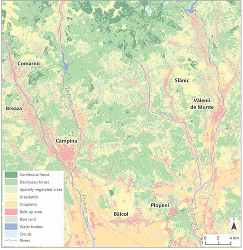
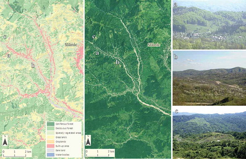
The land cover map for Subcarpathian area, obtained using SVM classification, algorithm has eight classes. The confusion issues were solved by using multi-date images (Figure 6a); therefore, the land cover categories are clearly presented on the map. The coniferous forest occupies small areas, situated in the northern part, close to the mountainous area. The settlement structure was well mapped, showing their spread and shape. Also, other built-up features are well represented, as the national road and the railway or industrial area from the south of study area. The sparsely vegetated class, which include orchards, shrubs and rare broadleaves trees, is located near the settlements and it is well represented on the map. The riverbeds of Prahova and Teleajen have a large extend at the contact of the Subcarpathians with the plain and in depressions (Figure 7).

Figure 6. Differences between single-date (1) and multi-date image classification (2) for Subcarpathian (1) and Carpathian (2) study areas.

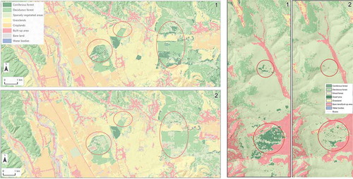
Figure 7. Land cover map for Subcarpathian area, generated from multi-date Sentinel-2 images, using SVM classification algorithm.

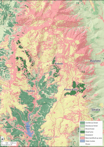
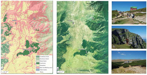
For Bucegi Massif, part of Bucegi Natural Park, the land cover map (Figure 8) obtained from Sentinel-2 images contains of 7 classes. The most complex category to differentiate was the mixed forest class (between fir, spruce and beech). Using two images for multi-date analysis (only from August 2015 and July 2016) helped for a better differentiation of this class (Figure 6b). Due to the same spectral reflectance, the built-up area had to be merged with the bare land surfaces in one category. This includes all the constructions, roads, tracks, as well as bare soil /rock or degraded grassland used for intensive grazing during the summer season. Compared with the orthophotos, the classification showed good results and a fine extraction of all tracks and details that could be seen on the plateau. The forest differentiation included coniferous (Picea abies, Abies alba, Larix decidua), beech (Fagus sylvatica), mixed forest and dwarf pine (Pinus mugo). Coniferous and dwarf pine covered areas were extracted very well, but some errors were encountered when differentiating beech and mixed forest. These are described in the confusion matrix in Table 6.

Table 4. Comparative table with statistical accuracies between ML and SVM for Subcarpathian and Carpathian area.

	Subcarpathian area					Carpathian area
		Producer’s accuracy		User’s accuracy			Producer’s accuracy		User’s accuracy
		ML	SVM	ML	SVM		ML	SVM	ML	SVM
Land cover classes	Coniferous	98.26	97.32	100.00	98.78	Coniferous	100.00	90.22	100.00	89.25
	Deciduous	98.54	97.55	95.33	98.43	Deciduous	98.46	100.00	100.00	98.48
	Sparsely vegetated area	21.24	45.05	93.96	57.88	Mixt forest	100.00	97.28	99.32	90.51
	Grasslands	98.27	97.1	83.03	85.46	Dwarf pine	96.25	68.75	100.00	82.09
	Cropland	91.86	76.43	98.05	97.75	Grassland	94.59	97.30	100.00	97.30
	Built-up area	99.74	96.52	57.46	94.08	Bare land/Built-up area	100.00	94.74	79.17	94.74
	Bare land	67.19	92.23	92.65	74.15	water bodies	100.00	100.00	100.00	100.00
	Water bodies	98.98	100.00	100.00	99.83
	Overall accuracy	ML 84.47%		SVM 92.41%		Overall accuracy	ML 98.65%		SVM 91.03%
	Kappa Coefficient	ML 0.8177		SVM 0.9098		Kappa Coefficient	ML 0.9829		SVM 0.8854

Table 5. Confusion matrix for Prahova–Teleajen Subcarpathians.

		Ground reference data									Total	User’s accuracy %	Commission error
	Classes	CF	G	BA	W	C	SV	C	BL	DF
CLASSIFIED IMAGE	Coniferous (CF)	97.32	0.00	0.00	0.00	0.00	0.00	0.00	0.00	0.30	6.47	98.78	1.22
	Grasslands (G)	0.00	97.10	0.00	0.00	2.28	54.95	0.00	0.00	0.00	16.22	85.46	14.54
	Built-up area (BA)	0.00	0.00	96.52	0.00	3.78	0.00	0.00	7.77	0.00	17.39	94.08	5.92
	Water bodies (W)	0.00	0.00	0.10	100.00	0.00	0.00	0.00	0.00	0.00	10.33	99.83	0.17
	Croplands (C)	0.00	0.92	0.62	0.00	76.43	0.00	0.00	0.00	0.00	10.57	97.75	2.25
	Sparsely vegetated areas (SV)	0.00	1.42	0.00	0.00	3.91	45.05	0.00	0.00	1.85	2.90	57.88	42.12
	Clouds (C)	0.00	0.00	0.00	0.00	0.00	0.00	100.00	0.00	0.30	1.42	94.41	5.59
	Bare land (BL)	0.00	0.55	2.75	0.00	11.85	0.00	0.00	92.23	0.00	8.31	74.15	25.85
	Deciduous (DF)	2.68	0.00	0.00	0.00	1.76	0.00	0.00	0.00	97.55	26.38	98.43	1.57
Producer’s accuracy %		97.32	97.10	96.52	100.00	76.43	45.05	100.00	92.23	97.55
Omission error		2.68	2.90	3.48	0.00	23.57	54.95	0.00	7.77	2.45
		Overall accuracy = 92.41					Kappa coefficient = 0.9098

Table 6. Confusion matrix for Bucegi Massif.

		Ground reference data							Total	User’s accuracy %	Commission error
	Classes	CF	DP	DF	MF	G	WB	B
CLASSIFIED IMAGE	Coniferous forest (CF)	100.0	0.00	0.00	0.00	0.00	0.00	0.00	20.63	100.0	0.00
	Dwarf pine (DP)	0.00	96.25	0.00	0.00	0.00	0.00	0.00	17.26	100.0	0.00
	Deciduous forest (DF)	0.00	0.00	98.46	0.00	0.00	0.00	0.00	14.35	100.0	0.00
	Mixed forest (MF)	0.00	0.00	1.54	100.0	0.00	0.00	0.00	33.18	99.32	0.68
	Grassland (G)	0.00	0.00	0.00	0.00	94.59	0.00	0.00	7.85	100.0	0.00
	Water bodies (WB)	0.00	0.00	0.00	0.00	0.00	100.0	0.00	1.35	100.0	0.00
	Bare land/built-up area (B)	0.00	3.75	0.00	0.00	5.41	0.00	100.0	5.38	79.17	20.83
Producer’s accuracy %		100.0	96.25	98.46	100.0	94.59	100.0	100.0
Omission error		0.00	3.75	1.54	0.00	5.41	0.00	0.00
		Overall accuracy = 98.65					Kappa coefficient = 0.9829

Figure 8. Land cover map for Bucegi area, generated from multi-date Sentinel-2 images, using ML classification algorithm.

Discussions

Using multi-date images in classification enhances the spectral separability of the land cover classes and increases the overall accuracy of the land cover map. The image pre-processing time increases, because the atmospheric and topographic corrections are applied on each data set.

The selection of training samples is also a difficult task, as they have to be statistically spectral different for generating a good accuracy of the classification. It is important to select samples from the field area or to validate them with expert knowledge.

The classification algorithms have to be chosen according to the land cover characteristics. We have chosen ML algorithm for the mountainous area where the land cover features were more compact and with clearly spectral behaviour. Otherwise, for Subcarpathian area, we used SVM, as the land cover classes were more fragmented and a lot of classes had similar spectral response. The resulted land cover maps have a high level of detail as they are produced from Sentinel-2 images at 10 m resolution (Table 4).

The overall accuracy of Subcarpathian land cover map of 92.41% (Table 5) shows a good correlation between the results of the classification and the reference data. The biggest omission affects sparsely vegetated class because of their spectral similarities with the grasslands on the fields covered with grasslands and shrubs. Other omission errors are affecting bare lands and croplands, where some pixels are committed in built-up area class. The user’s accuracy shows high values for water bodies, coniferous, deciduous and croplands. The lowest value of user’s accuracy refers to sparsely vegetated areas and bare lands.

For Bucegi Massif, the overall accuracy of the land cover map is 98.65% (Table 6). The highest scores for omission affects grassland and dwarf pine, mostly because of similar spectral response in some situations (degraded patches of grassland or isolated dwarf pines). Commission error, however, shows in some cases a significant difference between the classification and the reference data. For instance, the bare land/built-up area may have included some areas that were not necessarily in that category, because in many cases bare land areas are not clearly delimited along the Prahova abrupt, a very complex area. The second case represents the mixed forest areas, which may often include small compact patches of coniferous or deciduous forest that are generalized into one category, the resolution of the sensor being also a limitation.

We compared the results with orthophotos, but we also validated the land cover maps with field observations. In Figure 9, the images reflect the complexity of land cover features in the Subcarpathians. In Figure 9a, a settlement situated in the depression with pasture field nearby and deciduous forest (Fagus sylvatica) and also coniferous (Picea abies) on the interfluves is observed. In Figure 9b, the sparsely vegetated area class is well represented with fruit trees in blossom and other species of trees or shrubs situated on hill slopes, close to settlements. The Subcarpathian area is very fragmented by erosion and landslides that affect the slopes with soft rocks and no forested areas (Figure 9c).

Figure 9. SVM classification for Subcarpathian area, validated with orthophotos (2012) and field observations: (a) built-up area with pasture and forest, (b) sparse vegetation including fruit trees (plum and apple trees) and dispersed trees (acacia, hornbeam and willow), (c) sparse vegetation (shrubs) with pastures and bare lands.

A problem in the case of Bucegi Massif was to distinguish the built-up area from the bare land patches and that they had to be merged into one category. In Figure 10a, details from land cover map of Bucegi Massif are presented. Figure 10a illustrates Babele area with erosional areas due to touristic traffic and anthropogenic activities. This class, bare land and built-up area has the same spectral response and includes also areas like in Figure 10b with abrupt and rocky slopes (Caraiman abrupt). We mention the fact that for the Bucegi Natural Park management, the land cover map that includes the degraded areas represents a good solution for constant monitoring of the environmental evolution in the reservation. The third situation (Figure 10c) represents the Pinus mugo-covered area, protected inside the reservation, which was mostly mapped on the images except for the isolated patches/singular trees. Although highly fragmented, the plateau area from Bucegi Massif was well represented on the land cover map by each category with more details.

Figure 10. ML classification for Carpathian area, validated with orthophotos (2012) and field observations: (a) bare land with pasture and constructions, (b) rocky abrupt, (c) bare land with dwarf pine (Pinus mugo).

Conclusions

The input spectral bands, the training sets and classification algorithm represent key factors for land cover map production. The training samples created on multi-date images collect various spectral signatures of the land cover features in different seasons from the same year. Using multiple spectral bands from images acquired in different seasons, the accuracy of the final result enhances as the spectral separability between land cover features increase. The land cover maps generated from supervised classification of intra-annual multi-date images show higher levels of accuracies (92.41% for Subcarpathians and 98.65% for Carpathians) than the single-date classification. In the case of the hilly area with wide variety of land uses (discontinuous built-up areas, crops, orchards, together with sparsely wooden vegetation and deciduous and coniferous forests), a seasonal multi-date approach is necessary to separate the spectral signatures of the similar classes (for example, bare lands and croplands). In comparison, in the mountain area with compact and spectral-different features, the analysis is not necessary to include images from different seasons.

Choosing the processing algorithm depends on the characteristics of the land cover types. In this article, we have used two different algorithms for as our study regions were complementary: Prahova–Teleajen Subcarpathians with fragmented and heterogeneous features and Bucegi Massif with homogeneous vegetation layers.

The land cover maps that were obtained from Sentinel-2 calibrated images offer great level of detail with more than seven categories. They were validated in field, with ground truth data and orthophotos, being a good solution for spatial planning, hazard evaluation and protected areas management.

Using multi-date Sentinel-2 images involves time-consuming and important hardware resources, making it a difficult approach for casual uses. Also, in some situations, differentiating land cover categories with spectral similarities implies some issues due to spatial and spectral resolution.

Sentinel-2 MSI offers new possibilities for mapping land cover with greater precision that can be used for environmental monitoring, agriculture and forestry management, urban planning and decision making at local and regional scales.

Disclosure statement

No potential conflict of interest was reported by the authors.

References

- Anderson, J., Hardy, E.E., Roach, J.T., & Witmer, R.E. (1976). A land use and land cover classification system for use with remote sensing data.U.S. Geological Survey Professional Paper, No. 964 USGS, Washington DC.
- Arino, O., Bicheron, P., Achard, F., Latham, J., Witt, R., & Weber, J.-L. (2008). The most detailed portrait of Earth. Eur. Space Agency, 136, 25–31.
- Bartholomé, E., & Belward, A.S. (2005). GLC2000: A new approach to global land cover mapping from Earth observation data. International Journal of Remote Sensing, 26(9), 1959–1977. doi:10.1080/01431160412331291297
- Büttner, G., Feranec, J., & Jaffrain, G. (2000). Corine land cover update 2000. technical guidelines. Copenhagen, Denmark: European Environment Agency.
- Campbell, J.B., & Wynne, R.H. (2011). Introduction to remote sensing (5th ed.). New York; London: Guilford.
- Chen, J., Chen, J., Liao, A.P., Cao, X., Chen, L.J., Chen, X.H., ... Mills, l. (2015). Global land cover mapping at 30 m resolution: A POK-based operational approach. ISPRS Journal of Photogrammetry and Remote Sensing, 103, 7–27. doi:10.1016/j.isprsjprs.2014.09.002
- Chuvieco, E. Fundamentals of satellite remote sensing: An environmental approach. Second Edition. Boca Raton/London/New York: CRC Press Taylor & Francis. 2016
- Delegido, J., Verrelst, J., Alonso, L., & Moreno, J. (2011). Evaluation of Sentinel-2 Red-Edge Bands for empirical estimation of green LAI and chlorophyll content. Sensors, 11(7), 7063–7081. doi:10.3390/s110707063
- Di Gregorio, A., & Jansen, E. (1997). A new concept for a land cover classification system. Paper presented at the Earth Observation and Environmental Information 1997 Conference, Alexandria, Egipt.
- Di Gregorio, A., & Jansen, L.J.M. (2000). Land cover classification system (LCCS). Classification concepts and user manual for software version 1.0. Rome: FAO.
- Drusch, M., Del Bello, U., Carlier, S., Colin, O., Fernandez, V., Gascon, F., ... Bergellini, P. (2012). Sentinel-2: ESA’s optical high-resolution mission for GMES operational services. Remote Sensing of Environment, 120, 25–36. doi:10.1016/j.rse.2011.11.026
- ESA. (2015). Sentinel-2 user handbook. ESA Standard Document, 1(2). Retrieved January 2017 from https://sentinels.copernicus.eu/web/sentinel/user-guides/document-library/-/asset_publisher/xlslt4309D5h/content/sentinel-2-user-handbook
- Feranec, J., Hazeu, G., Christensen, S., & Jaffrain, G. (2007). Corine land cover change detection in Europe (case studies of the Netherlands and Slovakia). Land Use Policy, 24(1), 234–247. doi:10.1016/j.landusepol.2006.02.002
- Feranec, J., Hazeu, G., Jaffrain, G., & Cebecauer, T. (2007). Cartographic aspects of land cover change detection (over- and underestimation in the I&CORINE Land Cover 2000 Project). Cartographic Journal, 44(1), 44–54. doi:10.1179/000870407X173869
- Feranec, J., Jaffrain, G., Soukup, T., & Hazeu, G. (2010). Determining changes and flows in European landscapes 1990-2000 using CORINE land cover data. Applied Geography, 30(1), 19–35. doi:10.1016/j.apgeog.2009.07.003
- Gomez, C., White, J.C., & Wulder, M.A. (2016). Optical remotely sensed time series data for land cover classification: A review. Isprs Journal of Photogrammetry and Remote Sensing, 116, 55–72. doi:10.1016/j.isprsjprs.2016.03.008
- Hansen, M. (2012). Classification trees and mixed pixel trening data. In C. Giri (Ed.), Remote sensing of land use and land cover. priciples and applications (pp. 127–136). Boca Raton, London, New York: Taylor&Francis Group, CRC Press.
- Hansen, M.C., Defries, R.S., Townshend, J.R.G., & Sohlberg, R. (2000). Global land cover classification at 1 km spatial resolution using a classification tree approach. International Journal of Remote Sensing, 21(6–7), 1331–1364. doi:10.1080/014311600210209
- Hantson, S., & Chuvieco, E. (2011). Evaluation of different topographic correction methods for Landsat imagery. International Journal of Applied Earth Observation and Geoinformation, 13(5), 691–700. doi:10.1016/j.jag.2011.05.001
- ISO-19144-1. (2009). Geographic information — Classification systems — Part 1: Classification system structure (Vol. ISO 19144-1). Prepared by FAO, Published by the International Organisation for Standardization at https://www.iso.org/standard/32562.html
- ISO-19144-2. (2012). Geographic information - Classification systems – Part 2: Land Cover Meta Language (LCML) (pp. 107): ISO/TC 211 geographic information/geomatics.Prepared by FAO, Published by the International Organisation for Standardization at https://www.iso.org/standard/44342.html
- Khatami, R., Mountrakis, G., & Stehman, S.V. (2016). A meta-analysis of remote sensing research on supervised pixel-based land-cover image classification processes: General guidelines for practitioners and future research. Remote Sensing of Environment, 177, 89–100. doi:10.1016/j.rse.2016.02.028
- Latham, J., Cumani, R., Rosati, I., & Bloise, M. (2014). FAO global land cover (GLC-SHARE) beta-release 1.0 Database. Rome: FAO. Retrieved January 2017 from www.fao.org/uploads/media/glc-share-doc.pdf
- Lillesand, T.M.A., Kiefer, R.W.A., & Chipman, J.W.A. (2015). Remote sensing and image interpretation. 7th Edition, New York, NY: John Wiley & Sons
- Mayer, B., & Kylling, A. (2005). Technical note: The libRadtran software package for radiative transfer calculations - description and examples of use. Atmospheric Chemistry and Physics, 5, 1855–1877. doi:10.5194/acp-5-1855-2005
- Müller-Wilm, U. (2015). Sentinel-2 MSI - Level-2A prototype processor installation and user manual. Germany: Telespazio VEGA Deutschland GmbH.
- Parmentier, B., & Eastman, J.R. (2014). Land transitions from multivariate time series: Using seasonal trend analysis and segmentation to detect land-cover changes. International Journal of Remote Sensing, 35(2), 671–692. doi:10.1080/01431161.2013.871595
- Riano, D., Chuvieco, E., Salas, J., & Aguado, I. (2003). Assessment of different topographic corrections in Landsat-TM data for mapping vegetation types. Transactions on Geoscience and Remote Sensing, 41(5), 1056–1061. doi:10.1109/TGRS.2003.811693
- Robin, M. (1998). La Télédetection. Paris: Editions Nathan.
- Rujoiu-Mare, M.R., & Mihai, B. (2016). Mapping land cover using remote sensing data and GIS techniques: A case study of Prahova Subcarpathians. Elsevier Procedia Environmental Sciences, 32, 244–255. doi:10.1016/j.proenv.2016.03.029
- Sârbu, A., Anastasiu, P., Smarandache, D., Pascale, G., Lițescu, S., & Mihai, D.C. (2013). Habitate cu valoare conservativă din Parcul Natural Bucegi. Bucharest: Ceres Publisher House.
- Schowengerdt, R.A. (ed.). (2007). Remote sensing: Models and methods for image processing (3rd ed.). London: Academic Press.
- Sexton, J.O., Urban, D.L., Donohue, M.J., & Song, C.H. (2013). Long-term land cover dynamics by multi-temporal classification across the Landsat-5 record. Remote Sensing of Environment, 128, 246–258. doi:10.1016/j.rse.2012.10.010
- Shao, Y., Lunetta, R.S., Wheeler, B., Iiames, J.S., & Campbell, J.B. (2016). An evaluation of time-series smoothing algorithms for land-cover classifications using MODIS-NDVI multi-temporal data. Remote Sensing of Environment, 174, 258–265. doi:10.1016/j.rse.2015.12.023
- Teillet, P.M., Guindon, B., & Goodenough, D.G. (1982). On the slope-aspect correction of multispectral scanner data. Canadian Journal of Remote Sensing(8), 84–106. doi:10.1080/07038992.1982.10855028
- USGS. (2016). Landsat 8 (L8) data users handbook Version 2.0. Department of the Interior U.S. Geological Survey. Retrieved December 2016 from https://landsat.usgs.gov/…/Landsat8DataUsersHandbook.pdf
- Vanonckelen, S., Lhermitte, S., & Van Rompaey, A. (2013). The effect of atmospheric and topographic correction methods on land cover classification accuracy. International Journal of Applied Earth Observation and Geoinformation, 24, 9–21. doi:10.1016/j.jag.2013.02.003
- Wulder, M.A., Hilker, T., White, J.C., Coops, N.C., Masek, J.G., Pflugmacher, D., Crevier, Y. (2015). Virtual constellations for global terrestrial monitoring. Remote Sensing of Environment, 170, 62–76. doi:10.1016/j.rse.2015.09.001