
ABSTRACT
In the presented study, the Sentinel-2 vegetation indices (VIs) were evaluated in context of estimating defoliation of Scots pine stands in western Poland. Regression and classification models were built based on reference data from 50 field plots and Sentinel-2 satellite images from three acquisition dates. Three machine-learning (ML) methods were tested: k-nearest neighbors (kNN), random forest (RF), and support vector machines (SVM). Regression models predicted stands defoliation with moderate accuracy. R2 values for regression models amounted to 0.53, 0.57, 0.57 for kNN, RF and SVM, accordingly. Analogically, the following values of normalized root mean squared error were obtained: 12.2%, 11.9% and 11.6%. Overall accuracies for two-class classification models were 78%, 75%, 78% for kNN, RF and SVM methods. The Green Normalized Difference Vegetation Index and MERIS Terrestrial Chlorophyll Index VIs were found to be most robust defoliation predictors regardless of the ML method. We conclude that Sentinel-2 satellite images provide useful information about forest defoliation and may contribute to forest monitoring systems.
Introduction
Remote sensing (RS) is as a technology that contributes to forest health assessment and monitoring (Pause et al., Citation2016; Wulder & Franklin, Citation2003). Assessment of forest health indicators and understanding the influence of different stress factors often require a combination of in-situ terrestrial observations and remote-sensing data (Trumbore, Brando, & Hartmann, Citation2015). In-situ terrestrial data are usually collected on a plot level, while RS data provide wall-to-wall information on multiple temporal and spatial scales (Lausch, Erasmi, King, Magdon, & Heurich, Citation2017). Examples of forest health indicators include visible assessment of infestation levels, leaf defoliation and discoloration, amount of dead branches, trunk damage, number or volume of standing, dead and fallen trees, crown closure or the leaf area index (Lausch, Erasmi, King, Magdon, & Heurich, Citation2016).
One of an important indicator used for assessment of forest health is defoliation (Innes, Citation1993). The monitoring concept of trees health survey based on defoliation lays in relationship between tree crowns condition which reflects the tree health. For practical applications, defoliation values are often grouped into classes: <=10% – none, >10–25 – slight, >25–60% – moderate, >60–<100% – severe and 100% – dead. Exceed of the 25% defoliation threshold is considered as an early warning signal of tree weakness (UNECE ICP Forests Programme; Michel & Seidling, Citation2016). The deterioration of tree crown may be induced by many factors like chemical pollution, drought, fungus pathogens, insects etc.; thus, the defoliation assessment is usually challenging issue.
Many studies evaluating the applicability of RS for assessment of forest defoliation were conducted (Eigirdas, Augustaitis, & Mozgeris, Citation2013; Ekstrand, Citation1994; Hall, Castilla, White, Cooke, & Skakun, Citation2016; Mozgeris & Augustaitis, Citation2013; Rullan-Silva, Olthoff, Delgado de la Mata, & Pajares-Alonso, Citation2013). Aerial images are one of the most widely used RS data for forest health assessments with long history (Hall, Citation2003); however in context of forest defoliation, other RS data sources like airborne laser scanning (Kantola et al., Citation2010; Solberg, Citation2010; Solberg, Næsset, Hanssen, & Christiansen, Citation2006) and satellite images (Adelabu, Mutanga, & Adam, Citation2014; Eklundh, Johansson, & Solberg, Citation2009; Townsend et al., Citation2012) are used as well. A variety of different methods are utilized for defoliation assessment based on RS data including spectral mixture analysis (Somers et al., Citation2010), time series analysis (Spruce et al., Citation2011) and vegetation indices (VIs) analysis (de Beurs & Townsend, Citation2008; Townsend et al., Citation2012).
One of the most widely used VI in context of forest defoliation is the normalized difference vegetation index (NDVI; Rullan-Silva et al., Citation2013). In many studies, it was found to be robust VI for defoliation mapping (Jepsen et al., Citation2009; Kharuk, Ranson, & Im, Citation2009; Marx & Kleinschmit, Citation2017; Spruce et al., Citation2011). However, some studies showed that other VIs may surpass the NDVI. There are known examples were short wave infrared (SWIR)-based VIs were more suitable for defoliation monitoring than the NDVI (de Beurs & Townsend, Citation2008; Sangüesa-Barreda, Camarero, García-Martín, Hernández, & De la Riva, Citation2014; Townsend et al., Citation2012). The red-edge-based VIs were also found to be robust in defoliation assessment (Adelabu et al., Citation2014; Coops et al., Citation2003). It was stated by Rullan-Silva et al. (Citation2013) that performance of VIs in context of forest defoliation may vary from site to site; thus, it is recommended to explore different VIs in each particular case.
In 2015, the European Space Agency (ESA) lunched the Sentinel-2A satellite and in 2017, the Sentinel-2 constellation was extended with Sentiel-2B satellite. The Sentinel-2 tandem has several advantages comparing to existing Earth Observation systems used for forest defoliation assessment up to now (Drusch et al., Citation2012). The data have comparable spatial resolution to commercial SPOT or RapidEye systems but are free of charge. Comparing to the Landsat mission the Sentinel-2 provides the red-edge spectral bands what extends its potential usefulness for analysis of vegetation. Sentinel-2 data clearly surpass the MODIS data in context of spatial resolution (10–20 vs. 250 m). For these reasons, it seems to be justified to investigate the potential suitability of Sentinal-2 data for forest defoliation assessment.
The usefulness of VIs derived from Sentinel-2 data for estimation of Scots pine stands defoliation has not been investigated before to our knowledge. There is also limited number of studies where machine-learning (ML) methods were used in context of forest defoliation analysis (Adelabu et al., Citation2014; Kantola et al., Citation2010; Marx & Kleinschmit, Citation2017). Based on the experience of other researchers who investigated variety of satellite sensors for forest defoliation assessment, we see Sentinel-2 images as a valuable source of data for such applications. In this context, the two main goals of the study were defined (1) to identify the most robust Sentinel-2-derived VIs for Scots pine stands defoliation assessment at plot level regardless of applied ML method and (2) to compare the performance of regression and classification models created based on different ML approaches.
Materials and methods
Study area
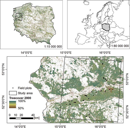
The study area of approximately 10,000 km2 was located in the western Poland including the Puszcza Notecka Forest, one of the largest contiguous forest complexes in Poland (). The forest stands in this region are dominated by Scots pine (Pinus sylvestris L.) which covers 88% of the study area. The study site was selected based on annual reports about condition of forests prepared by The Polish State Forests (Milewski, Citation2015). The idea was to select a site were defoliation of Scots pine stands can be observed. According to the report in the selected region, there was observed an increased occurrence of Pine-tree lappet (Dendrolimus pini L.) which is one of the main insect defoliator of Scots pine forests in Poland during last years.
Figure 1. Location of the study area. “Treecover 2000” was obtained from Global Forest Change (Hansen et al., Citation2013).
Field data
To capture the stands defoliation variability in the satellite data, the Enhanced Vegetation Index (EVI) calculated from Landsat 8 satellite images was used in the first step. The difference of EVI values between 2 August 2015 and 18 March 2015 was calculated for the whole study area. It was assumed that the calculated difference is connected with defoliation of stands. The obtained difference raster layer was then reclassified into 25 strata. For each strata with minimum area of nine pixels (3 × 3 pixels), two field plots were randomly placed.
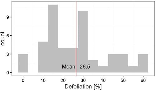
The field campaign was performed on 50 filed plots in September 2015. The plots were placed in single-species Scots pine stands with only single trees of Silver birch (Betula pendula Roth) and age from 21 to 60, growing on relatively poor sandy soils within the same forest site type. Selection of these stands was based on the existing Digital Forest Map and we assumed that the stands should have comparable stand reflectance; thus, the stand defoliation can be observed on satellite images. Plot locations were derived using GNSS receiver (Spectra Precision MobileMapper 120) equipped with an external antenna to achieve submeter precision. Defoliation of a tree was assessed visually in 5% classes. To assess the tree defoliation level, the tree defoliation scale proposed by Polish Forest Research Institute and photo guides of assimilative apparatus loss were used (Borecki & Keczyński, Citation1992; Müller & Stierlin, Citation1990). The guide of reference trees takes into account the age of tree. Defoliation was defined as needle loss in the assessable crown comparing to a photo of the reference tree. The defoliation value for a plot was calculated as the mean defoliation value of the 20 trees from the dominant stand (Kraft’s classification) closest to the plot center. Only trees from the first three Kraft’s classes were considered (predominant, dominant and codominant) since it was assumed that they mostly influence the plot reflectance. The approximate radius of field plots varied from about 5 to 20 m depending on the age of the trees. Histogram of defoliation values obtained at plot level is presented in .
Figure 2. Histogram of defoliation values obtained in field plots level (n = 50).
RS data processing
Regression and classification models of defoliation were built using VIs of three Sentinel-2 satellite images. Sentinel-2 provides images with 13 spectral bands spanned from the visible (VIS) and the near infrared to the SWIR. The bands have different ground sampling distances (Drusch et al., Citation2012). The four bands are at 10 m spatial resolution (B2 – 490 nm, B3 – 560 nm, B4 – 665 nm, B8 – 842 nm), the six bands at 20 m resolution (B5 – 705 nm, B6 – 740 nm, B7 – 783 nm, B8a – 865 nm, B11 – 1610 nm, B12 – 2190 nm) and the three bands at 60 m resolution (B1 – 443 nm, B9 – 940 nm, B10 – 1375 nm).
The idea was to use all available cloud-free Sentinel-2 images for the study area. Finally, only three images were appropriate. The following acquisition dates were used: 4 July 2015, 20 August 2015 and 17 March 2016. The data were obtained from the Copernicus Open Access Hub (https://scihub.copernicus.eu/dhus/#/home) as Level-1C data with top of atmosphere reflectance. The Level-1C images were processed to Level-2A bottom-of-atmosphere (BOA) product using ESA SNAP Sentinel 2 Toolbox with additional Sen2Cor plug-in for atmospheric correction. The atmospheric correction in this software package is based on the application of look-up-tables, which were pre-calculated using the libRadtran – a collection of C and Fortran functions and programs for calculation of solar and thermal radiation in the Earth (Emde et al., Citation2016; Vuolo et al., Citation2016). The BOA surface reflectance images were generated in 20 m spatial resolution. Then for each plot center, the VIs reported in were calculated for each acquisition date and subsequently used as predictor variables in regression and classification models.
Table 1. Vegetation indices used as predictor variables for building regression and classification models of defoliation.
Building regression and classification models
The three ML methods were used for creating regression and classification models: k-nearest neighbors (kNN), random forest (RF) and support vector machines (SVM) as they are one of the most widely used ML methods in the field of RS (López-Serrano, López-Sánchez, Álvarez-González, & García-Gutiérrez, Citation2016).
The kNN method predicts a new sample using the k-nearest samples from the training set. In case of regression, a predicted response of new sample is usually the mean of the k-neighbors responses. For classification, a class probability estimates for the new sample are calculated as the proportion of training set neighbors in each class. The class with the highest estimated probability is treated as result of prediction. The optimal number of neighbors used for prediction can be estimated by one of the resampling method like k-fold cross-validation, leave-one-out cross-validation or bootstrap (Altman, Citation1992; Cover & Hart, Citation1967; Kuhn & Johnson, Citation2013). In the presented study, the Euclidean distance metric which was used to measure the distance between samples and the final estimate for regression was calculated as the mean of the neighbors. The optimal number of neighbors was searched from sequence of integers from 1 to 20.
The SVM was originally developed in the context of classification models (Cortes & Vapnik, Citation1995) and was later extended for regression (Drucker, Burges, Kaufman, Smola, & Vapnik, Citation1997; Smola & Schölkopf, Citation2004). In principle, the SVM classification algorithm aims to find a hyperplane that separates the dataset into a discrete predefined number of classes using training examples. The optimal separation hyperplane is used to minimize misclassifications, obtained in the training step (Mountrakis, Im, & Ogole, Citation2011). General idea of SVM in context of regression modeling is that the observations with residuals lying within user-defined threshold do not contribute to the regression fit while observations with residuals greater than the threshold contribute in a linear-scale amount. Consequently, since the squared residuals are not used, large outliers have a limited effect on the regression equation and simultaneously samples with small residuals have no effect on the regression equation (Kuhn & Johnson, Citation2013). In the reported study, the SVM with polynomial kernel was applied and the following values of tuning parameters were tested: polynomial degree: 1, 2; scale: 0.01, 0.005, 0.001; cost: 0.25, 0.5, 1, 2. 4, 8, 16, 32, 64, 128.
RF is ensemble of a defined number (n) of simple decision trees, which are used to determine the final outcome. Each tree is independently determined using a bootstrap sample of the data. Each model in the ensemble is used to generate a prediction for a new sample and these predictions are averaged to obtain the forest’s prediction. For classification problems, the trees vote for the most popular class. In the regression problem, trees’ responses are averaged to obtain an estimate of the dependent variable. The RF algorithm randomly selects defined number of predictors (mtry) at each split to reduce correlation among trees (Breiman, Citation2001; Hultquist, Chen, & Zhao, Citation2014). The number of trees for the forest in the study was set to 1000 for both regression and classification models. The mtry parameter was tuned from the following values: 2, 5, 9, 13, 17, 21, 25, 29, 33, 37 to find the best model.
Predictive models were built using the R caret package (Kuhn, Citation2008). For kNN, RF and SVM additional R packages: class (Venables & Ripley, Citation2002), randomForest (Liaw & Wiener, Citation2002) and kernlab (Karatzoglou, Smola, Hornik, & Zeileis, Citation2004) were used, accordingly. The same tuning parameters were tested for classification and regression models within ML methods excepting kNN where in case of two-class classification problems, it is recommended to use odd values of neighbors. As response variable in regression, the percentage value of defoliation was used. For classification, two classes were distinguished: slight defoliation (defoliation ≤ 25%) and moderate defoliation (25% < defoliation ≤ 60%). Classes were created referring to Hanisch and Kilz (Citation1990); however, because of relatively small number of field observations (50), the class of none defoliation (≤10%) distinguished by these authors was merged with class slight defoliation. It resulted in 27 observations for slight and 23 observations for moderate defoliation.
The first step of analysis was removing highly correlated predictor variables. Correlation matrix for VIS was created for the first acquisition date (4 July 2015) using Pearson correlation coefficient. For a pair of predictor variables with the correlation coefficient higher than 0.9, the variable with lower correlation to the response variable was dropped. Correlation matrix was then created again to remove correlated values of VIs between acquisition dates. Variables with near zero variance were removed in the next step. Then, the feature selection process was performed for regression models separately for each ML method. In case of kNN and SVM, all predictors were preprocessed by centering and scaling. The selected best variables for each method were subsequently used for classification as well. A backward selection algorithm called recursive feature elimination (RFE) described by Guyon, Weston, Barnhill and Vapnik (Citation2002) was used for selection of best predictors. In the first step of RFE, the full model is created and a measure of variable importance is computed that ranks the predictors from most important to least. At each stage of the search, the features with lowest importance are iteratively pruned prior to rebuilding the model. Once a new model is created, the objective function is estimated for that model based on cross-validation. Optimization of model’s tuning parameters can be performed using additional inner resampling loop. That procedure is recursively repeated for some predefined sequence, and the subset size corresponding to the best value of the objective function is used as the final model (Kuhn & Johnson, Citation2013). The algorithm was configured to explore the sequence of subsets of variables from 2 to 38 increasing by 2. Finally, the variable’s importance values were computed using the ranking method applied in feature selection. For the selected optimal subset of predictor variables within each tested ML method, the variable’s importance values from the models across all resamples were averaged to compute an overall importance. For easier comparison between tested ML methods, the relative variable’s importance values were calculated by scaling the obtained importance measures to have a maximum value of 100.
Performance of models was assessed using a 10-fold cross-validation repeated five times. Thus, 50 different hold-out datasets were used to assess the final model’s performance. As performance metrics for regression, the normalized root mean squared error (nRMSE) and R-squared (R2) were used. The nRMSE was calculated as the RMSE averaged from 50 hold-out sets divided by the mean defoliation value of all sample plots and multiplied by 100%. For classification models, the overall accuracy and kappa coefficient were calculated. Based on confusion matrices, also commission and omission errors were calculated for classification models.
Results selected VIs
The 23 VIs obtained from 3 Sentinel-2 images were calculated what gave 69 predictor variables in total. After removing of highly correlated and near zero variance variables, the final set of 38 variables was used as input for RFE (). As result of feature selection process, 10, 14 and 26 number of variables were selected as optimal subset sizes for kNN, RF and SVM methods, respectively.
Figure 3. Relative importance values calculated for VIs in regression models of tested ML methods (SVM: support vector machines; RF: random forest; kNN: k-nearest neighbors).
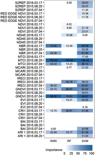
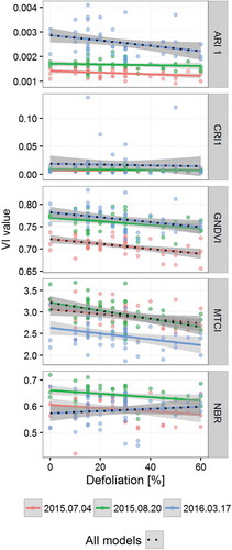
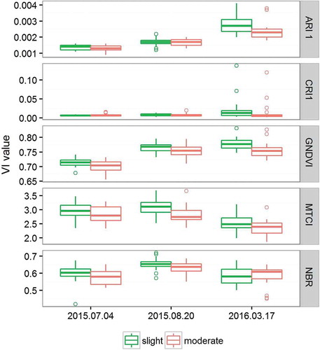
Relative importance of variables was calculated for each method (). Two predictor variables – MERIS Terrestrial Chlorophyll Index (MTCI) 20 August 2015 and Green Normalized Difference Vegetation Index (GNDVI) 4 July 2015 – achieved high importance in all tested ML methods. The following predictor variables were selected through RFE for all ML methods: ARI 1, CRI 1, GNDVI, MTCI and NBR. The relationship between values of these VIs and defoliation are presented on . What should be noted is that for all acquisition dates, GNDVI and MTCI values decreased with increasing defoliation. The same relationship is observed for ARI 1 17 March 2016. Values of NBR from three acquisition dates showed different relationship with defoliation values.
Figure 4. Relationship between selected VIs and defoliation values.
Analysis of distribution of VIs values showed that their trends through acquisition dates were different (). MTCI values decrease from first to third acquisition date in both defoliation classes while GNDVI showed increasing trend. For both Vis, their values were lower for class moderate than for slight defoliation. High increase for ARI 1 17 March 2016 is observed for both classes comparing to the previous acquisition dates. Differences between defilation classes in values of ARI 1 and CRI 1 appeared in 17 March 2016 when class moderate had lower values for these VIs. Differences in ARI 1 and CRI 1 between classes were not observed in previous dates.
Figure 5. Distribution of selected VIs’ values in two defoliation classes and three acquisition dates (slight: slight defoliation, moderate: moderate defoliation).
Performance of regression and classification models
For each ML method, the optimal values of tuning parameters were found through cross-validation. The optimal values of tuning parameters for kNN and RF were found the same for classification and regression models: 5 as the number of neighbors in kNN and 2 as number of randomly selected predictors in RF. In case of SVM, the following values of tuning parameters were found to be optimal: polynomial degree = 1, scale = 0.001 and cost = 64 (regression); polynomial degree = 2, scale = 0.001 and cost = 4 (classification).
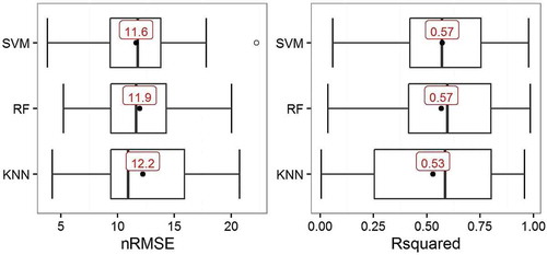
All regression models predicted stand defoliation with moderate accuracy. The nRMSE value was the lowest for SVM – 11.6% with 11.9% for RF and 12.2% for kNN. R2 varied from 0.53 (kNN) to 0.57 (RF and SVM). The distributions of nRMSE values for RF and SVM obtained through cross-validation were very similar (). Validation results indicated that kNN model was less stable than RF and SVM through cross-validation.
Figure 6. nRMSE and R2 values for regression models obtained through cross-validation (SVM: support vector machines; RF: random forest; kNN: k-nearest neighbors).
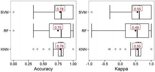
The achieved accuracies of classification models were moderate as well. The RF model achieved the lowest overall accuracy of 0.75 and corresponding kappa coefficient of 0.49. kNN and SVM models achieved the same overall accuracy and kappa of 0.78 and 0.55, respectively. Analysis of distribution of performance metrics obtained from cross-validation showed that SVM model was more stable although kNN provided the same mean values of accuracy and kappa ().
Figure 7. Overall accuracy and kappa coefficient values for classification models obtained through cross-validation (SVM: support vector machines; RF: random forest; kNN: k-nearest neighbors).
Confusion matrices obtained from cross-validation were very similar for kNN and SVM methods (). In these methods, the tendency to underestimation of class moderate was observed with omission errors of 0.33 and 0.32, respectively. The commission and omission errors were similar for both classes in case of RF method. The commission errors for class slight defoliation were equal for all methods and amounted to 0.24. The lowest error of omission for class slight defoliation was achieved in kNN method (0.13).
Table 2. Confusion matrices of classification models obtained through cross-validation (SVM: support vector machines; RF: random forest; kNN: k-nearest neighbors).
Discussion
In the presented study, we investigated the usability of selected VIs derived from Sentinel-2 satellite data in context of Scots pine stands defoliation assessment at plot level using three ML methods: kNN, RF and SVM.
Although the NDVI is the most widely used VI in context of forest defoliation assessment (Rullan-Silva et al., Citation2013), it was not found to be robust in our study. Instead, we found GNDVI to be more suitable. Assuming that with increasing defoliation, the total amount of chlorophyll in the canopy decreases, our results are in line with Gitelson, Kaufman and Merzlyak (Citation1996) who found GNDVI correlated with chlorophyll concentration at leaf level. The GNDVI was also found to be more sensitive than NDVI for burn severity assessment at canopy level (Fernández-Manso, Fernández-Manso, & Quintano, Citation2016). The GNDVI was also found to be correlated with leaf area index (Szporak-Wasilewska et al., Citation2014); thus, the higher value of GNDVI in 20 August 2015 and 17 March 2016 comparing to 4 July 2015 suggests that the observed defoliation occurred before 4 July 2015. The reason that NDVI was not found to be robust predictor in our study may be the fact that we do not observed plots with very severe defoliation. As suggested by Marx and Kleinschmit (Citation2017), the correlation between NDVI and defoliation is higher for more severe defoliation classes.
The MTCI value from 20 August 2015 was found to be the most robust predictor variable in our study (). The MTCI was found by Dash and Curran (Citation2007) to be a suitable VI for the estimation of chlorophyll content with MERIS data. In the MTCI formula, the red (B4) and two red-edge bands (B5 and B6) are used (). The importance of MTCI indicates that the red-edge spectral range is sensitive for defoliation of Scots pine stands. Similar findings are known from previous studies (Adelabu et al., Citation2014; Coops et al., Citation2003; Marx & Kleinschmit, Citation2017). Negative correlation of GNDVI and MTCI with defoliation values () suggesting decrease of chlorophyll content in needles is in line with the results obtained by Roitto et al. (Citation2003). Decrease of MTCI values in 17 March 2016 comparing to 20 August 2015 and 4 July 2015 images may have an effect of lover chlorophyll content in the needles and less photosynthetic activity in March than in summer months.
Decrease of MTCI in 17 March 2016 was accompanied by increase of CRI 1 and ARI 1 values. Higher values of CRI 1 for slight defoliation class than for moderate defoliation in 17 March 2016 image are in opposite to findings of Roitto et al. (Citation2003) who observed a slight increase of carotenoids concentration in needles of defoliated Scots pine trees. It should be stressed, however, that CRI 1 was developed for leaves of deciduous species (Gitelson, Zur, Chivkunova, & Merzlyak, Citation2002). The increase of ARI 1 was higher than CRI 1 what indicates higher increase of anthocyanin concentration comparing to carotenoids (Gitelson et al., Citation2001, Citation2002). Among many functions that anthocyanins play in plant physiology, they are induced as a response to ultraviolet (UV-B) radiation (Chalker-Scott, Citation1999; Stapleton, Citation1992). Since ARI 1 was developed for different plant species, it is not clear whether it describes exclusively anthocyanins in case of Scots pine. All the more so the synthesis of anthocyanins depend on the host species, pH, aggregation of other pigments, flavonols and metal complexing (Gitelson et al., Citation2001).
In the presented study, also the NBR (NDII12) index showed to be useful for defoliation assessment; however, its values varied significantly between acquisition dates. The NBR values were expected to be negatively correlated with defoliation; however, it was the case only for 4 July 2015 and 20 August 2015 images while for the 17 March 2016 image, the correlation was slightly positive (). Since NDII11 and NDII12 were highly correlated (Pearson correlation >0.97), only the NDII12 (NBR) was used for creating regression and classification models. Analogical indices to NDII11 and NDII12 (NBR), but calculated from Landsat ETM+ data, were used by Townsend et al. (Citation2012) who found them robust for assessment of canopy defoliation in broadleaf deciduous forests.
Some limitations of the presented study should be considered. The investigated stands were single-species Scots pine forests growing on relatively poor sandy soils within the same site type; thus, the influence of the ground vegetation on the spectral response of the forest canopy was limited. Different results may be achieved for stands on different site types and with lush understory. Sentinel-2 images acquired only after the highest potential defoliation occurrence were available for this study. The accuracy of regression and classification models may increase in case of using also the images acquired in early spring of 2015. The available pre-defoliation data from Landsat 8 satellite were not used intentionally in regression and classification models since the idea was to investigate only the Sentinel-2 data. However, the Landsat 8 images were used for stands stratification and random selection of field plots.
Conclusions
VIs calculated based on Sentinel-2 satellite images and used with ML methods enable assessment of Scots pine stands defoliation with moderate accuracy using regression and classification models. kNN, RF and SVM methods predict defoliation with similar accuracy with preference to SVM as assessed by cross-validation to be the most stable method. Different ML methods use different VIs as optimal predictor variables for the same dataset however selected VIs such as MTCI and GNDVI are robust regardless of the ML approach. In case of images acquired at the beginning of vegetation season, also the VIs describing the carotenoids (CRI 1) and anthocyanins (ARI 1) concentration provide useful information for defoliation assessment. The SWIR-based index – NBR (NDII12) – is also suitable in context of Scots pine defoliation assessment. Using single VI does not guarantee achievement of high accuracy; thus, it can be recommended to use many VIs as predictor variables in ML-based regression and classification models of Scots pine defoliation. Further research is needed to investigate the possibility of Sentinel-2 data for defoliation assessment especially in context of using images acquired before and after defoliation occurrence what may increase the accuracy of predictive models. Sentinel-2 system is a promising source of data that can contribute to development of forest defoliation assessment methods.
Geolocation information
50°04ʹ58.5ʺN, 19°57ʹ04.0ʺE.
Disclosure statement
No potential conflict of interest was reported by the authors.
Additional information
Funding
References
- Adelabu, S., Mutanga, O., & Adam, E. (2014). Evaluating the impact of red-edge band from Rapideye image for classifying insect defoliation levels. ISPRS Journal of Photogrammetry and Remote Sensing, 95, 34–41.
- Altman, N.S. (1992). An introduction to kernel and nearest-neighbor nonparametric regression. The American Statistician, 46(3), 175–185.
- Borecki, T., & Keczyński, A. (1992). Atlas ubytku aparatu asymilacyjnego drzew leśnych [Photo guide of assimilative apparatus loss of trees]. Warszawa: Agencja Reklamowa “ATUT”.
- Breiman, L. (2001). Random forests. Machine Learning, 45(1), 5–32.
- Blackburn, G. A. (1998). Spectral indices for estimating photosynthetic pigment concentrations: A test using senescent tree leaves. International Journal of Remote Sensing, 19(4),657–675. https://doi.org/10.1080/014311698215919
- Clevers, J. G. P. W., Jong, S. M. De, Epema, G. F., Addink, E. a, & Box, P. O. (2000). Meris and the Red-Edge Index. In 2nd EARSeL workshop, Enschede, 2000 (pp. 1–16).
- Chalker-Scott, L. (1999). Environmental significance of anthocyanins in plant stress responses. Photochemistry and Photobiology, 70(1), 1–9.
- Chuvieco, E., Martín, M. P., & Palacios, A. (2002). Assessment of different spectral indices in the red-near-infrared spectral domain for burned land discrimination. International Journal of Remote Sensing, 23 (23), 5103–5110. https://doi.org/10.1080/01431160210153129
- Coops, N., Stanford, M., Old, K.M., Dudzinski, M.J., Culvenor, D., & Stone, C. (2003). Assessment of dothistroma needle blight of pinus radiata using airborne hyperspectral imagery. Phytopathology, 93(12), 1524–1532.
- Cortes, C., & Vapnik, V. (1995). Support vector networks. Machine Learning, 20(3), 273–297.
- Cover, T., & Hart, P. (1967). Nearest neighbor pattern classification. IEEE Transactions on Information Theory, 13, 21–27.
- Dash, J., & Curran, P.J. (2007). Evaluation of the MERIS terrestrial chlorophyll index (MTCI). Advances in Space Research, 39(1), 100–104.
- de Beurs, K.M., & Townsend, P.A. (2008). Estimating the effect of gypsy moth defoliation using MODIS. Remote Sensing of Environment, 112(10), 3983–3990.
- Drucker, H., Burges, C.J.C., Kaufman, L., Smola, A., & Vapnik, V. (1997). Support vector regression machines. Advances in Neural Information Processing Dystems, 1, 155–161.
- Daughtry, C. (2000). Estimating Corn Leaf Chlorophyll Concentration from Leaf and Canopy Reflectance. Remote Sensing of Environment, 74(2),229–239. https://doi.org/10.1016/S0034-4257(00)00113-9
- Drusch, M., Del Bello, U., Carlier, S., Colin, O., Fernandez, V., Gascon, F., … Bargellini, P. (2012). Sentinel-2: ESA’s optical high-resolution mission for GMES operational services. Remote Sensing of Environment, 120, 25–36.
- Eigirdas, M., Augustaitis, A., & Mozgeris, G. (2013). Predicting tree crown defoliation using color-infrared orthophoto maps. IForest, 6(1), 23–29.
- Eklundh, L., Johansson, T., & Solberg, S. (2009). Mapping insect defoliation in Scots pine with MODIS time-series data. Remote Sensing of Environment, 113(7), 1566–1573.
- Ekstrand, S. (1994). Close range forest defoliation effects of traffic emissions assessed using aerial photography. Science of the Total Environment, 146-147, 149–155.
- Emde, C., Buras-Schnell, R., Kylling, A., Mayer, B., Gasteiger, J., Hamann, U., … Bugliaro, L. (2016). The libRadtran software package for radiative transfer calculations (version 2.0.1). Geoscientific Model Development, 9(5), 1647–1672.
- Fernández-Manso, A., Fernández-Manso, O., & Quintano, C. (2016). SENTINEL-2A red-edge spectral indices suitability for discriminating burn severity. International Journal of Applied Earth Observation and Geoinformation, 50, 170–175.
- Frampton, W. J., Dash, J., Watmough, G., & Milton, E. J. (2013). Evaluating the capabilities of Sentinel-2 for quantitative estimation of biophysical variables in vegetation. ISPRS Journal of Photogrammetry and Remote Sensing, 82, 83–92. https://doi.org/10.1016/j.isprsjprs.2013.04.007
- Gao, B. C. (1996). NDWI - A normalized difference water index for remote sensing of vegetation liquid water from space. Remote Sensing of Environment, 58(3),257–266. https://doi.org/10.1016/S0034-4257(96)00067-3
- Gitelson, A.A., Kaufman, Y.J., & Merzlyak, M.N. (1996). Use of a green channel in remote sensing of global vegetation from EOS-MODIS. Remote Sensing of Environment, 58(3), 289–298.
- Gitelson, A.A., Merzlyak, M.N., Chivkunova, O.B., Gitelson, A.A., Merzlyak, M.N., & Chivkunova, O.B. (2001). Optical properties and nondestructive estimation of anthocyanin content in plant leaves. Photochemistry and Photobiology, 74(1), 38–45.
- Gitelson, A.A., Zur, Y., Chivkunova, O.B., & Merzlyak, M.N. (2002). Assessing carotenoid content in plant leaves with reflectance spectroscopy. Photochemistry and Photobiology, 75(3), 272–281.
- Gitelson, A. A., Viña, A., Arkebauer, T. J., Rundquist, D. C., Keydan, G., & Leavitt, B. (2003). Remote estimation of leaf area index and green leaf biomass in maize canopies. Geophysical Research Letters, 30(5), n/a-n/a. https://doi.org/10.1029/2002GL016450
- Gitelson, A. A., Viña, A., Arkebauer, T. J., Rundquist, D. C., Keydan, G., & Leavitt, B. (2003). Remote estimation of leaf area index and green leaf biomass in maize canopies. Geophysical Research Letters, 30(5), n/a-n/a. https://doi.org/10.1029/2002GL016450
- Guyot, G., & Baret, F. (1988). Utilisation de la Haute Resolution Spectrale pour Suivre L’etat des Couverts Vegetaux. In 4th International Colloquium “Spectral Signatures of Objects in Remote Sensing”, Aussois, 18–22 January 1988, Paris: ESA, Publication SP-287 (pp. 279–286).
- Guyot, G., & Baret, F. (1988). Utilisation de la Haute Resolution Spectrale pour Suivre L’etat des Couverts Vegetaux. In T. D. Guyenne & J. J. Hunt (Eds.), Spectral Signatures of Objects in Remote Sensing, Proceedings of the conference held 18-22 January, 1988 in Aussois (Modane), France (pp. 279–286). European Space Agency.
- Guyon, I., Weston, J., Barnhill, S., & Vapnik, V. (2002). Gene selection for cancer classification using support vector machines. Machine Learning, 46(1), 389–422.
- Hall, R.J. (2003). The roles of aerial photographs in forestry remote sensing image analysis BT - remote sensing of forest environments: Concepts and case studies. In M.A. Wulder & S.E. Franklin (Eds.), Remote sensing of forest environments (pp. 47–75). Boston, MA: Springer US. doi:10.1007/978-1-4615-0306-4_3
- Hardisky, M., Klemas, V., & Smart, R. (1983). The Influences of Soil Salinity, Growth Form, and Leaf Moisture on the Spectral Reflectance of Spartina Alterniflora Canopies. Photogrammetric Engineering and Remote Sensing, 49, 77–83.
- Hall, R.J., Castilla, G., White, J.C., Cooke, B.J., & Skakun, R.S. (2016). Remote sensing of forest pest damage: A review and lessons learned from a Canadian perspective. The Canadian Entomologist, 148(1), 296–S356.
- Hanisch, B., & Kilz, E. (1990). Monitoring of forest damage: Spruce and pine. Waldschäden erkennen: Fichte und Kiefer. Reconnaître les dommages forestiers: Epicéa et pin. Stuttgart: Verlag Eugen Ulmer.
- Hansen, M.C., Potapov, P.V., Moore, R., Hancher, M., Turubanova, S.A., Tyukavina, A., & Townshend, J.R.G. (2013). High-resolution global maps of 21st-century forest cover change. Science, 342(6160), 850–853.
- Huete, A. (1988). A soil-adjusted vegetation index (SAVI). Remote Sensing of Environment, 25(3),295–309. https://doi.org/10.1016/0034-4257(88)90106-X
- Hultquist, C., Chen, G., & Zhao, K. (2014). A comparison of Gaussian process regression, random forests and support vector regression for burn severity assessment in diseased forests. Remote Sensing Letters, 5(8), 723–732.
- Innes, J.L. (1993). Forest health: Its assessment and status. Wallingford: CAB International.
- Jepsen, J.U., Hagen, S.B., Høgda, K.A., Ims, R.A., Karlsen, S.R., Tømmervik, H., & Yoccoz, N.G. (2009). Monitoring the spatio-temporal dynamics of geometrid moth outbreaks in birch forest using MODIS-NDVI data. Remote Sensing of Environment, 113(9), 1939–1947.
- Kantola, T., Vastaranta, M., Yu, X., Lyytikainen-Saarenmaa, P., Holopainen, M., Talvitie, M., … Hyyppa, J. (2010). Classification of defoliated trees using tree-level airborne laser scanning data combined with aerial images. Remote Sensing, 2(12), 2665–2679.
- Karatzoglou, A., Smola, A., Hornik, K., & Zeileis, A. (2004). kernlab – An S4 package for Kernel methods in R. Journal of Statistical Software, 11(9), 1–20.
- Key, C. H., Zhu, Z., Ohlen, D., Howard, S., McKinley, R., & Benson, N. (2002). The normalized burn ratio and relationships to burn severity: ecology, remote sensing and implementation. In J. D. Greer (Ed.), Rapid Delivery of Remote Sensing Products. Proceedings of the Ninth Forest Service Remote Sensing Applications Conference, San Diego, CA 8–12 April, 2002. Bethesda: American Society for Photogrammetry and Remote Sensing.
- Kharuk, V.I., Ranson, K.J., & Im, S.T. (2009). Siberian silkmoth outbreak pattern analysis based on SPOT VEGETATION data. International Journal of Remote Sensing, 30(9), 2377–2388.
- Kuhn, M. (2008). Building Predictive Models in R Using the caret Package. Journal Of Statistical Software, 28(5),1–26. https://doi.org/10.1053/j.sodo.2009.03.002
- Kuhn, M., & Johnson, K. (2013). Applied predictive modeling. New York: Springer. doi:10.1007/978-1-4614-6849-3
- Lausch, A., Erasmi, S., King, D.J., Magdon, P., & Heurich, M. (2016). Understanding forest health with remote sensing-Part I-A review of spectral traits, processes and remote-sensing characteristics. Remote Sensing, 8(12), 1029–1043.
- Lausch, A., Erasmi, S., King, D.J., Magdon, P., & Heurich, M. (2017). Understanding forest health with remote sensing-Part II-A review of approaches and data models. Remote Sensing, 9(2), 129–133.
- Liaw, A., & Wiener, M. (2002). Classification and regression by randomForest. R News, 2(3), 18–22.
- López-Serrano, P.M., López-Sánchez, C.A., Álvarez-González, J.G., & García-Gutiérrez, J. (2016). A comparison of machine learning techniques applied to Landsat-5 TM spectral data for biomass estimation. Canadian Journal of Remote Sensing, 42(6), 690–705.
- Marx, A., & Kleinschmit, B. (2017). Sensitivity analysis of RapidEye spectral bands and derived vegetation indices for insect defoliation detection in pure scots pine stands. IForest, 10(4), 659–668.
- Merzlyak, M. N., Gitelson, A. A., Chivkunova, O. B., & Rakitin, V. Y. (1999). Non-destructive optical detection of pigment changes during leaf senescence and fruit ripening. Physiologia Plantarum, 106(1),135–141. https://doi.org/10.1034/j.1399-3054.1999.106119.x
- Michel, A., & Seidling, W. (2016). Forest condition in Europe. 2016 technical report of ICP forests. Report under the UNECE Convention on Long-Range Transboundary Air Pollution (CLRTAP) (BFWDokumentation 23/2016). Vienna: BFW Austrian Research Centre for Forests.
- Milewski, W. (2015). Forests in Poland. Warszawa: The State Forests Information Centre.
- Mountrakis, G., Im, J., & Ogole, C. (2011). Support vector machines in remote sensing: A review. ISPRS Journal of Photogrammetry and Remote Sensing, 66(3), 247–259.
- Mozgeris, G., & Augustaitis, A. (2013). Estimating crown defoliation of Scots pine (Pinus sylvestris L.) trees using small format digital aerial images. iForest - Biogeosciences and Forestry, 6(1), 15–22.
- Qi, J., Chehbouni, A., Huete, A. R., Kerr, Y. H., & Sorooshian, S. (1994). A modified soil adjusted vegetation index. Remote Sensing of Environment, 48(2),119–126. https://doi.org/10.1016/0034-4257(94)90134-1
- Jiang, Z., Huete, A. R., Didan, K., & Miura, T. (2008). Development of a two-band enhanced vegetation index without a blue band. Remote Sensing of Environment, 112(10),3833–3845. https://doi.org/10.1016/j.rse.2008.06.006
- Müller, E., & Stierlin, H.R. (1990). Sanasilva. Tree crown photos (2nd Revised and extended ed.). Switzerland: Swiss Federal Institute for Forest, Snow and Landscape Research.
- Pause, M., Schweitzer, C., Rosenthal, M., Keuck, V., Bumberger, J., Dietrich, P., … Lausch, A. (2016). In situ/Remote sensing integration to assess forest health–A review. Remote Sensing, 8(6), 471.
- Roitto, M., Markkola, A., Julkunen-Tiitto, R., Sarjala, T., Rautio, P., Kuikka, K., & Tuomi, J. (2003). Defoliation-induced responses in peroxidases, phenolics, and polyamines in scots pine (Pinus sylvestris L.) needles. Journal of Chemical Ecology, 29(8), 1905–1918.
- Rouse, J. W., Haas, R. H., Schell, J. A., & Deering, W. D. (1974). Monitoring vegetation systems in the Great Plains with ERTS. In S. C. Fraden, E. P. Marcanti, & M. A. Becker (Eds.), Third ERTS-1 Symposium, 10-14 Dec. 1973 NASA SP-351 (pp. 309–317). Washington D.C: NASA.
- Rullan-Silva, C.D., Olthoff, A.E., Delgado de la Mata, J.A., & Pajares-Alonso, J.A. (2013). Remote monitoring of forest insect defoliation. A review. Forest Systems, 22(3), 377.
- Sangüesa-Barreda, G., Camarero, J.J., García-Martín, A., Hernández, R., & De la Riva, J. (2014). Remote-sensing and tree-ring based characterization of forest defoliation and growth loss due to the Mediterranean pine processionary moth. Forest Ecology and Management, 320, 171–181.
- Smola, A.J., & Schölkopf, B. (2004). A tutorial on support vector regression. Statistics and Computing, 14(3), 199–222.
- Solberg, S. (2010). Mapping gap fraction, LAI and defoliation using various ALS penetration variables. International Journal of Remote Sensing, 31(5), 1227–1244.
- Solberg, S., Næsset, E., Hanssen, K.H., & Christiansen, E. (2006). Mapping defoliation during a severe insect attack on Scots pine using airborne laser scanning. Remote Sensing of Environment, 102(3–4), 364–376.
- Somers, B., Verbesselt, J., Ampe, E.M., Sims, N., Verstraeten, W.W., & Coppin, P. (2010). Spectral mixture analysis to monitor defoliation in mixed-aged Eucalyptus globulus Labill plantations in southern Australia using Landsat 5-TM and EO-1 hyperion data. ITC Journal, 12, 270–277.
- Spruce, J.P., Sader, S., Ryan, R.E., Smoot, J., Kuper, P., Ross, K., … Hargrove, W. (2011). Assessment of MODIS NDVI time series data products for detecting forest defoliation by gypsy moth outbreaks. Remote Sensing of Environment, 115(2), 427–437.
- Stapleton, A. (1992). Ultraviolet radiation and plants: Burning questions. The Plant Cell, 4(11), 1353–1358.
- Szporak-Wasilewska, S., Krettek, O., Berezowski, T., Ejdys, B., Sławik, Ł., Borowski, M., … Chormański, J. (2014). Leaf area index of forests using ALS, Landsat and ground measurements in Magura National Park (SE Poland). EARSeL eProc, 13(1), 103–111.
- Townsend, P.A., Singh, A., Foster, J.R., Rehberg, N.J., Kingdon, C.C., Eshleman, K.N., & Seagle, S.W. (2012). A general Landsat model to predict canopy defoliation in broadleaf deciduous forests. Remote Sensing of Environment, 119, 255–265.
- Trumbore, S., Brando, P., & Hartmann, H. (2015). Forest health and global change. Science, 349(6250), 814–818.
- Venables, W.N., & Ripley, B.D. (2002). Modern applied statistics with S (4th ed.). New York: Springer.
- Vuolo, F., Żółtak, M., Pipitone, C., Zappa, L., Wenng, H., Immitzer, M., … Atzberger, C. (2016). Data service platform for Sentinel-2 surface reflectance and value-added products: System use and examples. Remote Sensing, 8(11), 938.
- Wulder, M., & Franklin, S.E. (2003). Remote sensing of forest environments: Concepts and case studies. New York: Springer.