Using Google Earth Engine to detect land cover change: Singapore as a use case

ABSTRACT

This paper investigates the web-based remote sensing platform, Google Earth Engine (GEE) and evaluates the platform's utility for performing raster and vector manipulations on Landsat, Moderate Resolution Imaging Spectroradiometer and GlobCover (2009) imagery. We assess its capacity to conduct space–time analysis over two subregions of Singapore, namely, Tuas and the Central Catchment Reserve (CCR), for Urban and Wetlands land classes. In its current state, GEE has proven to be a powerful tool by providing access to a wide variety of imagery in one consolidated system. Furthermore, it possesses the ability to perform spatial aggregations over global-scale data at a high computational speed though; supporting both spatial and temporal analysis is not an obvious task for the platform. We examine the challenges that GEE faces, also common to most parallel-processing, big-data architectures. The ongoing refinement of this system makes it promising for big-data analysts from diverse user groups. As a use case for exploring GEE, we analyze Singapore’s land use and cover. We observe the change in Singapore’s landmass through land reclamation. Also, within the region of the CCR, a large protected area, we find forest cover is not affected by anthropogenic factors, but instead is driven by the monsoon cycles affecting Southeast Asia.

KEYWORDS:

• Google Earth Engine
• big-data architecture
• land cover
• urban areas
• time series analysis

Introduction

The modification of the planet’s terrestrial surface on the local, national and international levels is one of the major anthropogenic factors that contribute to ecosystem change (Parker, Manson, Janssen, Hoffmann, & Deadman, 2003).

Land use and land cover change (LULCC) modeling is an effective way to determine the current human footprint on the planet (Parker, 2002; Parker et al., 2003). The availability of regional and global land cover products provides us with a wide variety of options to utilize for our own respective research. However, these products differ on the basis of the methodology used to create them and the classification systems used to generate the several land use partitions (Defries and Townsend, 1994; Fritz, See, & Rembold, 2010).

Satellite imagery is one of the primary sources of information and analysis when it comes to land use and land cover. Different sensors provide us with different resolution imageries that are aimed at detecting specific land types. In addition to differences in collection methods, there are also differences in their spatial and temporal characteristics. This gives rise to not only a wide variety of data but also makes it imperative to handle these large volumes of data in an efficient manner, particularly for global-scale analysis.

The aim of this paper is to evaluate Google Earth Engine (GEE) as a web-based remote sensing platform and its capability to carry out simultaneous spatial and temporal aggregations over a collection of satellite imagery. We specifically focus on the challenges and increased computational effort within GEE while carrying out a time series analysis for small land areas. For our case study, we chose a simple, yet data-dense computational problem of observing the change in the land cover of two subareas of Singapore using enhanced vegetation indices (EVI). The two subareas are the Tuas industrial area and the Central Catchment Reserve (CCR).

The paper is organized in the following way. We address our research problem by first describing the MapReduce architecture used by Google to handle querying. This is followed by a brief description of the basic functionality of GEE to overlay rasters and create visualizations. Finally, the generation of EVI charts within the GEE application processing interface (API) for our two study areas, namely, Tuas industrial zone and the CCR are discussed in detail. We also address the challenges associated with running temporal aggregations for the selected study sites. We highlight the “cost of research friendliness” (Câmara et al., 2016) through the generation of run-time statistics for processes within GEE.

This research problem highlights the fundamental challenge within the remote sensing community of handling and manipulating “big” earth observation (EO) data, especially with a rise in competing platforms for handling various file types with different architectures and computational capabilities. GEE adds great value to users of remote sensing data, especially nonexperts who may not be aware of the intricacies involved with data organization and large-scale computing.

Current state of big EO data architectures

Large amount of EO data is widely available for analysis. It becomes essential to be able to store this data in an organized and proficient way. In addition to data storage, it must be possible to call and apply algorithms to these datasets. Over the past 20 years or so, parallel computing has been the most well-known technique to store and explore petabytes of data (Dean & Ghemawat, 2008; DeWitt & Stonebraker, 2008; Ghemawat, Gobioff, & Leung, 2003).

A current, widely used architecture is the MapReduce architecture for parallel processing (Pavlo et al., 2009). As discussed by Dean and Ghemavat (2008), this was introduced as a way to process large amounts of data, in parallel, on several machines. These machines process separate chunks of data and the final result is a recompilation of these chunks. This technique has been utilized by Google, to handle dense traffic of web searches and was further extended to their other applications, namely, Google Earth and Google Maps. This querying process involves handling large amounts of location-based information attached to Google searches as well as geographical imagery (e.g. satellite images) and features (e.g. road segments and landmarks).

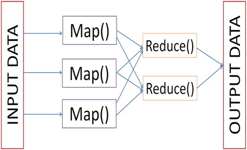
Certain benefits of MapReduce have been highlighted by Ghemawat et al. (2003), Dean and Ghemavat (2008) and Pavlo et al. (2009), in comparison to other parallel database management systems. The former illustrate that MapReduce has a “simplified” functionality with essentially two major functions, namely “Map” and “Reduce” (Figure 1). Non-requirement to follow a certain “schema” for loading data improves its usability. Pavlo et al. (2009) have discussed Google’s implementation of MapReduce at length. They utilize resources and the processing capabilities of Google to use thousands of devices in parallel that are connected via Ethernet. They elaborate on the major enhancement of the indexing system, which is used for the “Google web search service”. The improvements include simplified code and the bypass of glitches due to network or machine failures, since the “MapReduce architecture” is able to account for these.

Figure 1. MapReduce architecture, depicting input data being divided into more manageable chunks, following which a reducer is applied to each of these chunks until it is finally recompiled to give us our output.

As highlighted by Gorelick et al. (2017), GEE uses the MapReduce architecture for parallel-processing or “batch” processing of data. For example, a user would like to calculate the mean EVI value for a certain pixel from a Landsat 5 32-Day EVI collection, over time. The system would start by dividing the complete image collection into separate chunks (“Map” phase), followed by the mean() function being applied on each chunk independently (“Reduce” phase). The final output, which is a single value for the mean, is attained when the independent chunks are recompiled. We discuss this concept in more detail in the “Results and discussion” section, in the context of our research problem and why this proved to be a challenge within the GEE API.

Over the past few years, in addition to the benefits of MapReduce, there has also been a widespread discussion regarding its challenges. A well-known argument presented by DeWitt and Stonebraker (2008) is MapReduce being superficial for handling large-scale and demanding data processing. They strongly debate the need for schemas to avoid the inclusion of low quality or “corrupt” data into the process. Additionally, they also heed importance to indexing, especially in cases where one is calling a filtered collection. This is attributed to the fact that proper indexing may reduce the number of data calls made by the server.

Every database management system has its own pros and cons. Thus, over time, many new approaches to handling big-data have been developed to reach the most efficient solution. The system we explore in this paper is one such approach that attempts to cater to the needs of a growing section of big-data analysts, particularly for EO data. We start by testing this system for Singapore which gives us an insight into the working of GEE.

GEE vs. other big EO data platforms

One of the main advantages of GEE remains the ease-of-use and the consolidated library of global remotely sensed data. Presently, users from a wide variety of disciplines are engaged in projects that have been implemented in GEE, such as, the Hansen global land cover (Hansen et al., 2013) dataset or the Global Forest Watch (2014) of the World Resources Institute. Another major benefit that arises from working with GEE is its cloud computing power. Data processing works well as the personal computer memory of the user is not a limiting factor at any point, especially when working with global-scale data and imagery. However, the availability of an API presents a trade-off between the ease-of-use for a user and the flexibility to implement complex functions within said API. By this we stress on the need for clarity regarding the implementation details of certain raster and vector functions. For example, Interpolate() applies a linear function to each point of each band for a raster or formaTrend(), which calculates the short- and long-term trends in a time series. When running complex transformations, users should be able to manipulate functions and modify them to adapt them to tackle specific problems. Thus, it becomes vital for users to have back-end access in processing platforms.

In most open-source data analysis tools such as SciDB (Brown, 2010) or GeoTrellis (2016), users have access to the source code which enables them to understand commands in detail. However, the back-end computing that takes place in GEE does not allow this. Users are able to share scripts openly within their directories, which makes analysis reproducible in a certain restricted sense. This is only open to the community of beta testers for GEE owing to the proprietary nature of the GEE API. Users are restricted to using the Javascript or Python interfaces available.

Cloud computing platforms provide open access to datasets and analysis. The availability of large amounts of satellite imagery calls for diminishing constraints for sharing data among users, reproducibility of scientific results and targeting extremely specific research problems. Within the last few years, GEE has sought to provide these services to the scientific and nonscientific communities at large.

In contrast to cloud computation programs are stand-alone programs such as, R and Python or cloud architectures such as GeoTrellis. Open-source projects conducted using R and GeoTrellis do tackle the problem of back-end access; however, the ease-of-use across different systems diminishes. For example, the open-source raster data handler GeoTrellis, which is built using Spark, is compatible with Linux. However, setting up the cloud back-end of GeoTrellis is a challenge within itself, especially on other operating systems. Thus, in order to ensure interoperability among datasets, it is essential to allow users test out their algorithms on various data types and across platforms and machines. One such recent example to provide an open-access web-service for users, with an R interface, is the Web Time Series Service (WTSS) (Câmara et al., 2016; Vinhas et al. 2016). The interface of the WTSS in R gives a simpler way to retrieve and manipulate large scale EO data. This is shown in the paper by Vinhas et al. (2016), where the Time Weighted Dynamic Time Warping algorithm is implemented on a Moderate Resolution Imaging Spectroradiometer (MODIS) Normalized Difference Vegetation Index (NDVI) 3D data array.

The island-state of Singapore

The island country of Singapore is located in the Malay Peninsula in Southeast Asia (1°14ʹ N, 103°55ʹ E). The country is made up of 63 islands with a total land area of ~700 km² and a population of 4.4 million (Davison, 2007). Singaporean climate is primarily a “tropical rainforest” climate with fairly steady temperatures, high levels of humidity and abundant rainfall (Lum, Lee, & LaFrankie, 2004; National Parks Board, 2015). The island’s landscape is dominated by man-made structures, a majority being residential and commercial structures (Koh, 2005, 2007), with a blurry distinction between rural and urban landscapes (Kardinal Jusuf, Wong, Hagen, Anggoro, & Hong, 2007).

Land cover distribution of Singapore

More than 50% of the landmass of present-day Singapore is covered by urban structures (Davison, 2007). A majority of the country’s remaining forests (~2000 ha) are protected as reserves. Mainland Singapore is surrounded by smaller islands belonging to its territory, namely the Jurong Island, Sentosa and Pulau Tekong (Figure 2). These smaller islands have been developed on reclaimed land.

Figure 2. The study area, Singapore (1.3521° N, 103.8198° E), highlighting the study areas selected for this preliminary analysis, Tuas industrial zone (red) and Central Catchment Reserve (green). (Source: Open Street Map, 2018).

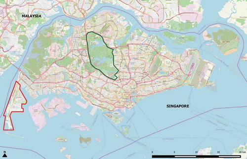
For the purpose of this study, we selected two subregions within Singapore, namely the Tuas industrial zone and the CCR (Figure 2). Our motivation for doing this is due to LULCC being highly localized processes on the island. With strong policies against encroachment and deforestation, observing Singapore as a whole would not yield interesting results as the island has not witnessed extreme land use/cover conversion activities over the past 20 years. Within the last decade, the activity that dominates the island in terms of land change is dredging. This practice is concentrated at the boundaries of Singapore as dredging is used to create additional land space, as opposed to changing the existing land cover profile of the country. We discuss this process in detail in the next sections as well.

Tuas industrial zone

Tuas is an industrial area (area ~20.82 km²) located in the southwest of mainland Singapore (Figure 2). The zone has been developed over the past years on reclaimed land. Land for Tuas was reclaimed primarily through dredging, which involves the depositing sand onto the ocean floor to create “land”. It is the manufacturing hub of the petrochemical and biofuel industry in the country. Future plans for this region include the construction of the Tuas port to handle operations for container vessels at a large scale (Maritime and Port authority of Singapore, 2015).

Central Catchment Reserve

The CCR (area ~44 km²) of Singapore (Figure 2) can be seen mostly in the heart of the city-state. These wetland forests are delineated as a protected area, namely the CCR and the Bukit Timah catchment reserve (Figure 2). This region consists primarily of freshwater swamp forests and patches of lowland forest cover, which was the original primary forest cover of this area (National Environmental Agency of Singapore, 2015). It encompasses the biggest continuous portion of primary rainforest (~70 ha) in Singapore (Davison, 2007; Shono, Davies, & Chua, 2007).

Methodology

In this section, we present an overview of the datasets and software used. We describe some basic functions used within GEE to load data into the GEE API, access uploaded imagery and perform raster overlays. This is followed by the description of the time series analysis of MODIS and Landsat EVI data from years 2006–2010 for the study areas. The methodology is explained with the aim of understanding the computational workflow of GEE. Thus, we selected a simple research problem for a small land area, which offers an important insight into the working of GEE.

Data description

Singapore has a highly urbanized landscape which makes it worthwhile to explore its urban sprawl. This analysis can be deepened by observing the EVI signals of the urban land class for Tuas and the wetland land class that dominates CCR of the city-state (Figure 2). The EVI was chosen over the NDVI and other indices due to its resistance to atmospheric noise. Our study area is located in a tropical area which is heavily affected by clouds and smog from crop burning in Indonesia through year, thus the EVI works more efficiently to counter the effect of haze (Churkina, Schimel, Braswell, & Xiao, 2005; Matsushita, Yang, Chen, Onda, & Qiu, 2007).

Landsat 5 32-Day EVI

The Landsat 5 32-Day EVI product is compiled using the “Level L1 orthorectified” imagery. The values of the EVI range from −1 to +1, measuring greenness over an area. The closer the values are to +1, the more the presence of vegetation.

The formula used to calculate the EVI is

(1)

where, ρ = atmospherically corrected surface reflectance for the blue, red and near infrared bands.

In the GEE database, this product has been corrected for cloud cover. The EVI value for clouds or clouded areas is specified as “masked”. The spatial resolution for this dataset is 30 m.

For our study, we acquired imagery starting 1 January 2006–31 December 2010. The reduced image collection consists of 60 images.

MODIS daily EVI

The MODIS Daily EVI product is based on the red and blue bands of each tile of the MOD09GA MODIS surface reflectance composites. GEE provides this dataset starting 24 February 2000 up to the present year. The spatial resolution for this product is 250 m.

For the purpose of our analysis, we acquired imagery starting 1 January 2006–31 December 2010. The reduced collection contains 1823 images.

MODIS collection 5 land cover type

The MODIS collection 5 land cover type product (MCD12Q1-1) consists of land use classifications with a 500-m spatial resolution (Friedl et al., 2010) representing global tree, herbaceous and bare ground cover. This product is an improvement on the MODIS collection 4 global product. It provides five different classification schemes for each year, namely, “International Geosphere Biosphere Programme”(IGBP), “University of Maryland” classification, MODIS LAI/FPAR, “Biome BGC” and “Plant functional type” (Friedl et al., 2010; Ganguly, Friedl, Tan, Zhang, & Verma, 2010). This paper makes use of the IGBP classification system, which consists of 17 land classes as outlined in Friedl et al. (2010).

Globcover (2009)

This global land cover map has a 300-m spatial resolution to prescribe 22 land classes to classify the globe. The data are based on ENVISAT Medium Resolution Imaging Spectrometer (MERIS) Level 1B imagery. The land classification scheme GlobCover (2009) follows is the Land Cover Classification Scheme developed by the United Nations Food and Agriculture Organization. The validity of the product is from 1 January 2009 to 1 January 2010.

Data processing in GEE

GEE is a platform for processing global-scale satellite imagery dating back up to 40 years (Google Earth Engine, 2012). It allows users to download and upload global satellite imagery, as well as allowing them to perform complex calculations on the same. It comprises of two main components that work in sync with each other, namely, the Google Earth Engine Explorer (EE) (for viewing datasets) and the Google Earth Engine Playground (EEP) (Figure 3(a,b)).

Figure 3. (a) Google Earth Engine Explorer (https://earthengine.google.com/) that is an efficient data visualizer (b) Google Earth Engine Playground (https://code.earthengine.google.com/), which is the JavaScript API for carrying out raster, vector and array operations (Google Earth Engine, 2012).

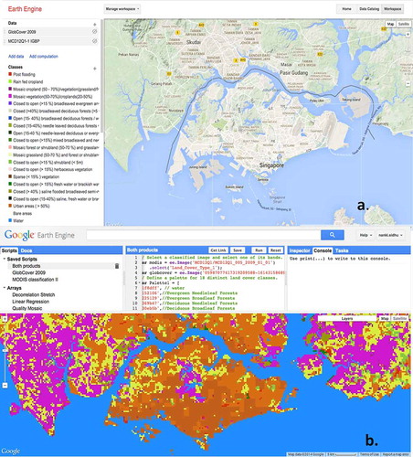
The Google EEP application, a JavaScript API, can be used to load and visualize large satellite imagery and to conduct complex geo-statistical and geospatial operations on our imagery. We use Google EEP to load the “Landsat 5 32-Day EVI Composite”, “MODIS Daily EVI” layers and classified rasters, “MCD12Q1-1 IGBP” and “GlobCover 2009” along with their respective color palettes.

The “MERIS fine resolution full swath level 1B” product is not available in the GEE database. To enable us to access both our classified rasters in the Google EEP, we first upload the original MERIS product into the database via the “Asset Manager”. The uploaded product can then be called from the Google EEP using its “Asset ID”.

Using the Javascript API, we overlay our classified raster imagery and conduct a visual analysis of the classified pixels in both MODIS MCD12Q1-1 and GlobCover(2009). To calculate the number of common pixels from both the rasters, we are able to use the count() function within GEE. Any outputs generated within GEE may be exported to other environments (e.g. R, ArcGIS, QuantumGIS) for further analysis.

Thus, in the exploratory phase, EE and the EEP are effective to visualize the above two products. Using access to the advanced features of the GEE interface, we could create our own classifications for these products. The code used to create these visualizations as well as all other calculations is available in the appendix (Figure A1).

Our aim was to isolate the EVI signal for the two major land classes we observe for this paper and thesis, namely, urban/built up and wetlands (swamp forests). Therefore, for the EVI products, in addition to clipping these collections to Singapore we also filter the complete collections to obtain, years 2009–2012. Out of the list of reducers available in GEE (e.g. mean(), median(), mode(), sum()), we applied the mean() on both, MODIS Daily EVI and LANDSAT 5 32-Day EVI collections. Each pixel in the resultant imagery consists of the value calculated by the reducer, over a specified time period, for a whole collection or a filtered collection. Figure 4. depicts the exact methodological flow of the input and output variables, reducers and functions used within the GEE API.

Generating EVI charts using GEE for land change detection

Through a time series analysis, we are able to look at the changes that occur in the land cover in Singapore over time, focusing on the Tuas and CCR areas. A major benefit of using GEE to conduct our research was the availability of preprepared composites for our time series, thereby not dealing with scanning through collections of raw imagery. One of the main advantages of carrying out a time series analysis as opposed to pixel-based methods is that we are able to assess urban expansion (primary land cover change type in Singapore) and detect otherwise difficult to observe activities such as dredging, which is often a slow process that takes place over several years. The time series analysis was carried out for the whole study areas (Both Tuas and CCR). Furthermore, through the availability of predefined functions, we are able to run our model algebra with relative ease. One of the major challenges we faced while using GEE processing dense time series within the API was to generate a complete and continuous 5-year (or more) time series of our EVI data. This problem in turn revealed the architecture’s incapability of carrying out temporal aggregations as efficiently as spatial aggregations.

To generate a time series for the years 2006–2010, we create a chart for both Landsat and MODIS EVI datasets, with separate series’ representing different years. The inbuilt chart feature was used to construct these time series, using the Chart image series day of year by year function in GEE. GEE chart layouts are similar to the charts plotted in Google spreadsheets and these two systems were found to be well integrated with one another.

The EVI data for both MODIS and Landsat datasets were plotted only for the regions outlining Tuas and the CCR. This was done by clipping the MOD09AEVI and Landsat5 32-Day EVI collections to the spatial polygons seen in Figure 2. One way of trying to further improve the processing speed and time was to also apply a temporal reduction, by sorting the metadata of the imagery according to month and year (Figure A2, Line 17). This was done to generate a CSV file, which is generated by the server and can be stored directly into one’s personal Google Drive. The detailed code can be found in the appendix in Figure A2 (Line 47).

While plotting the observations for the MODIS Daily EVI imagery, we faced many computation time-outs, especially for charting this into a time series. We further observe that there was an increase in the processing time for calculating monthly means from daily values and printing them into a CSV file (Figure A2, Lines 51–54). Upon attempting to plot daily values for more than 6–8 years at a time, the computation timed out. Thus, temporal and spatial manual reductions were needed, in order to break down the processing load.

Another challenge while using GEE was to filter out “zero” values from the EVI products in order to generate an EVI signal. The presence of null values in the data would result in computational errors messages. The value assigned to cloudy pixels in this imagery was “masked”. Thus, we mask the images with themselves, rendering the cloudy pixels transparent and thereby excluding them from our algorithm.

Results and discussions

Singapore has been a hub for urbanization for the past 20 years approximately. The increased construction was captured in the southwestern and the land near the Changi Airport. The CCR is subject to strict laws by the Singapore Land Authority and National Parks. Thus, the forested areas within Singapore have been protected against encroachment for numerous years. Furthermore, being more of a city-scale country, LULCC is strongly controlled by the government highly efficiently.

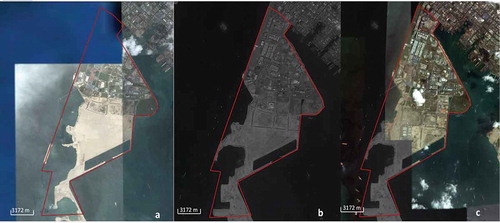
A major challenge of observing spatial and temporal patterns over Singapore is the lack of availability of detailed land cover maps for the country. The most detailed forms of land cover data available are the concept plans devised by the Urban Redevelopment Authority of Singapore (2017); however, as the names suggest, these maps are conceptual and predictive in nature. Hence, we make use of Google Earth imagery, (Figure 5), to analyze the spatial distribution of changes, specifically in Tuas, that we associate to the temporal changes in our EVI time series.

Figure 4. A methodological framework depicting the steps undertaken to generate a spatially and temporally reduced time series of EVI values and measure computational times within the GEE API. The boxes in the right column show the input datasets and variables used throughout the process.

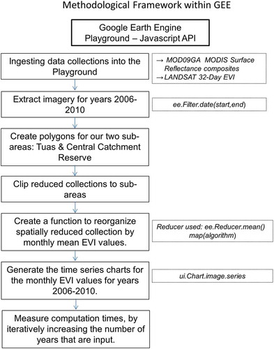
Figure 5. The gradual change in the land cover of the Tuas industrial area (a) 2006, (b) 2008, (c) 2010 (Google Earth, 2015). Also, the activity of dredging through which land is added can be seen over time.

EVI signature for Tuas industrial zone

Rapid industrialization can be seen here since the year 2006 (Figure 5). Conversion can be observed from barren land to built-up area, in a span of over 10 years.

As seen in Figure 6(a), the Landsat dataset contains a lot of missing data values. Google EEP attempts to linearly interpolate missing data points; however, this does not present a true scenario of the urban growth in Tuas. Even though Landsat has a higher spatial resolution than MODIS, it is not as frequently sampled, and thus, does not capture the conversion that took place especially of water into built-up land.

Figure 6. (a) Landsat 5 32-Day EVI signal for Tuas, Singapore for years 2006–2010 (Google Earth Engine, 2012). The gaps in the time series represent the missing data for Singapore on several dates due to severe cloudy and haziness. This also highlights the need for a denser time series for areas that are plagued with this problem of clouds, especially tropical countries in Southeast Asia. (b) The MODIS Daily EVI signal for Tuas, Singapore for years 2006–2010 (Google Earth Engine, 2012). The availability of daily observations, even though the spatial resolution may not be ideal for a certain study area, may provide us with a better view of the land cover variation over long periods of time. The lower EVI values indicate the presence of a rocky terrain and sand, which is the material used for dredging in this area.

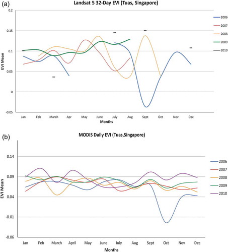
Figure 6(b) represents the urban change, as captured by the MODIS Daily EVI product. Owing to the daily EVI values, the slow and gradual conversion of land is seen quite clearly. Two major lows can be seen in the years 2006 and 2008. In the year 2006, western parts of Tuas had not been converted into land (Figure 5). One of the main methods of expanding the coast in the southwestern part of this area is “dredging”, which is the process of using sand to create “land”. In the Tuas region, approximately 15–20 m of sand or other fillers were used to extend the coastline and utilize this area for industrial construction (Von Mayer, 2005). The top layer of soil in Tuas, consisting of a thin layer of loose sand, is followed by dense and dark clayey soil (Urban land redevelopment authority, 2010). As can be seen in Figure 6(b), values of EVI lie within the 0.05–0.1 range, which indicates the presence of mostly sand and rocky terrain (NASA Earth observatory, 2015). A major phase of the extension of western Singapore, using dredging, was planned for the period 2000–2008 and the seabed in western and southwestern Tuas has been built up using mostly sand (Figure 5). In 2008, one of the major constructions that started around the first quarter of the year was the construction of the Neste biofuel plant, the largest plant of its kind in the world, handling production of 800,000 million tons (approx.) of diesel (per year).

Increasing urban expansion can be seen in Tuas (Figure 5), which may also be ascribed to the construction of two incinerators in Tuas and Tuas South. Western Tuas also developed to accommodate oil barges and tankers. In the years leading up to 2014–2015, Tuas has seen a lot of development and construction, especially the formation of infrastructure for chemical and biofuel industries, and houses manufacturing plants from pharmaceutical and chemical companies.

From Figure 6(b), one interesting observation is the average EVI values in the year 2007 seem higher than those of 2008. This may be explained due to fact that Singapore experienced a record high in rainfall for the years 2004–2007 (Department of Statistics (Singapore), 2016; 2017), indicating the existence of foliage and plant remains among the top soil layer. Higher rainfall leads to the formation of peaty or wet sand/soil which lays the foundation for palm oil production at the biofuel plant.

EVI signature for the CCR

The edge of transition of the wetlands into urban areas is clearly defined. This may be attributed to the extremely strong implementation of the law, which further makes it extremely interesting to observe changes that have occurred on the island. Singapore’s climate is fairly constant all year round, with humid tropical conditions. One interesting feature that affects islands in Southeast Asia is rainfall and typhoon events, especially in the second half of the year. These events may cause vegetation to mimic a pattern of seasonality, which is captured within the EVI signatures, in the form of spikes in the EVI values.

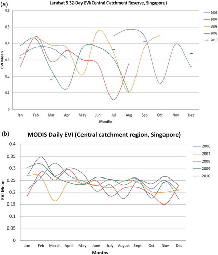
As could be seen with the previous set of results, the Landsat data (Figure 7(a)) consist of a lot of missing values. This is attributed to the small landmass of Singapore and the problem of heavy cloud cover through a majority of the year. Thus, from a dataset with a lot of missing values, it is hard to see the seasonality that gets highlighted in the MODIS dataset. As can be seen in Figure 7(b), EVI values are higher toward the start of a year, indicating more “greenness” in that area at that time. The two main monsoon periods take place are December–March and June–September (National Environmental Agency of Singapore, 2015). Thus, we see the increase in foliage following these periods of heavy rainfall, with values reaching approximately 0.35, around the months of February and September.

Figure 7. (a) Landsat 5 32-Day EVI signal for the Central Catchment Reserve (CCR), Singapore for years 2006–2010 (Google Earth Engine, 2012). (b) MODIS Daily EVI signal for the CCR, Singapore for years 2006–2010 (Google Earth Engine, 2012). We find that the CCR is mostly affected by the monsoon cycles that affect Southeast Asia as a whole, with an increase in greenness following the monsoon periods (December-March, June-September).

GEE: an evaluation

Throughout this paper, we utilize the computing abilities of GEE. All its components (GEE Explorer and EEP) work well together to provide an infrastructure for visualizing, downloading and uploading imagery into the system. The system provides an up-to-date library of 40 years of remotely sensed data. The two main programming languages used in EEP are JavaScript and Python. The official documentation provides helpful examples for users to perform basic and specialized tasks using both APIs. In the following sections, we discuss the strengths and shortcomings of GEE as a cloud computing-based remote sensing platform.

Ease of functionality

Conducting a global, continental or country-scale analysis using alternative programs would take a client a great amount of time and computing resources (Venterino, Schall, & Solichin, 2014). In contrast, owing to the cloud computing capabilities of GEE users are able to visualize the imagery they require in the GEE GUI (Explorer). Imagery retains its “original” spatial reference and metadata. Satellite imagery, namely, the global-level classified product, GlobCover (2009), was initially uploaded using Google Maps Engine (ME); however, we migrated our uploaded imagery to the Asset Manager as Google ME was discontinued in the previous years. This process is efficient while the upload time was ~2 h (518.26 Mb). An important feature of GEE is the use of “fusion tables” to upload vector imagery. Fusion tables are essentially “data tables” that have geometry in a simple feature column, which can be visualized in GEE. These tables can also be used to import and export Keyhole Markup Language(KML)/Keyhole Markup Language Zipped(KMZ) data types. GEE supports a wide variety of data formats and data can be directly downloaded as zip files or exported to Google Drive and used in other remote sensing and GIS platforms.

Processing capabilities

The parallel processing capacity of the GEE infrastructure makes it efficient to run spatial reductions, over image collections (Gorelick et al., 2017). The tile-by-tile processing method of EE applies a spatial (e.g. Median()) reducer to each tile. First, each scene is divided into several tiles, with each tile in turn being sent to the numerous Google servers, to be processed. These servers work in parallel and independently of one another. The result is the “reduced image(s)” which is the outcome of the reconstruction of the tiles. Applying a temporal reducer (filtering through a collection to get specific years) proved to be slightly more challenging. While generating a time series chart for several years, we experienced “memory allocation” or “computational time-out” errors, which we explain in the next section. Examples of the different functions within GEE can be seen in the appendix.

Computational times within GEE

The computational power of GEE is quite high, global-scale imagery can be processed within a matter of minutes. Figure 8 is a depiction of the computation times, while we tested out the code by selecting different number of years with each iteration. As expected, computation times increased with the increase in the amount of data to be processed; however, computational time-outs also came into play after a certain point.

Figure 8. Increase in computation times with increase in the number of years being computed to eventually “time outs”. An increase in number of years leads to an increase in the number of tiles being inputted.

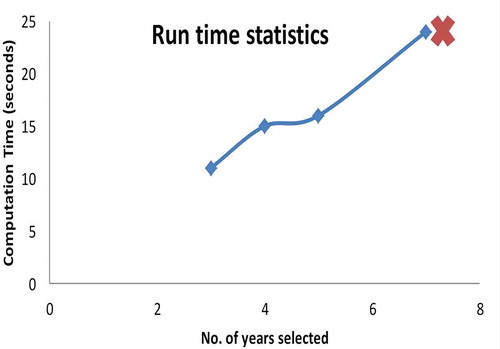
While generating a time series chart for several years, we experienced “memory allocation” or “computational time-out” errors. This may be attributed to the MapReduce architecture that Google adopts for most of the tools and features it offers. Data filtered for dates sort pixels not only spatially but also temporally. A time series may cut across many machines, calling each pixel in time for each machine. Breaking images into chunks of time may make it possible to process over multiple machines. The recompilation of these time chunks may however result in a strain on the servers that presents itself as a limitation of the MapReduce flow in GEE. This challenge can successfully be addressed using the development of databases such as SciDB or the WTSS that strategically organize input data into arrays dedicated for 3D analysis of dense time series’.

Conclusion

Based on the preliminary analysis conducted using GEE, we find that this platform is a powerful tool for analyzing a wide variety of data simultaneously, in one consolidated system. However, supporting both spatial and temporal analysis together is not an obvious task for the platform. Starting out with a small study area, we attempted to test the limits of the system. Based on the frequent computational time-outs despite the small study areas, we find it is of key importance to strategically load and aggregate our input data into GEE, especially to conduct continental and global-scale analysis. The analysis conducted using GEE managed to provide inputs into the urban growth that took place in Tuas for the years 2006–2010 using the MODIS EVI data. The Landsat 5 32-Day EVI data does not yield useful results due to the presence of several missing data values for Singapore. The wide gaps in the data are attributed to the dense cloud cover affecting large parts of Southeast Asia for most months throughout a typical calendar year.

It is of interest to observe how GEE fares against an array-based database management system such as SciDB which focuses strongly on the organization of its input data. As opposed to GEE, SciDB emphasizes on the user being able to select the multidimensional chunk sizes they would prefer to divide their data into, to carry out complex analysis (Stonebraker, Brown, Poliakov, & Raman, 2011). This is done with the aim of reducing computation time, strain on servers and an efficient storage system for big datasets.

The main input of this study is to understand the contribution of big-data repositories to handle large amounts of data. Furthermore, many of these platforms strive to be openly accessible; however, the ease of access varies from platform to platform. For example, platforms like GeoTrellis and SciDB, which consist of manually building a cloud environment, but only on Linux systems, thereby limiting its use for other machines. For the remote sensing community, in addition to data processing and analysis, it becomes essential to efficiently organize and preprocess our imagery, especially when dealing with dense time series’ data. With the run time statistics as depicted in Figure 8, we can see the computation effort increases with an increase in the number of pixels that are used as input for the analysis. As discussed in Câmara et al. (2016), an important point highlighted is the “cost of research friendliness” when it comes to using different web services for organizing remote sensing data. Time series-based analysis forms a strong and important foundation for the detection of long term trends and changes in land use and cover.

In today’s time, when data are becoming denser, especially the availability of the new Sentinel series, users of remote sensing data are looking and exploring more ready-to-use options such as what is offered by Google. Platforms such as these definitely come as an advantage in terms of handling large datasets and creating powerful visualizations. The user friendliness of these platforms also creates appeal among “nonexpert” users of satellite imagery.

Disclosure statement

No potential conflict of interest was reported by the authors.

Appendix

This section contains the code we have used to overlay our MODIS IGBP land cover and GlobCover (2009) classified rasters in GEE. Users are free to adapt this code and reproduce our results, if they are working on similar platforms.

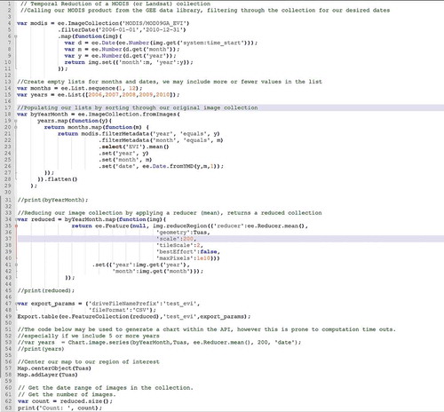
Below is the code we used to conduct temporal reductions on both MODIS and Landsat image collections to generate yearly EVI time series charts using the MODIS Daily EVI and the Landsat 32-Day EVI datasets.

Figure A1. JavaScript code used in the GEE API to explore the handling of classified rasters and raster overlay within GEE.

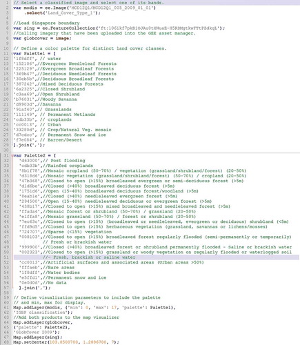
Figure A2. JavaScript code used in the GEE API to generate temporally reduced EVI time series from MODIS Daily EVI and Landsat 32-Day EVI data collections for our study areas Tuas industrial zone and CCR.

References

- Brown, P.G. (2010). Overview of SciDB: Large scale array storage, processing and analysis. In Proceedings of the 2010 ACM SIGMOD international conference on management of data (pp. 963–968). ACM, New York, NY.
- Câmara, G., Assis, L.F., Ribeiro, G., Ferreira, K.R., Llapa, E., & Vinhas, L. (2016). Big earth observation data analytics: Matching requirements to system architectures. In Proceedings of the 5th ACM SIGSPATIAL international workshop on analytics for big geospatial data (pp. 1–6). ACM, New York, NY
- Churkina, G., Schimel, D., Braswell, B.H., & Xiao, X. (2005). Spatial analysis of growing season length control over net ecosystem exchange. Global Change Biology, 11(10), 1777–1787.
- Davison, G. (2007) Urban forest rehabilitation–A case study from Singapore (pp. 171). Keep Asia Green.
- Dean, J., & Ghemawat, S. (2008). MapReduce: Simplified data processing on large clusters. Communications of the ACM, 51, 107–113. doi:10.1145/1327452.1327492
- DeFries, R.S., & Townshend, J.R.G. (1994). NDVI-derived land cover classifications at a global scale. International Journal of Remote Sensing, 15, 3567–3586.
- Department of Statistics, Singapore. (2016). Retrieved December 20, 2016, from http://www.tablebuilder.singstat.gov.sg/publicfacing/displayChart.action
- Department of Statistics, Singapore. (2017). Retrieved January 1, 2017, from http://www.singstat.gov.sg/statistics/visualising-data/charts/annual-growth-in-industrial-production-index
- DeWitt, D., & Stonebraker, M. (2008). MapReduce: A major step backwards. The Database Column. Retrieved April 12, 2015, from https://homes.cs.washington.edu/~billhowe/mapreduce_a_major_step_backwards.html
- Friedl, M.A., Sulla-Menashe, D., Tan, B., Schneider, A., Ramankutty, N., Sibley, A., & Huang, X. (2010). MODIS Collection 5 global land cover: Algorithm refinements and characterization of new datasets. Remote Sensing of Environment, 114(1), 168–182.
- Fritz, S., See, L., & Rembold, F. (2010). Comparison of global and regional land cover maps with statistical information for the agricultural domain in Africa. International Journal of Remote Sensing, 31, 2237–2256.
- Ganguly, S., Friedl, M.A., Tan, B., Zhang, X., & Verma, M. (2010). Land surface phenology from MODIS. Characterization of the collection 5 global land cover dynamics product. Remote Sensing of Environment, 114(8), 1805–1816.
- GeoTrellis. (2016). Retrieved from http://geotrellis.io/
- Ghemawat, S., Gobioff, H., & Leung, S.T. (2003). The Google file system. ACM SIGOPS Operating Systems Review, 37, 29–43. doi:10.1145/1165389.945450
- Global Forest Watch. (2014). World Resources Institute. Retrieved February 6, 2014, from http://www.globalforestwatch.org/
- Google Earth. (2015). Retrieved March 10, 2016.
- Google Earth Engine. (2012). Retrieved February 5, 2014, from https://earthengine.google.org/#intro
- Gorelick, N., Hancher, M., Dixon, M., Ilyushchenko, S., Thau, D., & Moore, R. (2017). Google Earth Engine: Planetary-scale geospatial analysis for everyone. Remote Sensing of Environment 202: 18-27.
- Hansen, M.C., Potapov, P.V., Moore, R., Hancher, M., Turubanova, S.A., Tyukavina, A., … Townshend, J.R.G. (2013). High-resolution global maps of 21st-century forest cover change. Science, 850–853. doi:10.1126/science.1244693
- Kardinal Jusuf, S., Wong, N.H., Hagen, E., Anggoro, R., & Hong, Y. (2007). The influence of land use on the urban heat island in Singapore. Habitat International, 31, 232–242.
- Koh, G.Q. (2005). Singapore finds it hard to expand without sand. PlanetArk. Retrieved September 15, 2014, from http://planetark.com/dailynewsstory.cfm?newsid=30328
- Koh, G.Q. (2007). S’pore tremors raise fear of building on reclaimed land. Reuters (March 2007). Retrieved September 15, 2014, from http://www.wildsingapore.com/news/20070304/070309-5.htm
- Lum, S.K.Y., Lee, S.K., & LaFrankie, J.V. (2004). Bukit Timah forest dynamics plot, Singapore. In Losos, Leigh and Giles Editors (Eds), Tropical forest diversity and dynamism: Findings from a large-scale plot network (pp. 464–473). Chicago: University of Chicago Press.
- Maritime and Port authority of Singapore. (2015). Retrieved June 1, 2015, from http://www.mpa.gov.sg/sites/pdf/sn21/sn21_feature_port-of-possibilities.pdf
- Matsushita, B., Yang, W., Chen, J., Onda, Y., & Qiu, G. (2007). Sensitivity of the enhanced vegetation index (EVI) and normalized difference vegetation index (NDVI) to topographic effects: A case study in high-density cypress forest. Sensors, 7, 2636–2651.
- NASA Earth observatory. (2015). Retrieved from http://earthobservatory.nasa.gov/Features/MeasuringVegetation/measuring_vegetation_1.php
- National Environmental Agency, Singapore. (2015). Retrieved June 1, 2015, from http://www.nea.gov.sg/
- National Parks Board. (2015). Retrieved May 14, 2015, from https://www.nparks.gov.sg/
- Open Street Map (2018). Retrieved on March 13, 2018, from www.openstreetmap.org.
- Parker, D.C. (2002). Agent-based models of land-use and land-cover change. LUCC, Indiana University, USA.
- Parker, D.C., Manson, S.M., Janssen, M.A., Hoffmann, M.J., & Deadman, P. (2003). Multi-agent systems for the simulation of land-use and land-cover change: A review. Annals of the Association of American Geographers, 93, 314–337.
- Pavlo, A., Paulson, E., Rasin, A., Abadi, D.J., DeWitt, D.J., Madden, S., & Stonebraker, M. (2009). A comparison of approaches to large-scale data analysis. In Proceedings of the 2009 ACM SIGMOD international conference on management of data (pp. 165–178). doi:10.1145/1559845.1559865
- Shono, K., Davies, S.J., & Chua, Y.K. (2007). Performance of 45 native tree species on degraded lands in Singapore. Journal of Tropical Forest Science, 19, 25.
- Stonebraker, M., Brown, P., Poliakov, A., & Raman, S. (2011). The architecture of SciDB. In Scientific and Statistical Database Management (pp. 1–16). Springer Berlin Heidelberg. doi:10.1007/978-3-642-22351-8_1
- Urban Redevelopment Authority, Singapore. (2017). Retrieved February 12, 2017, from https://www.ura.gov.sg/sales/TuasSouth21Feb06/tender%20docs/soilrpttuasave2.pdf
- Venterino, R., Schall, M., & Solichin, J. (2014). Google Earth Engine as a remote sensing tool. International Journal of Remote Sensing and Geoscience. Retrieved May 10, 2015, from http://jssolichin.com/remote-sensing/wp-content/uploads/2014/12/Remote-Sensing-Google-Earth-Engine-as-a-Remote-Sensing-Tool.pdf
- Vinhas, L., de Queiroz, G.R., Ferreira, K.R., & Câmara, G. (2016, November 27–30). Web services for big earth observation data. In Proceedings XVII GEOINFO, Campos do Jordão, Brazil.
- Von Mayer, B. (2005). The Writers for hire. Retrieved April 13, 2015, from http://www.dredgebrokers.com/HTML/Dredging/Singapore-Expansion.html