Multi-sensor forest vegetation height mapping methods for Tanzania

ABSTRACT

This paper proposes a new method for mapping of forest cover in Tanzania, in the form of yearly estimates of average vegetation height from time-series of Landsat and ALOS PALSAR satellite images. By using airborne laser scanning data and Landsat-8 data from 2014, a regression between average vegetation height and the specific leaf area vegetation index is established. By using all available Landsat acquisitions of the same area within 1 year, and producing a yearly estimate of vegetation height, the estimation error variance is reduced. The variance is further reduced by Kalman filtering the sequence of yearly estimates. A multi-sensor version of the method comprises application of the radar backscatter when L-band SAR data is available. To conclude, we have demonstrated that estimation of mean vegetation height is possible from dense time series of optical and SAR satellite data. Change detection was able to detect areas with total loss of biomass.

KEYWORDS:

• Specific leaf area index
• cloud masking
• Landsat
• Sentinel-2
• ALOS PALSAR
• airborne laser scanning

Introduction

The current rate of deforestation in tropical regions needs to be reduced in order to decrease CO₂ emissions and preserve biodiversity. Advances in remote sensing methods are needed in order to accurately estimate the state of the forests and how they change over time. For the purpose of tracking biodiversity, ten variables have been suggested by Skidmore et al. (2015): (1) species occurrence, (2) plant traits (including specific leaf area and leaf nitrogen content), (3) ecosystem distribution, (4) fragmentation and heterogeneity, (5) land cover, (6) vegetation height, (7) fire occurrence, (8) vegetation phenology (variability), (9) primary productivity and leaf area index, and (10) inundation.

The Landsat archive provides optical multispectral images in 30 m pixel spacing from 1985 and into the near future. Sentinel-2 was launched in 2015 and provides optical multispectral images in 10 and 20 m pixel spacing and with the same wavelength bands as Landsat-8. Therefore, methods that can estimate essential forest parameters from Landsat and Sentinel-2 are important in an operational system for the measuring, reporting and verification (MRV) of forests in tropical countries, including Tanzania, where the current research was conducted.

It is not immediately clear that vegetation height may be estimated from Landsat images. If a pixel is green, it is difficult to estimate whether the land cover is grass, tall trees or agricultural crops. However, given the seasonal variations in rainy and dry periods that dominate in Tanzania, one may assume that trees are better at preserving their greenness than grass and crops. So, by observing the vegetation repeatedly during 1 year, one may be able to estimate the vegetation height from a dense time series of multispectral optical satellite images such as Landsat and Sentinel-2.

Hansen and Loveland (2012) points out that the recent opening of free access to the Landsat archive, coupled with advances in computing power, means that change analysis will no longer be based on comparison of individual scenes. Rather, automated image pre-processing and land cover characterization methods are needed. Hansen et al. (2013) generate global annual maps of per cent tree cover and forest gain and loss at 30 m pixel spacing from Landsat data for 2000–2012.

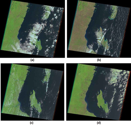
Zhu, Woodcock, and Olofsson (2012) use all available Landsat images to monitor forest disturbance over a 2-year period in a study area in South Carolina and Georgia, USA. The seasonal variation during 1 year is modelled and used to predict the pixel state in the current image, presuming no change in land cover. The predicted value is compared with the actual value to determine if a change had occurred. Three repeated observations are required to confirm a change. However, this method may fail in Tanzania for two reasons. First, in order to model the seasonal variations, the method requires a land cover classification, but this was not available to us. Second, the observed variations in Tanzania are sometimes deviating from a clear seasonal pattern (Figure 1). By comparing four Landsat images of the same area in Tanzania, all acquired in the same month but in different years, one may falsely assume that large areas have been deforested from 1987 (Figure 1(a)) to 1997 (Figure 1(b)). However, only 1 year later (Figure 1(d)), the vegetation suddenly looks more vigorous than in 1987. Then, after another 5 years (Figure 1(d)), the vegetation looks less vigorous than in 1987 and 1998, but more vigorous than in 1997. The reason may be due to varying amounts of rain, or, in occasional years, even lack of rain, in the so-called short rain period, which usually takes place from late November until January.

Figure 1. Four Landsat images of the same area in Tanzania, all acquired in January but in different years: (a) 26 January 1987, (b) 21 January 1997, (c) 24 January 1998, (d) 14 January 2003. False colour images, with Landsat bands SWIR₂ (2220 nm), NIR (830 nm) and red (655 nm) shown as red, green and blue, respectively.

In the present study, the focus was on monitoring the tree vegetation. Although optical images are useful for monitoring the presence of, e.g. plant chlorophyll by computing for example the normalized difference vegetation index (NDVI; see e.g. Aase & Siddoway, 1981; Campbell, 2006; Townshend, Goff, & Tucker, 1985), there is no reliable way to extract forest variables like the forest vegetation height or the biomass directly from a single Landsat image of an area in Tanzania. One strategy could be to use several repeated acquisitions during the same year, and look for seasonal change patterns in, e.g. greenness, dryness, or some vegetation index, in order to learn a statistical relation between seasonal changes and a forest variable of interest. As hundreds of repeated 30 m pixel spacing Landsat acquisitions from 1984 to date are available for all of Tanzania, it seems obvious that this data source must be exploited, possibly in combination with other data sources.

Synthetic aperture radar (SAR) images overcome cloud cover problems, since the radar wavelengths penetrate almost all clouds. SAR images of Tanzania have been acquired in three different wavelengths: X-band, C-band and L-band. Of these, L-band SAR penetrates deepest into the forest canopy and is therefore best suited to estimate biomass (Mitchard et al., 2009) by capturing large tree structures like stems and thick branches which constitute the dominant fractions of the total tree biomass, ignoring low herbaceous vegetation, thin branches and foliage.

Estimation of vegetation height may be done with a variety of remote sensing technologies (Table 1). Airborne laser scanning (ALS) is currently the most accurate method. The laser scanner records the travel time from a pulse is emitted until one or more reflections return to the sensor. With accurate recording of the aircraft’s position and each laser beam’s direction during the scanning, the recorded times may be converted to (x, y, z) positions. If a laser pulse hits a tree canopy that is not too dense, then one part of the pulse may be reflected back towards the sensor, while another part of the laser pulse may continue deeper into the canopy and may even hit the terrain surface before being reflected. A number of reflections from the canopy interior may also occur. Næsset (1997) uses ALS to estimate mean tree height at the stand level, with coefficient of determination R² = 0.94 and root mean square error (RMSE) = 7.7%. The sampling is very sparse, with 15 cm footprint diameter and 3 m average distance between footprints, thus only 0.2% of the area is sampled. However, with improved laser scanner technology, sub-metre sampling distance has been available for more than 10 years. Kwak, Lee, Lee, Biging, and Gong (2007) use ALS to detect individual trees and estimate their heights, with R² = 0.77 and RMSE = 8.2%. Hopkinson, Chasmer, Lim, Treitz, and Creed (2006) use an indirect method to estimate canopy height from ALS data: a regression on the standard deviation of the difference between first and last returns. The R² performance is very good (0.95) but the root mean square error exceeds 10% of the measured mean height.

Table 1. Comparison of previous studies on forest canopy height estimation from remote sensing data.

Authors	Location	Tree species/forest type	Mean height [m]	Sensor	Grid [m]	R^2	RMSE [m]	RMSE [%]
Næsset (1997)	Hedmark, Norway	Pine, spruce	16.2	ALS	Stand	0.94	1.25	7.7%
Kwak et al. (2007)	South Korea	Pine, larch, oak	15.4	ALS	1	0.77	1.27	8.2%
Hopkinson et al. (2006)	Canada	Several forest types	17	ALS	1	0.95	1.80	10.6%
Véga and St-Onge (2008)	Quebec, Canada	Mixed managed forest	23.7	Aerial stereo pairs	0.5	0.96	1.09	4.6%
Lefsky et al. (2007)	Amazon	Tropical with dry season	17.2	ICESat GLAS	60	0.83	4.30	25.0%
	USA	Several forest types	18.9			0.73	5.01	26.5%
Lefsky (2010)	Globally	All forest types	15	ICESat GLAS + Modis	500	0.57	6.50	43.3%
Zhang et al. (2014)	California, USA	Several forest types	35	ICESat GLAS + Landsat	30	0.27	12.33	35.2%
Kellndorfer et al. (2004)	Georgia, USA	Pine plantation	17	SRTM	90	0.79	1.10	6.5%
	Sierra Nevada, USA	Mixed coniferous	17			0.74	4.60	27.1%
Kugler et al. (2014)	Krycklan, Sweden	Spruce and pine, occasional birch	18	TanDEM-X VV	12	0.91	1.58	8.8%
			18	TanDEM-X VV+HH		0.86	2.02	11.2%
	Traunstein, Germany	Spruce, beech, fir	27	TanDEM-X HH		0.8	3.30	12.2%
			27	TanDEM-X VV+HH		0.77	2.80	10.4%
	Mawas, Indonesia	Semi-deciduous peat swamp forest	16	TanDEM-X VV		0.95	1.90	11.9%
			16	TanDEM-X VV+HH		0.69	5.70	35.6%
Lei and Siqueira (2014)	Maine, USA	Several forest types	19.2	Palsar	400 × 800	0.34	3.60	18.8%
Sexton et al. (2009)	North Carolina, USA	Pine	28	ALS	6	0.83	2.22	7.9%
			28	GeoSAR	3	0.7	7.79	27.8%
			28	SRTM	30	0.54	13.42	47.9%
		Hardwood	25	GeoSAR	3	0.38	8.34	33.4%
			25	SRTM	30	0.35	16.39	65.6%
Helmer et al. (2010)	Bahamas	Tropical dry forest	3.5	Landsat time series	30	0.87	0.90	25.7%
Wilkes et al. (2015)	Victoria, Australia	Mixed	18	Landsat+Modis	30	0.58	5.68	31.3%
Wolter et al. (2009)	Minnesota, USA	Hardwood	16	SPOT-5	10	0.69	1.27	7.9%
		Coniferous	17			0.92	1.59	9.4%
Kalacska et al. (2007)	Costa Rica	Deciduous	12	Hyperion	30	0.92	1.10	9.2%
Chopping et al. (2009)	Colorado, USA	Several forest types	7	MISR	250	0.66	3.60	51.4%
Cartus et al. (2012)	Chile	Pine plantations	24	ALS	Stand	0.93	1.70	7.1%
			24	Palsar		0.72	2.75	11.5%
			24	Landsat		0.64	3.23	13.5%
			24	Landsat+Palsar		0.83	2.44	10.2%
Hyyppä et al. (2000)	Kalkkinen, Finland	Boreal	16.5	Airborne C-band SAR	Stand	0.77	2.97	18.0%
			16.5	Airborne hyperspetral		0.47	5.10	30.9%
			16.5	Aerial photograph		0.34	5.43	32.9%
			16.5	Spot multispectral		0.37	5.85	35.5%
			16.5	Landsat		0.26	6.05	36.7%
			16.5	ERS 1-day coherence		0.15	6.43	39.0%

Many authors (e.g., Ioki et al., 2014; Kwak et al., 2007; Lefsky, Keller, Pang, Camargo, & Hunter, 2007) use ALS data to estimate a canopy height model. First, the individual ALS points are classified as one of “ground”, “vegetation”, and, optionally, other classes like “building”, etc. This classification may be done using the TerraScan software (http://www.terrasolid.com). The ALS points labelled as “ground” are used to estimate a digital terrain model (DTM). The ALS first return points of both “vegetation” and “ground” are used to estimate a digital surface model (DSM). A canopy height model is obtained by subtracting the DTM from the DSM.

Although ALS is a direct measurement of terrain and vegetation height, the resulting canopy height model might underestimate the true canopy height (Lefsky et al., 2007). First, since ALS is a sampling technique, the highest locations on individual tree canopies may sometimes be missed, especially with cone-shaped canopies of, e.g. spruce. Second, the terrain surface may be covered by dense understorey vegetation, thus precluding the terrain surface from being sampled, so that the understorey vegetation may be mistaken as the terrain surface.

The main limitation of ALS is that it is cost prohibitive to be applied wall-to-wall for larger territories like the entire territory of Tanzania (945 000 km²), not to mention the need of repeated acquisitions to monitor change. Thus, alternative remote sensing methods need to be investigated.

Véga and St-Onge (2008) use stereo-pairs of aerial images to map historical canopy height models. Image matching techniques are used to estimate DSMs for each of the years 1945, 1965, 1983 and 2003. A recent ALS survey is used to estimate a common DTM. The accuracy is close to that of ALS, and has a huge potential in creating historical records of forest canopy height, given the vast amount of stereo aerial photography in many countries.

Lefsky et al. (2007) use the Geoscience Laser Altimeter System (GLAS) sensor onboard the Ice, Cloud and Land Elevation Satellite (ICESat) to estimate forest canopy height. The method does not need an external DTM. The RMSE = 25% is not as good as with ALS. Another limitation of the method is that the sampling is only along transects. To overcome this, Lefsky (2010) combined ICESat GLAS with Modis 500 m data to produce a global forest canopy height map, but with higher RMSE = 43%.

Zhang et al. (2014) also use ICESat GLAS, but in combination with Landsat. They argue that there is a linear relationship between leaf area index (LAI) and forest canopy height. Thus, by estimating LAI from Landsat data and calibrating with GLAS point observations of canopy height, a continuous forest canopy height estimate is obtained at 30 m resolution, with RMSE = 35%.

Kellndorfer et al. (2004) extracts a DSM from the shuttle radar topography mission (SRTM), which made a global DSM at 90 m grid cell resolution using C-band SAR in interferometric mode. By using the national elevation data of the United States as the DTM, a canopy height model is estimated.

Kugler, Schulze, Hajnsek, Pretzsch, and Papathanassiou (2014) investigate the use of TanDEM-X interferometric SAR for forest height estimation in three different forest types. Two identical satellites with X-band SAR instruments share the same orbit. One is emitting a pulse and both are receiving. From this, a DSM is obtained at 12 m resolution. In single polarization mode, an external DTM is needed. In dual polarization mode (HH+VV), an external DTM is not needed, provided some part of the radar pulse is able to penetrate the forest cover, reach the terrain surface and reflect back to the satellites. In both polarization modes, for about 20% of the pixels, the method is not able to provide an estimate.

Lei and Siqueira (2014) estimate forest height from ALOS PALSAR L-band SAR, using interferometric correlation magnitude, with R² = 0.76 and RMSE = 18.8% for mixed forest in Maine, USA.

Sexton, Bax, Siqueira, Swenson, and Hensley (2009) compare using ALS, SRTM, and airborne X- and P-band SAR interferometry (GeoSAR), for forest canopy height estimation in pine and hardwood forests in North Carolina, USA. The ALS data has 0.5–1.0 m diameter footprints spaced at 4–6 m, which is much coarser than in the ALS studies of Kwak et al. (2007) and Hopkinson et al. (2006). In pine forest, ALS performs much better (R² = 0.83, RMSE = 7.9%) than GeoSAR (R² = 0.70, RMSE = 28%), which again performs much better than SRTM (R² = 0.54, RMSE = 48%). In hardwood forest, the performance was poorer than in pine forest, but GeoSAR (R² = 0.38, RMSE = 33%) is still better than SRTM (R² = 0.35, RMSE = 66%).

Helmer et al. (2010) estimate current vegetation height from a time series of images from Landsat (1984–2003) and EO-1 Advanced Land Imager (ALI) (2005–2006), using a regression model. The independent variables in the regression are the NDMI vegetation index and forest disturbance indicators (undisturbed, goat grazing, cleared for agriculture, and fire disturbance) The R² = 0.87 is good, but RMSE = 25% is high. Wilkes et al. (2015) combine spring and summer Landsat images with a 10 year Modis NDVI time series to estimate forest canopy height in forests in eastern Victoria, Australia, with R² = 0.58 and RMSE = 31.3%. Better results are obtained by Wolter, Townsend, and Sturtevant (2009), who estimate tree height from two SPOT-5 multispectral images with 10 m resolution. They use regression on vegetation indexes and local statistics, obtaining R² = 0.92 and RMSE = 9.4% on a coniferous forest and R² = 0.69 and RMSE = 7.9% on a hardwood forest.

Chopping, Nolin, Moisen, Martonchik, and Bull (2009) estimate forest canopy height from the Multiangle Imaging Spectroradiometer (MISR), which uses four forward and four aft viewing angles in addition to straight down. The results (R² = 0.66, RMSE = 51%) are the least convincing of the studies in Table 1.

Kalacska et al. (2007) estimate canopy height from EO-1 Hyperion satellite data with 220 hyperspectral bands at 30 m grid spacing, acquired over a deciduous forest in the dry season. Regression is done on predictors extracted from wavelet decomposition, and has a better coefficient of determination (R² = 0.92) than regression on a single vegetation index (R² = 0.66).

Cartus, Kellndorfer, Rombach, and Walker (2012) compare using ALS, PALSAR, Landsat-7, and a combination of PALSAR and Landsat for canopy height estimation in pine plantations in Chile. Using PALSAR data from several dates in a single year (2007), with single (HH) and dual (HH+HV) polarization and interferometric coherence, R² = 0.72 and RMSE = 11.5% are obtained. By including three cloud-free Landsat acquisitions from 2005–2007, this is improved to R² = 0.83 and RMSE = 10.2%. Using Landsat alone results in R² = 0.64 and RMSE = 13.5%.

Hyyppä et al. (2000) compare stand-level mean height estimation using different airborne and satellite sensors. Of these, airborne C-band full polarimetric SAR performed best, with R² = 0.77 and RMSE = 18%. For the optical data, airborne hyperspectral data with 30 channels and 2 m resolution performed best, R² = 0.47 and RMSE = 31%. Despite different resolutions, Spot multispectral satellite images with 20 m resolution and three channels, green, red, and near-infrared, performed equally well (R² = 0.37, RMSE = 35%) as scanned aerial photographs in 0.85 m resolution and the same three channels (R² = 0.34, RMSE = 33%). However, Landsat 30 m resolution performed slightly worse (R² = 0.26, RMSE = 37%) despite having more spectral bands. The ERS-1/2 tandem mission provided interferometric C-band SAR acquisitions with 1 day time difference. From these data, coherence images at eight different date pairs, each with 1 day lag, were used, but gave poor results, R² = 0.15 and RMSE = 39%.

To summarize, for ALS, the coefficient of determination, R² varies between 0.77 and 0.95 with RMSE between 7.1% and 10.6%; Landsat, R² 0.26–0.87 with RMSE 13.5–36.7%; Palsar, R² 0.72–0.76, RMSE 11.5–18.8%; other satellite sensors/combinations, R² 0.15–0.92, RMSE 6.5–51% (Table 1). The large variations in R² and RMSE are in part due to the different sizes of the study sites, which range from a single forest plantation to, e.g. the entire state of California, USA. In many of the studies, a canopy height model from ALS data is used as the true values instead of field data.

In this study, we hypothesized that it should be possible to produce yearly estimates of average vegetation height at 30 m pixel spacing from a time series of Landsat and ALOS PALSAR data. The objective was therefore to develop such a method that could be applied operationally over large areas of tropical forests. For calibration of the method, we use ALS data with 1.8 first returns per square metre on average to estimate a canopy height model at 1 m pixel spacing. When aggregated to 30 m pixel spacing, this is regarded as exact measurements of mean vegetation height.

To reduce noise and to provide estimates for areas that have not been observed due to cloud cover, some sort of smoothing may be needed. Since we do not want coarser resolution than 30 m, smoothing in the spatial domain should be avoided. Two popular methods for smoothing in the time domain is Kalman filtering (Kalman, 1960) and hidden Markov model. Salberg and Trier (2011, 2012)) have used a hidden Markov model for temporal analysis of tropical rain forest in Brazil. However, by using the same approach in Tanzania, the seasonal fluctuations of the optical signal may falsely be interpreted as state changes in a hidden Markov model. Kleynhans et al. (2011) used extended Kalman filtering on an NDVI time series for land cover change detection.

Data

Study areas

Two study areas were included: Liwale and Amani (Figure 2). Liwale is representative for 90% of Tanzania, while Amani was included as an extreme case in order to explore the limitations of the proposed method.

Figure 2. The location and extent of the two study areas, shown on a map of Tanzanian district boundaries. The 100 km grid lines are in UTM zone 37 S.

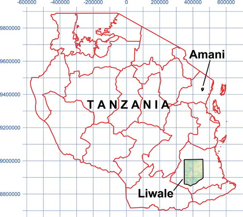
The Liwale study area (S9°54ʹ, E37°38ʹ) covers 15,867 km² of Miombo woodlands with altitudes in the range 150–900 m above sea level and is located in the Lindi region, southern Tanzania. Miombo woodlands cover 90% of Tanzania. As described by Mauya et al. (2015), the rainfall pattern in Liwale is bi-modal with a dry season from June to October. A short rainy period usually starts in late November and lasts until January. There is a dry spell in February followed by a longer wet season which lasts from March until May. Mean annual rainfall is 800 mm.

The Amani study area (S5°08ʹ, E38°37ʹ) covers 127 km² with altitudes in the range 200–1150 m above sea level. It includes the 83.6 km² Amani Nature Reserve, which is a tropical submontane rainforest. The Amani area is located in the East Usambara Mountains, which are parts of the Eastern Arc Mountains in eastern Tanzania. In this forest ecosystem, rain falls throughout the year with two wet seasons, April to May and October to November, and the area receives around 2000 mm rainfall per year (Hansen, Gobakken, Bollandsås, Zahabu, & Næsset, 2015).

ALS data

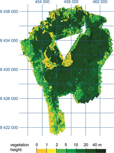
ALS data were collected by TerraTec AS, Norway, in 2012 for both Liwale and Amani, and repeated in 2014 for Liwale (Table 2). The ALS data in Liwale (Figure 3) were collected along 1.4 km wide and parallel strips in a systematic design at 5 km intervals, i.e. there was a gap of 3.6 km between neighbouring strips. A 113 km (east-west) × 156 km (north-south) area was covered with 34 strips in the east-west direction. The repeat acquisition in 2014 was done along the same strips to allow for change analysis. The ALS data in Amani (Figure 4) covered 127 km² wall-to-wall, including a protected high-biomass montane tropical rain forest with some trees taller than 50 m. This area is not typical for Tanzania, but represents an extreme situation with rain forest. The data were collected on six dates in January–February 2012.

Table 2. Airborne laser scanning parameters.

	ALS campaign
	Amani 2012	Liwale 2012	Liwale 2014
Laser scanner	ALS70, snr 7160	ALS70, snr 7160	ALS70, snr 7204
Elevation over terrain	800 m	1200 m	1200 m
Flying speed	135 knots	150 knots	150 knots
Laser pulse frequency	339 200 Hz	193 200 Hz	193 200 Hz
Point density	10.6/m^2	1.8/m^2	1.8/m^2
Field of view	± 16 degrees	± 27.5 degrees	± 27.5 degrees
Acquisition dates	19 January–3 March	10 February–7 March	18 July–8 August
Strip width	459 m	1374 m	1374 m
Strip overlap	20%	N/A	N/A
Strip gaps	N/A	3626 m	3626 m

Figure 3. ALS normalized digital surface model (nDSM), i.e. vegetation height, for Liwale. The 25 km grid lines are in UTM zone 37 S.

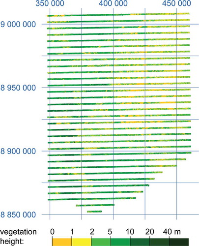
Figure 4. ALS normalized digital surface model (nDSM), i.e. vegetation height, for Amani. The 2 km grid lines are in UTM zone 37 S.

From each ALS data set, average vegetation height was computed on the 30 m Landsat grid. In the ALS data, each ALS pulse had been labelled with class (“ground” or “other”) and return number. From all “ground” returns, a DTM was created at 1 m pixel spacing. From all the first returns, a DSM was created at the same pixel spacing. By subtracting the DTM from the DSM, a normalized DSM (nDSM) was obtained, which may be used as an estimate of vegetation height. By aggregating this to the 30 m pixel spacing Landsat grid, the resulting average vegetation height map is regarded as exact for the purpose of developing a method to estimate average vegetation height from satellite images with 30 m pixel spacing. However, there is a potential problem with the 2014 ALS data in Liwale, since it was acquired in the dry period, which may allow the ALS pulses to penetrate more into the canopy before the first returns occur. Field work conducted at the times of the ALS campaigns (Ene et al., 2017) gave an estimated biomass loss in the range 0.11–0.35Mg/ha from 2012 to 2014, depending on which estimator was used. None of these changes are statistically significantly different from 0 at the 95% confidence level. Therefore, we will scale the 2014 nDSM by a factor (Table 3) to obtain the same mean value as the 2012 nDSM.

Table 3. Computation of scale factor for 2014 nDSM of ALS strips in Liwale.

Number of overlapping 30 m pixels	4,489,466
Mean 2012	5.219 m
Mean 2014	4.621 m
Mean difference	0.598 m
Scaling factor for 2014 nDSM	1.13

Landsat satellite data

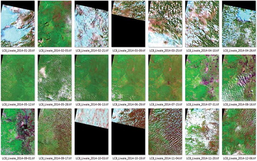
Landsat-4 and -5 data in 30 m pixel spacing were collected for 1984–2011. Landsat-7 data were collected for 1999–2014; after 31 May 2003 the data contained stripes of missing data (SLC-off). Landsat-8 data were collected for 2013–2014. For the period 19 December 2014–13 March 2015, Landsat-8 thermal bands were not available. Only Landsat data that were terrain corrected (level 1 terrain corrected, L1T) were used; thus, a number of acquisitions that were geocoded but not terrain corrected (level 1 geocoded, L1G) were discarded from the analysis (Table 4). Landsat-8 data of Liwale (Figure 5), extracted from path 166, rows 66–67 from 21 different dates in 2014 were used for method calibration together with the 2014 ALS nDSM from the same area. During 2014, the spectral signatures, the number of cloud free observations, and the actual dates of cloud free observations vary over the Liwale study area (Figure 5).

Table 4. Number of Landsat L1T acquisitions of path 166, rows 066–067 used in the study. On some dates, only one of the images (166/066 or 166/067) was available; in such cases, a sum of three numbers is shown. E.g., 3 + 1 + 2 means that three acquisitions of both 166/066 and 166/067 exist, then one of 166/066 only, and two of 166/067 only.

						Excluding SLC-off		Including SLC-off
Year	Landsat-4	Landsat-5	Landsat-7 SLC-on	Landsat-7 SLC-off	Landsat-8	Total L1T	Rejected L1G	Total L1T	Rejected L1G
1984		0 + 0 + 2				0 + 0 + 2	0 + 2 + 0
1985							1
1986		2 + 1 + 5				2 + 1 + 5	4 + 5 + 1
1987		0 + 0 + 1				0 + 0 + 1	2 + 2 + 0
1988	0 + 0 + 1					0 + 0 + 1	0 + 1 + 0
1989	1 + 0 + 1	0 + 0 + 1				1 + 0 + 2	0 + 1 + 1
1990		2 + 1 + 1				2 + 1 + 1	0 + 0 + 1
1991		3 + 0 + 1				3 + 0 + 1	2 + 1 + 0
1992		1				1
1993		4 + 0 + 2				4 + 0 + 2	0 + 1 + 0
1994		3 + 0 + 4				3 + 0 + 4	0 + 1 + 0
1995		3 + 0 + 2				3 + 0 + 2	5 + 2 + 1
1996		1 + 0 + 1				1 + 0 + 1	2 + 1 + 0
1997		3 + 0 + 4				3 + 0 + 4	4 + 3 + 0
1998		4 + 0 + 4				4 + 0 + 4	5 + 2 + 0
1999		2	3 + 1 + 1			5 + 1 + 1	1
2000		0 + 1 + 1	7 + 4 + 3			7 + 5 + 4	0 + 1 + 1
2001			8 + 4 + 2			8 + 4 + 2
2002			7 + 5 + 1			7 + 5 + 1
2003		1 + 0 + 1	4 + 1 + 0	1 + 3 + 1		6 + 4 + 2	0 + 0 + 1	6 + 4 + 2	1 + 0 + 2
2004		3 + 2 + 1		5 + 2 + 3		8 + 4 + 4	3 + 1 + 1	8 + 4 + 3	3 + 2 + 3
2005		2 + 0 + 1		7 + 2 + 5		9 + 2 + 6	2	9 + 2 + 6	2 + 2 + 2
2006		7 + 2 + 2		5 + 4 + 2		12 + 6 + 4	5 + 2 + 2	12 + 6 + 4	5 + 2 + 5
2007		2 + 2 + 0		6 + 2 + 2		8 + 4 + 2	3 + 0 + 2	8 + 4 + 2	3 + 0 + 5
2008		6 + 0 + 5		8 + 2 + 3		14 + 2 + 8	4 + 4 + 1	14 + 2 + 8	5 + 5 + 3
2009		5 + 0 + 1		8 + 5 + 3		13 + 5 + 4	1 + 1 + 0	13 + 5 + 4	1 + 2 + 6
2010		2 + 1 + 1		4 + 2 + 2		6 + 3 + 3	4 + 1 + 0	6 + 3 + 4	4 + 1 + 2
2011		2 + 1 + 0		5 + 3 + 1		7 + 4 + 1		7 + 4 + 1	1 + 0 + 3
2012				9 + 4 + 2				9 + 4 + 2	0 + 1 + 5
2013				8 + 6 + 2	13 + 2 + 0	13 + 2 + 0	0 + 0 + 1	21 + 8 + 2	4 + 1 + 7
2014				11 + 9 + 1	15 + 3 + 3	15 + 3 + 3	0 + 3 + 3	26 + 12 + 4	1 + 4 + 11

Figure 5. Landsat-8 data for Liwale for 20 January–6 December 2014, extracted from path 166, rows 066–067. False colour images with the same bands as in Figure 1. For six of the dates, either path/row 166/066 or 166/067 was not terrain corrected, and thus rejected, resulting in 15 complete extracts,3 partial extracts of the northern part (166/066), and 3 partial extracts of the southern part (166/067); this is indicated in Table 4 as 15 + 3 + 3 for Landsat-8 in 2014.

ALOS PALSAR data

Level-1.1 data from the Phased Array type L-band Synthetic Aperture Radar (PALSAR) onboard the Advanced Land Observing Satellite (ALOS) were acquired from JAXA through the Global Forest Observation Initiative and ESA category-1 proposal no. 27,689. The data gave us full coverage of our regions of interest in Liwale and Amani for each year of the period 2007–2010 with fine beam dual polarization data (FBD) in HH and HV polarization with satellite path numbers 566, 567 and 568.

The level-1.1 data have been processed, i.e. geocoded, radiometrically corrected, including slope correction, with Norut’s in-house developed SAR pre-processing system GSAR (Larsen, Engen, Lauknes, Malnes, & Høgda, 2005) into the same 30 m pixel size grid as the Landsat data.

Methods

The overall goal of the proposed method is to estimate forest vegetation height all over Tanzania, despite obvious challenges due to the following:

1. Varying cloud cover. It is very rare that a single Landsat image is entirely cloud free.

2. Seasonal variations. The yearly cycle usually has two rain periods and two dry periods. However, these vary in length, intensity and spatial distribution from year to year.

3. Saturation. The method may underestimate the vegetation height when the true average vegetation height is above some limit.

The approach to arrive at a general method is as follows:

1. Establish a method that works for the Landsat data that overlaps the ALS area in Liwale, for the same year (2014).

2. Modify the method so that it may be used for Landsat data that overlaps the ALS area in Liwale, from any year.

3. Extend the method so that it may be used for Landsat data everywhere in Tanzania.

The Amani area is not used for method calibration, but is included in the evaluation as an odd case.

The method is novel in the following aspects. (1) It uses all available Landsat acquisitions. (2) It provides vegetation height estimates for all years in the time series. (3) It may be extended to include data from other satellite sensors; this is demonstrated by including PALSAR data.

Processing steps

The proposed method has the following processing steps:

1. Cloud masking of each Landsat acquisition, by using Fmask (Zhu, Wang, & Woodcock, 2015).

2. Compute SLAVI vegetation index (Lymburner, Beggs, and Jacobson (2000).

3. Collect all SLAVI maps of the same area (same Landsat path/row) within the same year.

4. Estimate average vegetation height as a yearly estimate per pixel.

5. Reduce noise by per-pixel Kalman-filtering of the time series of yearly height estimates.

6. Compute change maps (height change estimates per pixel).

Vegetation height from Landsat images

There is a linear relationship between LAI and forest canopy height, provided the forest canopy is not closed or nearly closed (Zhang et al., 2014). We used the specific leaf area vegetation index, SLAVI, (Lymburner et al., 2000) as an estimate of LAI. SLAVI uses three Landsat bands. The index uses the positive correlation of leaf chlorophyll with the NIR band, and the negative correlation with the red band. In addition, the short wave radiation is absorbed by leaf water content, and the effect is stronger in the SWIR₂ band (2.2 µm) than in the SWIR₁ band (1.6 µm). SLAVI is calculated by

Compared with other vegetation indices like NDVI and NDMI (Jin & Sader, 2005), SLAVI is less affected by cloud shadows, which may remain even after cloud and cloud shadow masking.

In order to establish a relationship between SLAVI and forest canopy height, the nDSM with 30 m pixel spacing from the 2014 ALS data from Liwale were used together with SLAVI maps from all 21 Landsat-8 acquisitions from 2014 of the same area. The normalized DSM (nDSM) provides an estimate of the vegetation height. The nDSM was aggregated to the 30 m Landsat grid, thus providing an average vegetation height within each Landsat pixel. After the scaling of the 2014 nDSM, as described above, it was regarded as an exact measurement of mean vegetation height for each Landsat pixel.

In order to investigate if there is a relationship, which may be used in regression, between SLAVI and vegetation height, the following plot was made. The SLAVI axis was divided into bins of width 0.1. Then, for each Landsat-8 image from 2014, only the cloud-free pixels that had a mean vegetation estimate from the 2014 nDSM of Liwale were used. Of these, for all pixels within one SLAVI bin, the average of the nDSM vegetation height estimates for those pixels was used. This was repeated for all SLAVI bins. This resulted in the 21 curves in Figure 6, with one curve for each Landsat acquisition date.

Figure 6. Mean vegetation height plotted for 0.1 SLAVI bins. Each curve is for one Landsat image, labelled “average-<day-number>”.

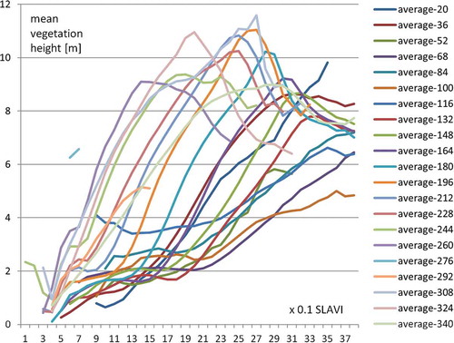
For each curve (Figure 6), there appeared to be a near-linear relation up to a peak. Beyond the peak, the relation seemed to be near-linear with a negative slope. However, by closer inspection of the scatter plots of the data (Figure 7), there was only a small fraction of data points beyond the peak. Thus, this part of the curve may be ignored. Scatterplots of SLAVI versus vegetation height for each of the 21 Landsat images (e.g. Figure 7) also indicated that there may be a linear relation between SLAVI and vegetation height for most of the images, but also that the variance is high.

Figure 7. Scatterplot of SLAVI vs. ALS vegetation height for Landsat-8 data of 15 July 2014. Colour codes: white 0–1, Darkest blue 2, yellow 50, red 100, darkest red 140–1835. The solid black line is the same as the orange line labelled “average-196” in Figure 6, i.e. the mean vegetation height for any given 0.1 SLAVI bin. The dashed and dotted lines are the mean plus and minus one standard deviation, respectively.

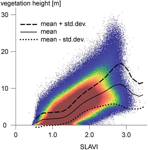
Table 5. Regressions between Landsat SLAVI and ALS vegetation height for Liwale, 2014. ¹Individual regressions for each Landsat image. ²Simultaneous regression with common constant but individual regression slopes.

			Separate regressions				Simultaneous regression
Date	Day	#cloud free	Regression constant^1 a	Regression slope^1 b	R^2	RMSE	Common constant^2 a0	Regression slope^2 b	R^2	RMSE
2014–01-20	20	83,274	−4.00	4.10	0.52	2.34	−3.40	3.80	0.52	2.35
2014–02-05	36	2,652,979	−4.71	4.86	0.44	3.22	−3.40	4.27	0.44	3.23
2014–02-21	52	0
2014–03-09	68	223,516	−2.20	2.10	0.23	2.32	−3.40	2.53	0.23	2.33
2014–03-25	84	161,719	−1.42	2.47	0.23	2.71	−3.40	3.24	0.23	2.75
2014–04-10	100	340,458	−0.49	1.68	0.07	3.16	−3.40	2.72	0.07	3.22
2014–04-26	116	389,276	0.84	1.84	0.08	3.58	−3.40	3.48	0.08	3.69
2014–05-12	132	3,597,385	−5.57	4.17	0.27	3.33	−3.40	3.33	0.27	3.34
2014–05-28	148	1,558,161	−4.95	4.32	0.33	3.08	−3.40	3.64	0.33	3.09
2014–06-13	164	3,954,445	−6.27	5.47	0.44	2.86	−3.40	4.11	0.44	2.91
2014–06-29	180	4,085,720	−5.92	6.12	0.48	2.89	−3.40	4.78	0.48	2.93
2014–07-15	196	4,430,895	−5.48	6.90	0.53	2.86	−3.40	5.65	0.53	2.90
2014–07-31	212	4,516,253	−3.98	6.78	0.49	3.01	−3.40	6.38	0.49	3.01
2014–08-16	228	3,432,935	−2.22	6.17	0.44	2.93	−3.40	7.08	0.44	2.96
2014–09-01	244	4,322,941	−1.96	7.25	0.34	3.29	−3.40	8.60	0.34	3.36
2014–09-17	260	1,821,464	−2.08	8.85	0.24	3.52	−3.40	10.37	0.24	3.60
2014–10-03	276	0
2014–10-19	292	331,082	−0.32	3.82	0.09	1.70	−3.40	8.03	0.09	1.81
2014–11-04	308	1,905,920	−0.81	6.70	0.26	3.69	−3.40	9.19	0.26	3.80
2014–11-20	324	504,222	−2.72	8.19	0.36	3.51	−3.40	8.82	0.36	3.61
2014–12-06	340	2,433,464	−1.23	4.65	0.36	3.51	−3.40	5.95	0.36	3.75

For each Landsat acquisition during 2014, a regression between SLAVI (based on Landsat-8 bands 4, 5 and 7) and the acquired ALS vegetation height was established (Table 5, columns 1–5):

where y is vegetation height, x is SLAVI, a is the y axis intercept at x = 0 (a theoretical vegetation height for SLAVI = 0) and b is the slope of the linear relationship. However, when we encounter Landsat images for other years, with no ALS data available, it is difficult to estimate both a and b. It would be better to have a fixed a = a₀, so that only one parameter, b, needs to be estimated for each new image. This was achieved by the simultaneous regression

Here, a₀ is the common y-axis intercept at x = 0 that all the regression lines run through, b_i, i = 1… N are the slopes of the N regressed lines. In our case, N = 21, as we have Landsat-8 images from 21 different dates in 2014. For each image i, we collected the vegetation height and SLAVI values into the column vectors and , respectively.

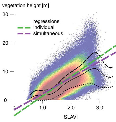
The simultaneous regression (Table 5, columns 8–9) gives a common regression constant a₀ = −3.40. There is no direct physical interpretation of this value; a negative vegetation height is not possible in reality. For each of the N = 21 Landsat-8 images of 2014, the two regression lines may be compared visually with the scatter plot (Figure 8). The simultaneous regression gives a slight increase in root mean square error (Table 5, column 7 vs. 11).

Figure 8. The two alternative regression lines for 15 July 2014 superimposed on the scatter plot.

For a new image k, from another year than 2014, we do not perform a regression between an ALS canopy height model and the SLAVI values, as the true vegetation height values may deviate substantially from the 2014 ALS estimate, especially if there is a substantial number of years between the image acquisition and the ALS acquisition. Instead, we wanted to use the regression

Here, the regression slope b_k is unknown. However, by comparing the new image k to a reference image r, the regression slope was estimated as

where b_r is the regression slope of a reference image of the same Landsat path/row, and µ_r and µ_k are the mean values of the simultaneously cloud-free pixels of the reference image and the new image, respectively. For example, if the new image k has a mean SLAVI value of only half of that of the reference image r, then the regression slope b_k of the new image k will be twice the slope b_r of the reference image. The effect is a data scaling, but with a common offset (regression constant). An alternative approach could have been to use a common regression slope and change the regression constant for each new image. This would have been a data shift, i.e. a_k = a_r + (µ_r–µ_k).

The reference image must be almost cloud free to allow for a large number of simultaneously cloud free pixels. To establish a new reference image for another Landsat path/row, the corresponding regression slope was estimated using the same estimator, but with the mean values estimated for all cloud free pixels in each image. By cloud free, we mean that Fmask has labelled them as valid, and not any of: cloud, cloud shadow, water region, or outside image.

For each image of the same Landsat path/row within 1 year, the regression slope and then the vegetation height for all cloud free pixels were estimated. The yearly average for each pixel was obtained by computing the mean value of the height estimates for all cloud free observations of that pixel within the year. The number of cloud free observations of each pixel was stored in a separate image for later use by the Kalman filtering.

The Kalman filtering requires estimates of the variance associated with the yearly average vegetation height estimates. For 2014, we have measurements of average vegetation height, µ_i, for pixels i = 1, …, I. For each pixel i, we have N_i cloud-free satellite measurements y_ij in the same year, j = 1, … N_i. The yearly average of the average vegetation height for pixel i is

The N_i measurements y_ij of pixel i are not independent. We model this as

where µ_i is the true value, ε_i is the dependent part of the measurement error and ω_ij is the independent part of the measurement error. We will use σ² and τ² to denote the error variances:

For the yearly estimate for pixel i, we then have

This means that we may reduce the variance of by adding more observations (i.e. increasing N_i), but also that we will never get rid of σ². However, this estimate of σ² is a worst-case estimate. To estimate σ² and τ² we use

where is the total number of observations and is the number of pixels for which we have true values . For the 2014 data, this gives and a worst-case estimate of , which gives (Table 6). This means that a large number of observations within 1 year has a limited effect on reducing the estimated variance given by . However, for the purpose of Kalman filtering, the estimated variance (per pixel) is used to indicate to what extent the new observations are to be trusted. We want to differentiate more between few and many observations, and do this by reducing the estimate for σ² and increasing the estimate for τ². We suggest to use , which may better reflect the added value of having more observations within 1 year.

Table 6. Dependent and independent variances of vegetation height estimated from repeated Landsat acquisitions.

Total number of observations, N	41 466 327
Number of ALS measurements, I	4 599 924
Total variance, τ^2+σ^2	10.26 m^2
Dependent variance, σ^2	8.05 m^2
Independent variance, τ^2	2.21 m^2
Mean value of mean vegetation height estimated from 21 Landsat images	5.36 m
Mean value of ALS measured mean vegetation height	5.23 m
Deviation of mean	0.13 m

Vegetation height from PALSAR images

Vegetation height was also estimated for L-band PALSAR data for the years 2007–2010. SAR volume scattering increases with vegetation and it has been shown that there is an exponential-like relationship between SAR backscatter and aboveground biomass (Mitchard et al., 2009). It is therefore reasonable to assume that there is also an exponential-like relationship between backscatter and vegetation height. In order to calibrate this relationship in our data, the ALS data were aggregated to the pixels of the ALOS PALSAR mosaic. In order to reduce for speckle effect, the average ALOS PALSAR mosaic over the 2007–2010 period was aggregated into 90m resolution pixels.

For each 1 m vegetation height bin, 0–1 m, 1–2 m, …., 24–25 m, the average PALSAR backscatter in HH and HV polarization and their standard deviation where calculated. An exponential regression line was then fitted (Figure 9).

Figure 9. PALSAR backscatter versus ALS vegetation height. Exponential regression lines (solid lines) were fitted to the data points (cyan symbols for HV and purple symbols for HH polarization).

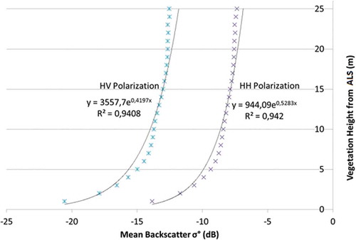
For HH polarization the regression model was with R² = 0.9408. For HV polarization, the regression model was with R² = 0.9420. These regression models were used to estimate the vegetation height for each year 2007–2010 individually in 90 m pixel spacing. The results based on HH and HV polarization individually were then averaged for a final combined result. Finally, it was resampled in 30 m pixel spacing by bilinear interpolation for comparison with the Landsat estimated vegetation heights.

The Kalman filter (described below) required a variance estimate for the PALSAR-derived vegetation height, and may also use a gain factor. The variance and deviation from the mean were estimated for each year individually (Table 7) by comparing with the ALS nDSM height for 2012. The overlap between PALSAR and ALS nDSM coverage was 4,585,781 pixels.

Table 7. PALSAR estimates of vegetation height for 2007–2010 versus ALS measurements for 2012.

	2007	2008	2009	2010	Average
Mean ALS vegt. height 2012					5.203 m
Mean PALSAR vegt. height	5.804 m	5.718 m	5.340 m	5.311 m	5.543 m
PALSAR deviation of mean	0.601 m	0.515 m	0.137 m	0.109 m	0.818 m
Kalman gain factor	1.115	1.099	1.026	1.021	1.065
Variance	10.301 m^2	8.222 m^2	7.785 m^2	7.629 m^2	8.484 m^2

We observe that there was a declining vegetation height trend through the 4 years. As the 2010 vegetation height mean value is reasonably close to the ALS-derived mean value, and closest in time to the 2012 ALS data, it seems reasonable to use the 2010 PALSAR data in order to estimate the variance of the mean vegetation height predictions from PALSAR.

This variance will be used as input to the Kalman filtering (below). The Kalman filtering also requires a gain factor. As the estimated Kalman gain factor for 2010 was close to 1.0 (Table 7), we used the value 1.0 in the subsequent analysis. This was also in agreement with the declining trend of the average vegetation height, i.e. the mean of the vegetation height was expected to be slightly reduced from 2010 to 2012.

Reducing noise

The vegetation height estimates from individual years may vary substantially, given the varying number of satellite observations within each year, and the varying cloud cover in Landsat images. In order to reduce fluctuations in the estimated vegetation height that are not caused by actual changes in vegetation height due to regrowth/growth and anthropogenic or natural losses of trees and other vegetation, but related to biophysical response of the vegetation to the variability in climatic conditions, Kalman filtering was applied. We assume no change as the normal situation, i.e. regrowth/growth is balanced by anthropogenic or natural losses of trees and other vegetation.

The Kalman filtering was designed so that it may accept any of the following four situations for each year in the sequence:

• No data

• Estimate from Landsat

• Estimate from PALSAR

• Estimate from both Landsat and PALSAR

The Kalman filter was used to model a sequence of process states. The process state y_k+1 at time t_k+1 is dependent on the state y_k at a previous time t_k:

where F is the change factor and w_k ~ N(0,Q) is the process noise, assumed to be normally distributed with zero mean value and variance Q. The observation x_k at time t_k is:

Here, H is the gain factor for the measurement, and v_k is the measurement error. We have two measurements, x_P,k from PALSAR and x_L,k from Landsat:

So, for each pixel, we measured the yearly values of x_L,k from Landsat and/or x_P,k from PALSAR for all the years k for which we have satellite observations, and estimated the sequence of yearly y_k vegetation height. The following parameters were used:

Of these, R_L and R_H were estimated from the data, as described above. F = 1.0 was used to indicate that no trend is assumed, i.e. if a pixel has no cloud-free observations, then the estimated mean vegetation height will remain unchanged. Still, using F = 1.0 does not preclude changes.

Q may be estimated by comparing the 2012 and 2014 nDSMs. The 2-year change may be modelled using

Since F = 1.0,

Since has 0 mean value, the variance of is 2 times the variance Q of :

This gave 2 × Q = 1.548, i.e., Q = 0.774. However, in the Kalman filtering, Q = 0.774 cannot be used, since such a low value does not allow for total loss of biomass (e.g. deforestation) to happen. The low value may be optimal on average, since total loss only happens to a small fraction of the pixels, yet total loss in the form of deforestation is an important event to map. By trial and error, we found that Q = 10 was needed to capture events of total loss of biomass.

Change mapping

The output of the Kalman filtering was a smoothed version of the time series, with yearly estimates of vegetation height. Change maps between any 2 years in the time series may be produced by computing the difference. However, one should avoid including years near the beginning of the time series, since only a limited amount of smoothing has been done.

Results

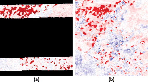
The method was run on all Landsat acquisitions from 1984 to 2014 for path 166, rows 066–067 and PALSAR acquisitions in fine-beam dual polarization from 2007–2010. For years with few satellite observations, Kalman filtering reduced large fluctuations from year to year (Figure 10). The inclusion of PALSAR data increased the estimated vegetation height for the 4 years with PALSAR data, 2007–2010. For both 2012 and 2014, when comparing the satellite estimates with the ALS nDSM, the deviation of the mean is low for all three versions of the method (Table 8). For change mapping, the method was able to capture most of the events of total biomass loss (Figure 11).

Table 8. Average vegetation height estimates for Liwale. Landsat data includes all Landsat-4, 5, 7 and 8 data (Landsat 7 SLC-off data is also included).

Satellite estimate	ALS data	# valid pixels	Satellite mean	ALS nDSM mean	Deviation of mean	R^2	RMSE	RMSE %
Landsat 7, 2012	2012	4,553,483	5.344 m	5.211 m	0.133 m	0.46	2.91 m	55.8
Landsat Kalman (1984) 2012	2012	4,586,329	5.332 m	5.203 m	0.119 m	0.51	2.81 m	54.0
Landsat + PALSAR, Kalman (1984) 2012	2012	4,586,309	5.327 m	5.203 m	0.123 m	0.53	2.74 m	52.7
Landsat 7 + 8, 2014	2014	4,636,822	5.309 m	5.234 m	0.086 m	0.51	3.03 m	58.0
Landsat Kalman (1984) 2014	2014	4,642,954	5.305 m	5.221 m	0.083 m	0.54	2.98 m	57.0
Landsat + PALSAR, Kalman (1984) 2014	2014	4,639,257	5.305 m	5.219 m	0.085 m	0.55	2.97 m	56.9

Figure 10. Estimated mean vegetation height for ALS area in Liwale.

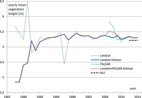
Figure 11. Change maps for a 7 km × 7 km area in Liwale. Red = reduction in vegetation height, blue = increase in vegetation height, white = unchanged. (a) ALS 2012–2014, up to 13.7 m reduced average height (darkest red) was measured within 30 m × 30 m pixels. The largest increase was 2.7 m (darkest blue). Black is no data. (b) Difference for 2012–2014 estimated from Kalman filtered multi-sensor time series, differences range from −8.6 to 5.2.

For the Amani area (Figure 4), which is a montane tropical forest with some trees taller than 50 m, the proposed method performs less well. PALSAR data could not be used for vegetation height estimation due to the steep topography. Therefore, only Landsat data were used: path 166, row 064 from 1984–2012. On average, for Landsat 2012 data, the method underestimated the mean vegetation height by 6.6 m (Table 9). Kalman filtering did not improve the bias, and the variance also remained high. However, Kalman filtering was able to provide estimates for 6814 pixels that lacked 2012 Landsat-7 coverage (Figure 12(a,b); Table 9). From the difference image (Figure 12(d)), we observe that the method overestimated the vegetation height in areas with low vegetation. For areas with high vegetation, the method underestimated the average vegetation height by up to 40 m. This is likely a saturation effect.

Table 9. Average vegetation height estimates for Amani.

Satellite estimate	ALS data	# valid pixels	Satellite mean	ALS nDSM mean	Deviation of mean	R^2	RMSE	RMSE %
Landsat 7, 2012	2012	129,975	12.26 m	18.91 m	6.647 m	0.29	13.43 m	71.0
Kalman filtered Landsat (1984) 2012	2012	136,789	12.15 m	19.07 m	6.922 m	0.34	13.57 m	71.2

Figure 12. Result of using the method on the Amani area. Grey values are scaled from 0 m (black) to 20 m (white), except for the difference image (d), which is scaled from −20 m (black) to 20 m (white). Areas outside of ALS coverage are set to 0 m. (a) Estimated vegetation height for 2012 from Landsat-7. Actual values range from 0 to 24 m. (b) Estimated vegetation height for 2012 from Landsat time series 1984–2012 with Kalman filtering. Actual values: 0–20 m. (c) ALS nDSM, actual values: 0–60 m. (d) Difference of estimates from Landsat with Kalman filtering and ALS, i.e. (b) minus (c). Actual values: −40 m to +25 m.

Discussion

The results of average vegetation height estimation show that it is possible to extract height information from Landsat images of forested areas provided the forest is not too dense. By using time series instead of individual images, the variance is reduced substantially. By adding PALSAR data to the time series, the variance might be further reduced.

For change detection, the results are less convincing. Areas with total loss of biomass were detected, but gradual changes are not captured well. The difficulties are due to the variation of the yearly height estimates from satellite. This variation is often larger than the actual change in vegetation height as measured by the ALS data.

The performance of the proposed method in terms of root means square error (Tables 8 and 9) is not convincing compared to existing methods (Table 1). However, most of these studies are on forests only, while our method has been applied on all land cover types, including agricultural fields and mixes of agriculture and tree vegetation.

We have based our study on a simple, linear regression between one vegetation index (SLAVI) derived from three satellite bands, and mean vegetation height. A regression on multiple vegetation indexes could be used with the goal to reduce the variance.

The regression between PALSAR mean backscatter and ALS (Figure 9) seem to deviate systematically from the fitted exponential curve, in that high vegetation values >17 m are underestimated while medium vegetation values 3–12 m are underestimated. Thus, a different parametric nonlinear function may produce better results.

On the other hand, a potential problem with the regression between PALSAR and ALS is that the PALSAR data are from 2007 to 2010 while the ALS data are from 2012. Thus, vegetation height changes between the PALSAR and ALS acquisitions are ignored. These changes may be a mix of height increase due to growth and decrease due to felling of individual trees and clear cuts. If we assume that high trees are more likely to be felled than small trees, while average height growth is more likely to occur in areas with low average vegetation height, then the systematic deviations observed in Figure 9 may be explained by the time difference of acquisitions.

Another way of reducing the variance is through more averaging, in time and/or space. Given the low number of acquisitions per year in 1984–1990, one may use the estimate for 1990 after Kalman filtering as the first year in the time series. For the purpose of reporting of carbon stocks, Tanzania needs to provide one single number every second year for the entire country. Since 90% of Tanzania is Miombo woodlands, on may use a regression between biomass and average vegetation height developed for Miombo woodlands. For each reporting year, one may run the processing chain on all the 48 path/row pairs that are needed to Cover Tanzania, mask areas outside of Tanzania, and produce one estimate for each path/row and then aggregate again to produce one single estimate for the entire country.

One strategy to obtain more optical observations from the past than may be provided by Landsat could be to include daily acquisitions at a coarser resolution, e.g. Modis (250 m–1 km resolution), VIIRS (375–750 m) or Sentinel-3 SLSTR (500–1000 m) and OLCI (300 m). It is straightforward to modify the Kalman filtering step to include more sensors. However, all images must be resampled to the same resolution.

To improve the accuracy of the method for present and future mean vegetation estimates, it seems obvious to include Sentinel-2 data, with 10 and 20 m pixel spacing instead of 30 m, and more frequent revisit. Another problem that Sentinel-2 may help to solve is that two 30 m × 30 m Landsat pixels with the same average height may have different spatial distributions of vegetation height. An area with 50% canopy cover of 20 m tall trees may have a different spectral and temporal signature than an area with 100% canopy cover and 10 m tall trees. By dividing each Landsat pixel into 3 × 3 Sentinel-2 pixels, these differences may become apparent, unless the 20 m high tree canopies that occupy 50% of one Landsat pixel are homogeneously distributed over the 3 × 3 Sentinel-2 pixels.

The method is developed for open forests and woodland landscapes, with gradual changes in tree crown cover. The method was calibrated with ALS data from Liwale, since this landscape is representative for the majority of forests and woodland landscapes in Tanzania. The method saturates at around 10 m average vegetation height. For tropical rain forests, like in Amani, large areas had too low estimates. However, the method may still work for the detection of logging, of which many may be illegal conducts when it takes place in rain forests in Tanzania.

Accurate estimation of vegetation height and biomass for all of Tanzania by ALS is not considered as a realistic alternative, given the high acquisition cost. Forest change detection is also possible with TerraSAR Tandem-X, but again the cost is prohibitive at the moment. Given the free access to optical satellite data at various resolutions, further research into automatic methods for the extraction of essential forest variables seems to be a viable alternative.

Conclusions

To conclude, we have demonstrated that estimation of mean vegetation height is possible from dense time series of optical and SAR satellite data. However, better accuracy in the height estimates is desired. With better resolution and higher acquisition frequency, Sentinel-2 may provide exactly that. We recommend further studies on applying the developed method on Sentinel-2 data.

Geolocation information

Liwale study area: S9°54ʹ, E37°38ʹ; Amani study area: S5°08ʹ, E38°37ʹ.

Acknowledgements

We thank the other project partners for fruitful collaboration. In addition to the authors’ institutions, the project partners include: Sokoine University of Agriculture (SUA), Morogoro, Tanzania; University of Dar Es Salaam, Institute of Resource Assessment (UDSM/IRA), Dar Es Salaam, Tanzania; Kongsberg Satellite Services (KSAT), Tromsø, Norway; Norwegian Institute of Bioeconomy Research (NIBIO), Ås, Norway; and The Arctic University of Norway (UiT), Tromsø, Norway. Special thanks go to Eliakimu Zahabu (SUA), Olipa Simon (UDSM), Harun Makandi (UDSM), Stian Normann Anfinsen (UiT), Svein Solberg (NIBIO), Annekatrien Debien (KSAT) and Line Steinbakk (KSAT). We thank Curtis Woodcock (Boston University), Richard Lukas (Aberystwyth University), Åke Rosenqvist and Leif Kastdalen for interesting discussions. We thank Evie Merethe Hagen and Per Erik Skrøvseth of the Norwegian Space Centre for facilitating the organization of the project. We also thank the anonymous reviewers for providing constructive feedback, improving the manuscript.

Disclosure statement

No potential conflict of interest was reported by the authors.

Additional information

Funding

This research was supported by the Norwegian Ministry of Foreign Affairs  (Utenriksdepartementet). PALSAR data were acquired from JAXA through the Global Forest Observation Initiative and the European Space Agency (ESA) category-1 proposal [Grant no. 27689].

References

- Aase, J.K., & Siddoway, F.H. (1981). Assessing winter wheat dry matter production via spectral reflectance measurements. Remote Sensing of Environment, 11, 267–277.
- Campbell, J.B. (2006). Introduction to remote sensing (4th ed.). Oxon, UK: Taylor and Francis.
- Cartus, O., Kellndorfer, J., Rombach, M., & Walker, W. (2012). Mapping canopy height and growing stock volume using airborne lidar, ALOS PALSAR and Landsat ETM+. Remote Sensing, 4, 3320–3345.
- Chopping, M., Nolin, A., Moisen, G.G., Martonchik, J.V., & Bull, M. (2009). Forest canopy height from the Multiangle Imaging SpectroRadiometer (MISR) assessed with high resolution discrete return lidar. Remote Sensing of Environment, 113, 2172–2185.
- Ene, L.T., Næsset, E., Gobakken, T., Bollandsås, O.M., Mauya, E.W., & Zahabu, E. (2017). Large-scale estimation of change in aboveground biomass in miombo woodlands using airborne laser scanning and national forest inventory data. Remote Sensing of Environment, 188, 106–117.
- Hansen, E.H., Gobakken, T., Bollandsås, O.M., Zahabu, E., & Næsset, E. (2015). Modeling aboveground biomass in dense tropical submontane rainforest using airborne laser scanner data. Remote Sensing, 7, 788–807.
- Hansen, M.C., & Loveland, T.R. (2012). A review of large area monitoring of land cover change using landsat data. Remote Sensing Of Environment, 122, 66–74. doi:10.1016/j.rse.2011.08.024
- Hansen, M.C., Potapov, P.V., Moore, R., Hancher, M., Turubanova, S.A., Tyukavina, A., … Townshend, J.R.G. (2013). High-resolution global maps of 21st-century forest cover change. Science, 342, 850–853.
- Helmer, E.H., Ruzycki, T.S., Wunderle, J.M., Jr., Vogesser, S., Ruefenacht, B., Kwit, C., … Ewert, D.N. (2010). Mapping tropical dry forest height, foliage height profiles and disturbance type and age with a time series of cloud-cleared Landsat and ALI image mosaics to characterize avian habitat. Remote Sensing of Environment, 114, 2457–2473.
- Hopkinson, C., Chasmer, L., Lim, K., Treitz, P., & Creed, I. (2006). Towards a universal lidar canopy height indicator. Canadian Journal of Remote Sensing, 32(2), 139–152.
- Hyyppä, J., Hyyppä, H., Inkinen, M., Engdahl, M., Linko, S., & Zhu, Y.-H. (2000). Accuracy comparison of various remote sensing data sources in the retrieval of forest stand attributes. Forest Ecology and Management, 128, 109–120.
- Ioki, K., Tsuyuki, S., Hirata, Y., Phua, M.-H., Wong, W.V.C., Ling, Z.-Y., … Takao., G. (2014). Estimationg above-ground biomass of tropical rainforest of different degradation levels in Northern Borneo using airborne LiDAR. Forest Ecology and Management, 328, 335–341.
- Jin, S., & Sader, S.A. (2005). Comparison of time series tasseled cap wetness and the normalizeddifference moisture index in detecting forest disturbances. Remote Sensing Of Environment, 94, 364 – 372. doi:10.1016/j.rse.2004.10.012
- Kalacska, M., Sanchez-Azofeifa, G.A., Rivard, B., Caelli, T., White, H.P., & Calvo-Alvarado, J.C. (2007). Ecological fingerprinting of ecosystem succession: Estimating secondary tropical dry forest structure and diversity using imaging spectroscopy. Remote Sensing of Environment, 108, 82–96.
- Kalman, R.E. (1960). A new approach to linear filtering and prediction problems. Journal of Basic Engineering, 82(1), 35–45.
- Kellndorfer, J., Walker, W., Pierce, L., Dobson, C., Fites, J.A., Hunsaker, C., … Clutter, M. (2004). Vegetation height estimation from Shuttle Radar Topography Mission and National Elevation Datasets. Remote Sensing of Environment, 93, 339–358.
- Kleynhans, W., Olivier, J.C., Wessels, K.J., Salmon, B.P., Van den Bergh, F., & Steenkamp, K. (2011). Detecting land cover change using an extended Kalman filter on MODIS NDVI time-series data. IEEE Geoscience and Remote Sensing Letters, 8(3), 507–511.
- Kugler, F., Schulze, D., Hajnsek, I., Pretzsch, H., & Papathanassiou, K.P. (2014). TanDEM-X pol-inSAR performance for forest height estimation. IEEE Transactions on Geoscience and Remote Sensing, 52(10), 6404–6422.
- Kwak, D.-A., Lee, W.-K., Lee, J.-H., Biging, G.S., & Gong, P. (2007). Detection of individual trees and estimation of tree height using LiDAR data. Journal of Forest Research, 12, 425–434.
- Larsen, Y., Engen, G., Lauknes, T.R., Malnes, E., & Høgda, K.A. (2005, November 28 – December 2). A generic differential interferometric SAR processing system, with applications to land subsidence and snow-water equivalent retrieval. Proceedings of the Fringe 2005 Workshop, Frascati, Italy.
- Lefsky, M.A. (2010). A global forest canopy height map from the moderate resolution imaging spectroradiometer and the geoscience laser altimeter system. Geophysical Research Letters, 37, L15401. doi:10.1029/2010GL043622
- Lefsky, M.A., Keller, M., Pang, Y., Camargo, P.B., & Hunter, M.O. (2007). Revised method for forest canopy height estimation from Geoscience Laser Altimeter System waveforms. Journal of Applied Remote Sensing, 1, 013537.
- Lei, Y., & Siqueira, P. (2014). Estimation of forest height using spaceborne repeat-pass L-band InSAR correlation magnitude over the US state of Maine. Remote Sensing, 6, 10252–10285.
- Lymburner, L., Beggs, P.J., & Jacobson, C.R. (2000). Estimation of canopy-average surface-specific leaf area using Landsat TM data. Photogrammetric Engineering & Remote Sensing, 66(2), 183–191.
- Mauya, E.W., Ene, L.T., Bollandsås, O.M., Gobakken, T., Næsset, E., Malimbwi, R.E., & Zahabu, E. (2015). Modelling aboveground forest biomass using airborne laser scanner data in the miombo woodlands of Tanzania. Carbon Balance and Management, 10, paper no. 28. doi:10.1186/s13021-015-0037-2
- Mitchard, E., Saatchi, S.S., Woodhouse, I., Nangendo, G., Ribeiro, N., Williams, M., … Meir, P. (2009). Using satellite radar backscatter to predict aboveground woody biomass: A consistent relationship across four different African landscapes. Geophysical Research Letters, 36, L23401.
- Næsset, E. (1997). Determination of mean tree height of forest stands using airborne laser scanner data. ISPRS Journal of Photogrammetry & Remote Sensing, 52, 49–56.
- Salberg, A.B., & Trier, Ø.D. (2011, July 24–29). Temporal analysis of forest cover using hidden Markov models. In Proceedings of the 2011 IEEE Geoscience and Remote Sensing Symposium (pp. 2322–2325). Vancouver, Canada. doi:10.1109/IGARSS.2011.6049674
- Salberg, A.B., & Trier, Ø.D. (2012, July 22–27). Temporal analysis of multisensor data for forest change detection using hidden Markov models. In Proceedings of the 2012 IEEE Geoscience and Remote Sensing Symposium (pp. 6749–6752). Munich, Germany. doi:10.1109/IGARSS.2012.6352556
- Sexton, J.O., Bax, T., Siqueira, P., Swenson, J.J., & Hensley, S. (2009). A comparison of lidar, radar, and field measurements of canopy height in pine and hardwood forests of southeastern North America. Forest Ecology and Management, 257, 1136–1147.
- Skidmore, A.K., Pettorelli, N., Coops, N.C., Geller, G.N., Hansen, M., Lucas, R., … Wegmann, M. (2015). Agree on biodiversity metrics to track from space. Science, 523, 403–405.
- Townshend, J.R.G., Goff, T.E., & Tucker, C.J. (1985). Multitemporal dimensionality of images of normalized difference vegetation index at continental scales. IEEE Transactions on Geoscience and Remote Sensing, 23(6), 888–895.
- Véga, C., & St-Onge, B. (2008). Height growth reconstruction of a boreal forest canopy over a period of 58 years using a combination of photogrammetric and lidar models. Remote Sensing of Environment, 112, 1784–1794.
- Wilkes, P., Jones, S.D., Suarez, L., Mellor, A., Woodgate, W., Soto-Berelov, M., … Skidmore, A. (2015). Mapping forest canopy height across large areas by upscaling ALS estimates with freely available satellite data. Remote Sensing, 7, 12563–12587.
- Wolter, P.T., Townsend, P.A., & Sturtevant, B.R. (2009). Estimation of forest structural parameters using 5 and 10 meter SPOT-5 satellite data. Remote Sensing of Environment, 113, 2019–2036.
- Zhang, G., Ganguly, S., Nemani, R.R., White, M.A., Milesi, C., Hashimoto, H., … Myneni, R.B. (2014). Estimation of forest aboveground biomass in California using canopy height and leaf area index estimated from satellite data. Remote Sensing of Environment, 151, 44–56.
- Zhu, Z., Wang, S., & Woodcock, C.E. (2015). Improvement and expansion of the Fmask algorithm: Cloud, cloud shadow, and snow detection for Landsats 4–7, 8, and Sentinel 2 images. Remote Sensing of Environment, 159, 269–277.
- Zhu, Z., Woodcock, C.E., & Olofsson, P. (2012). Continuous monitoring of forest disturbance using all available Landsat imagery. Remote Sensing of Environment, 122, 75–91.