A novel model of estimating sea state bias based on multi-layer neural network and multi-source altimeter data

ABSTRACT

In this article, we propose a novel model for estimating sea state bias (SSB) based on multi-layer neural network and multi-source altimeter data from the Topex/Poseidon (T/P), Jason-2, and Jason-3 altimeters. Significant wave height (SWH), wind speed (U) and backscatter coefficient (σ₀) are considered as the inputs of the multi-layer neural network, while the corresponding SSB as outputs. The neural network has four layers, with structure 3-3-6-1. Data from three seasons are employed for the neural network training, and the trained model is applied for the SSB estimation on the HY-2 altimeter data. To show the effectiveness of the adopted model, the correlations between SSB and SWH, U and σ₀ are analyzed. Moreover, the explained variance and residual error are compared with a conventional parametric model for SSB estimation. The results demonstrate that multi-layer neural network trained on multi-source altimeter data performs superior to the conventional SSB estimation model.

KEYWORDS:

• Sea state bias
• radar altimeter
• neural network

Introduction

In general, radar altimeters can directly measure multiple types of data, such as global sea surface height (SSH), significant wave height (SWH) and wind speed (U) (Gaspar et al., 2002). However, height measurement usually contains errors, which may be resulted from the orbit error, sea state bias (SSB) (Reale, Dentale, & Carratelli, 2014), ionosphere error and/or dry-wet troposphere error (Labroue et al., 2004). In recent years, with the development of precise orbiting technology, SSB surpasses the orbit error and becomes the most important part of the height measurement errors. Therefore, accurate estimation of SSB can greatly improve the accuracy of height measurements obtained using a radar altimeter (Miao et al., 2016).

In order to estimate SSB, one may use theoretical models or empirical models. However, theoretical models are essentially impractical, as it is very difficult to obtain a suitable function and necessary parameters. Alternatively, empirical models are widely used. Commonly used empirical models belong to either parametric models, nonparametric models or numerical model (Pugliese et al., 2007; Wang et al., 2014). Based on the Topex/Poseidon (T/P) radar altimeter data, Gasper et al. proposed a parametric model for estimating SSB that possessed simple principles, intuitive modeling and excellent extensibility (Gaspar et al., 1994). However, as this method is not a real least square fitting for SSB, there is deviation in the model coefficient (Zhang et al., 2016). Based on a T/P radar altimeter cross point data set, Gasper et al. introduced a nonparametric model for SSB estimation (Gaspar & Florens., 1998). Their nonparametric model is based on a kernel smoothing statistical technique. However, the modeling process is complex, requiring a large amount of computing power, and results in low efficiency and inferior extensibility. In addition, Vandemark et al. performed collinear processing on data from a T/P radar altimeter based on a reference trajectory, which was able to estimate SSB directly (Vabdemark et al., 2002). This direct estimation model is based on collinear data acquired over numerous cycles. Due to the large amount of data used in its calculations, its results are highly accurate. However, similar to a nonparametric model, bilinear interpolation is needed, which constrains the extensibility of the model.

This article aims to investigate a neural network model to SSB estimation based on radar altimeter data. McCleland and Rumelhart proposed a parallel distributed processing network, which led to research on neural network models (Karayiannis & Anastasios, 2010). The most influential of these models is the back-propagation (BP) algorithm proposed by David Rumelhart and James McCleland (Schmidhuber, 2015). This deep learning network model has large-scale parallel data processing capabilities; distributed storage and excellent fault tolerance, adaptability and self-organization (Odom & Sharda, 2012).

In this article, based on the geo-physical data records (GDR) from the T/P, Jason-2, and Jason-3 radar altimeters, data from 6 cycles during different seasons (February, June and October) are combined as a training set. The SWH, wind speed (U) and backscatter coefficient (σ₀) are used as input features to train a neural network model that has two hidden layers, while the actual SSB values are adopted as the expected output. The GDR data from cycles acquired from three radar altimeters during different seasons are used as a validation set to verify the effectiveness of the model. The derived neural network model is then applied to an HY-2 radar altimeter, and the results are better than the conventional parameter model. Here, for the training, validation and test of the proposed model, the Ku-band data in the GDR date set are used. As a result, we establish a neural network model to solve the problem of accurately estimating SSB, which can provide a new method for the further study of ocean phenomenon using radar altimeter data.

Model construction and testing

Data set

In this article, 6 cycles of the GDR data (3,190,448 groups) from the T/P, Jason-2 and Jason-3 radar altimeters in February, June and October between 2005 and 2016 are combined as a training set. Meanwhile, 3 cycles of the GDR data (1,347,033 groups) are used as validation data. Table 1 shows the details of the used data. According to the requirements on the quality of the radar altimeter data, along with SSB, error correction items such as instrument errors, dry and wet troposphere delays, ionosphere delays and inverse atmospheric pressure, high-frequency oscillations, tides, pole tides, solid earth tides and load tides are included in the altimeter height measurement data (Chambers et al., 2003). Abnormal data (SSH > 100 m or SSH < −130 m, SWH < 0 m or SWH > 11 m, U < 0 m/s or U > 21 m/s, σ₀ < 7 dB or σ₀ > 30 dB, and SSB >0 m or SSB < −0.5 m) are removed, and the data set is normalized (Gommenginger et al., 2003). SWH, U and σ₀ in GDR are used as model inputs, while SSB in GDR is used as the expected model output to train the neural network. Note that the SSB estimations in GDR of the T/P, Jason-2 and Jason-3 radar altimeters are all based on a nonparametric model with SWH and U as inputs (Gasper et al., 2002; Miao et al., 2016).

Table 1. The details of the used data set (cycles) .

	T/P (2005)		Jason-2 (2013 & 2016)		Jason-3 (2016)
	Training	Test	Training	Test	Training	Test
February	C457	C421			C001
June	C469		C293			C012
October			C305	C195	C025

Model construction

Traditional parametric or nonparametric models for SSB estimation usually use two features, SWH and U, as model inputs. However, SSB is essentially related to SWH, wind speed U and backscatter coefficient σ₀. Hence, in this work, we also consider the backscatter coefficient σ₀. For more details, the backscatter coefficient σ₀ can be directly measured by the radar altimeters. Although the models for computing the wind speed U generally take account of the backscatter coefficient σ₀, they use other parameters as well. Moreover, there are many models for computing the wind speed U, and these models may deliver different results on the computing of U. Hence, the backscatter coefficient σ₀ can provide important information about SSB, which SWH and U may not include. Motivated by the development of multi-layer neural networks in recent years, we attempt to train a neural network for the SSB estimation to obtain an effective model and accurate results.

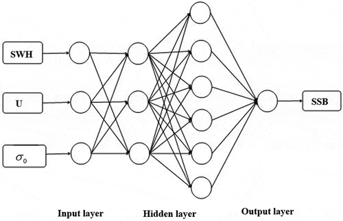
The architecture of the used network model has four layers, as shown in Figure 1. It is based on the BP algorithm (Byvatov et al., 2003). The three nodes in the input layer correspond to the features SWH, U and σ₀; only one node in the output layer corresponds to the estimated SSB value. Considering the complexity of the SSB estimation problem, two hidden layers are adopted in our model. Determining the number of hidden layer nodes is a complex problem for which there is no satisfactory analytical theorem (Lecun, Bengio, & Hinton, 2015). Generally, the number of nodes in the hidden layer is determined by function complexity: too many nodes may result in an excessively long network learning period, and too few nodes may result in low fault tolerance and inferior identification of unlearned samples (Ding et al., 2010). Based on previous experience, in this work, hidden layer node selection is based on the following reference formula:

(1)

Figure 1. Structure of the neural network model.

where n is the number of nodes in the input layer (n = 3) and q is the number of nodes in the output layer (q = 1); is a constant number (Bengio, 2013). After some empirical test, we found that, when a = 1, m = 3 for the first hidden layer and a = 4, m = 6 for the second hidden layer, the network could perform well for the SSB estimation task. Therefore, a network with structure 3-3-6-1 was used. The parameters for this neural network model were set as follows: the number of cyclic tests is res = 3; the number of iterations is , and the learning rate is (Ding et al., 2010). In addition, a nonlinear Tan-Sigmoid transmission function from the input layer to the hidden layer is used (Guo et al., 2011):

(2)

For the transmission function from the hidden layer to the output layer, we used the pure-linearity expression as follows (Ren, Yan, & Wang, 2007):

(3)

where k is a non-zero real number and b is the bias term.

Model evaluation

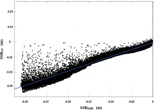
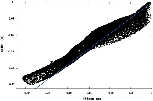
The effectiveness of the model is evaluated via the correlation coefficient (R²) and the standard deviation (S) of the model output SSB_NN (SSB of neural network) versus SSB_GDR (SSB of GDR) from the test set. When R² is closer to 1, SSB_NN and SSB_GDR are more highly correlated, and the model is more effective. A scatter diagram with a fitted regression line for these two values is shown in Figure 2. Meanwhile, smaller S values imply smaller differences. The results obtained on validation set are R² = 0.988 and S = 1.55 cm.

Figure 2. Scatter diagram with linear regression lines of SSB_NN and SSB_GDR.

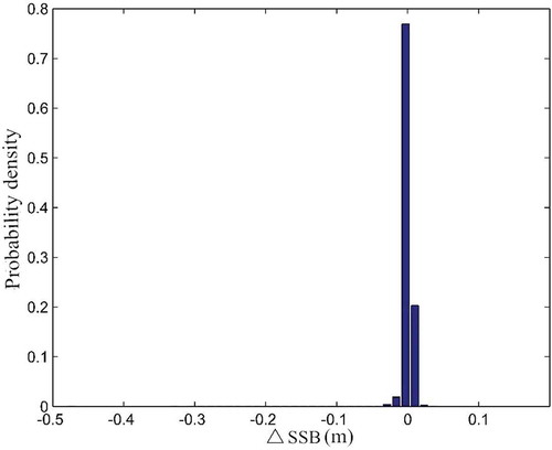
The density distribution of difference is shown in Figure 3. Model tests show that SSB_NN and SSB_GDR are highly consistent, implying that the network model is very effective.

Figure 3. Probability density distribution for ∆SSB.

Model application and discussion

The developed neural network model is applied to data from the 70^th and 71^st cycles (798,726 groups) of the HY-2 radar altimeter. It is because that these two cycles of data have been processed by the National Satellite Ocean Application Service of China, and their quality is relatively high. HY-2 SSB estimation has been performed based on a conventional parametric model. This parametric model is a biquadratic multi-variable Taylor polynomial function about SSB, which takes SWH and U as inputs. The parameters in this polynomial function are learned using regression method based on the least square estimation. For the HY-2 radar altimeter, a model including four parameters are applied (Li et al., 2013; Wang et al., 2014). To further verify the effectiveness of the neural network model, the following analyses are conducted: analysis of the correlation of SSB and SWH, U and σ₀; difference analysis; analysis of explained variance and residual error for results from the neural network model versus results from a conventional parametric model for GDR from an HY-2 altimeter.

Comparison between the NN and parametric models

The SSB results from the neural network model were compared with the SSB results from a conventional parametric model based on GDR from an HY-2 radar altimeter. A density distribution of the differences between the two () is shown in Figure 4, and a scatter diagram with a linear regression line is shown in Figure 5.

Figure 4. Probability density distribution for ∆SSB.

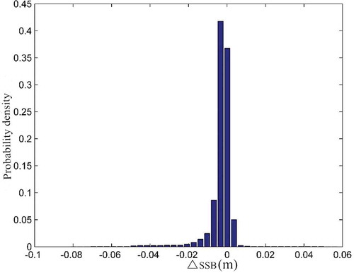
Figure 5. Scatter diagram with a linear regression lines for SSB_NN and SSB_GDR.

The standard deviation (S) for the two models is 1.80 cm; the average absolute SSB for the neural network model is 7.85 cm and the average absolute SSB for the conventional parametric model is 8.15 cm. Figure 4 shows that the majority of the differences are concentrated in the range from −1 to 0.5 cm, accounting for 95.26% of the overall data.

Based on Figure 5, the results from the neural network model and the results from the conventional parametric model are positively linearly correlated. When the absolute SSB is less than 15 cm, the absolute value from the neural network model is usually larger than the absolute SSB from the conventional parametric model. Furthermore, when the absolute SSB exceeds 15 cm, the absolute SSB from the neural network model is usually smaller than the absolute SSB from the conventional parametric model.

Correlation coefficient (R²) of SSB with SWH, U and σ₀

As the neural network model is based on the correlation of SSB with SWH, U and σ₀, the correlation analyses for SSB with SWH, U and σ₀ are performed separately. A higher correlation coefficient means that the residual error is smaller and that the model is more effective.

The correlation coefficients of SSB_NN with SWH, U and σ₀ from the neural network model are compared with correlation coefficients of SSB_GDR with SWH, U and σ₀ from the conventional parametric model. The values of the correlation coefficients (R²) are listed in Table 2, and the scatter diagrams with linear regression lines are shown in Figure 6–11.

Table 2. Correlation coefficients (R²) of SSB with SWH, U and σ_0.

	R^2
	SWH-SSB	U-SSB	σ0-SSB
Neural network model	0.95	0.49	0.67
Conventional parametric model	0.91	0.43	0.27

Figure 6. Scatter diagram with linear regression line for SSB_NN and SWH.

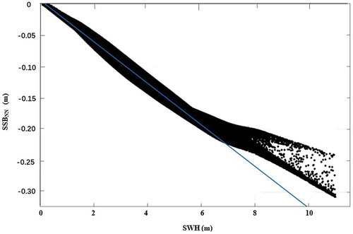
Figure 7. Scatter diagram with linear regression line for SSB_GDR and SWH.

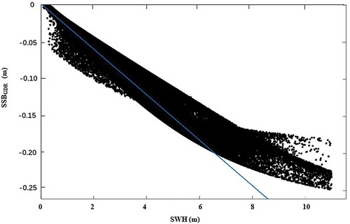
Figure 8. Scatter diagram with linear regression line for SSB_NN and U.

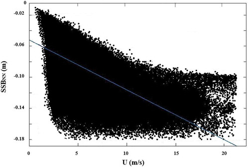
Figure 9. Scatter diagram with linear regression line for SSB_GDR and U.

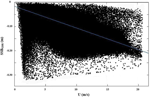
Figure 10. Scatter diagram with linear regression line for SSB_NN and σ_0.

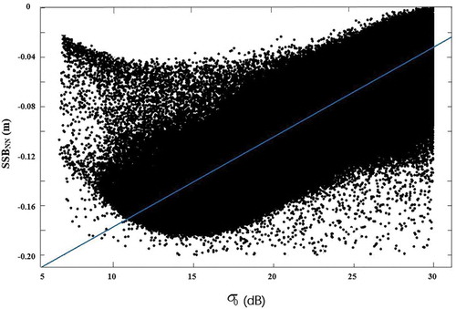
Figure 11. Scatter diagram with linear regression line for SSB_GDR and σ_0.

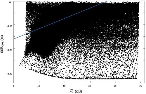
Table 1 and Figures 6–11 show that the SSB in the neural network model is more highly correlated with SWH, U and σ0 than the SSB in the conventional parametric model. Thus, the neural network model is more accurate and effective.

Explained variance (D)

Explained variance is the variance in the SSH deviation △SSH_i′ at a cross point without SSB correction minus the variance in the SSH deviation △SSH_i′–△SSB_i at a cross point with SSB correction. The explained variance is used to evaluate the effectiveness of the SSB model, where larger values mean that the model is more effective (Labroue et al., 2006).

The data at the cross points in the 70^th and 71^st cycles of an HY-2 radar altimeter (2997 groups) are extracted. The ascending and descending trajectory SSH values at the cross points are corrected via the SSB results from the neural network model and the parametric model. The explained variance in the neural network model is D_NN = 31.37 cm²; the explained variance in the parametric model is D_GDR = 30.69 cm². Thus, the neural network model is more effective than the conventional parametric model.

Residual error analysis

Based on the data at the cross points in the 70^th and 71^st cycles of an HY-2 radar altimeter, the correlation analysis for the residual error versus the SWH, wind speed and backscatter coefficient is performed for the results from the two models. The residual error calculation is based on Equation (4).

(4)

Subscript 1 denotes an ascending trajectory at the cross point, and subscript 2 denotes a descending trajectory at the cross point. The residual error is the SSH deviation at the cross point after SSB correction, and the SWH deviation, U deviation and σ₀ deviation at the cross point are divided into segments of (0.5 m, 0.5 m/s, 0.5 dB) (Tran et al., 2010). The average in each segment is calculated to analyze the correlation of the average residual error with △SWH, △U and △σ₀ in each segment. When the correlation is lower, the absolute average of for each segment is smaller, and the standard deviation S is smaller, indicating that the model is more effective (Li et al, 2013). The calculation results are listed in Table 3, and the residual error distributions are shown in Figure 12–17.

Table 3. Results and verification for a multi-layer neural network model and a GDR-based parametric model.

	-ΔSWH		-ΔU		-Δσ0
	Mean	Std	Mean	Std	Mean	Std
	(cm)	(cm)	(cm)	(cm)	(cm)	(cm)
Neural network model	0.55	2.98	0.41	1.72	0.45	3.79
Conventional parametric model	1.59	7.56	1.31	2.87	1.30	7.55

Figure 12. versus ∆SWH in the neural network model.

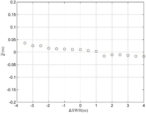
Figure 13. versus ∆SWH in the conventional parametric model.

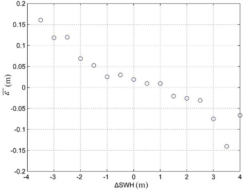
Figure 14. versus ∆U in the neural network model.

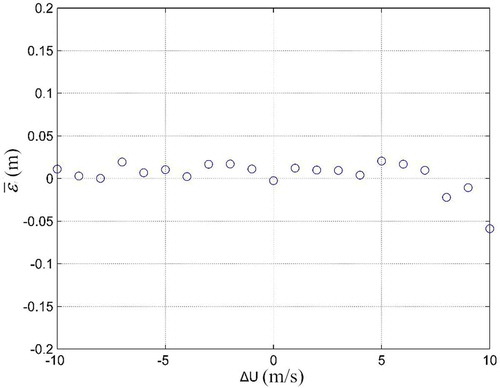
Figure 15. versus ∆U in the conventional parametric model.

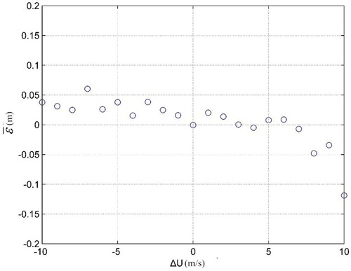
Figure 16. versus △σ₀ in the neural network model.

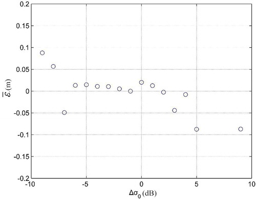
Figure 17. versus △σ₀ in the conventional parametric model.

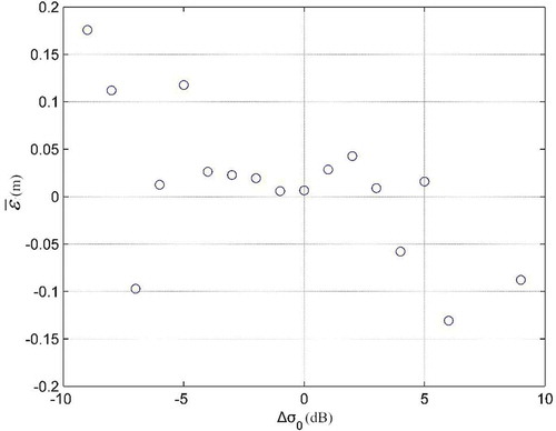
These results show that in the conventional parametric model, compared to the variations in ∆SWH, ∆U and ∆σ₀, the overall variation in is significant. In contrast, obtained via the neural network model is closer to 0, and its fluctuation is less severe. Thus, the neural network model is more effective for SSB estimation.

Conclusion

In this article, based on data from the T/P, Jason-2 and Jason-3 radar altimeters, data sets from six cycles acquired during different seasons are used to train a multi-layer neural network model. After validation, the model is applied to the 70^th and 71^st cycles of an HY-2 radar altimeter. The results from the neural network model and from a conventional parametric model are compared, showing that the root-mean-square deviation for the two models is 1.80 cm. In the neural network model, the correlation coefficients of SSB with SWH, U and σ₀ are 0.95, 0.49 and 0.67, respectively. In the conventional parametric model, the correlation coefficients of SSB with SWH, U and σ₀ are 0.91, 0.43 and 0.27, respectively. The explained variances of the data set at the cross points in the 70^th and 71^st cycles of HY-2 for the two models are 31.37 and 30.69 cm², respectively. The statistics and distribution of the model residual errors show that the neural network model is significantly superior to the conventional parametric model.

Disclosure statement

No potential conflict of interest was reported by the authors.

Additional information

Funding

This work was supported by the National Key R&D Program of China under Grant 2016YFC1401004, National Natural Science Foundation of China under Grant 41176157, National Natural Science Foundation of China under Grant 41406197 and Science and Technology Program of Qingdao, China under Grant 17-3-3-20-nsh.

References

- Bengio, Y. (2013). Deep learning of representations: looking forward.Proceedings of the First international conference on Statistical Language and Speech Processing .7978, 1–37.
- Byvatov, E., Fechner, U., Sadowski, J., & Schneider, G. (2003). Comparison of support vector machine and artificial neural network systems for drug/nondrug classification. Journal of Chemical Information and Computer Sciences, 43, 1882–1889.
- Chambers, D.P., Hayes, S.A., Ries, J.C., Urban T.J. (2003). New TOPEX sea state bias models and their effect on global mean sea level. Journal of Geophysical Research Oceans, 108, C10.
- Ding, S., Jia, W., Su, C., & Chen, J. (2010). An improved BP neural network algorithm based on factor analysis. Journal of Convergence Information Technology, 5, 103–108.
- Gaspar, P., & Florens, J.P. (1998). Estimation of the sea state bias in radar altimeter measurements of sea level: Results from a new nonparametric method. Journal of Geophysical Research, 103, 15803–15814.
- Gaspar, P., Labroue, S., Ogor, F., Lafitte, G., Marchal, L., & Rafanel, M. (2002). Improving nonparametric estimates of the sea state bias in radar altimeter measurements of sea level. Journal of Atmospheric & Oceanic Technology., 19, 1690–1707.
- Gaspar, P., Ogor, F., Le Traon, P.-Y., & Zanife, O.-Z. (1994). Estimating the sea state bias of the TOPEX and POSEIDON altimeters from crossover differences. Journal of Geophysical Research, 99, 24981–24994.
- Gommenginger, C.P., Srokosz, M.A., Wolf, J., & Janssen, P.A.E.M. (2003). An investigation of altimeter sea state bias theories. Journal of Geophysical Research Oceans, 108, 3011.
- Guo, Z., Wu, J., Lu, H., & Wang, J. (2011). A case study on a hybrid wind speed forecasting method using BP neural network. Knowledge-Based Systems, 24, 1048–1056.
- Karayiannis, N.B., & Anastasios, N.V. (2010). Artificial neural networks. Springer International, 31, 709–724.
- Labroue, S., Gaspar, P., Dorandeu, J., & Femenias, P. (2006). Overview of the improvements made on the empirical determination of the sea state bias correction. American Journal of Agricultural Economics, 614, 77.
- Labroue, S., Gaspar, P., Dorandeu, J., Zanifé, O.Z., Mertz, F., Vincent, P., & Choquet, D. (2004). Nonparametric estimates of the sea state bias for the Jason-1 radar altimeter. Marine Geodesy, 27, 453–481.
- Lecun, Y., Bengio, Y., & Hinton, G. (2015). Deep learning. Nature, 521, 436–444.
- Li, S., Wang, Y., Miao, H.L., & Zhou, X. (2013). A parametric model of estimating sea state bias based on JASON-1 altimetry.Zhongguo Shiyou Daxue Xuebao, 37, 15–22.
- Miao, H.L., Zhang, G.S., Wang, G., Guo, Y.T., Jing, Y., & Zhang, J. (2016). HY-2 altimeter sea state bias of non-parametric estimation model. Remote Sensing Technology and Application, 31, 1031–1036.
- Odom, M.D., & Sharda, R. (2012). A neural network model for bankruptcy prediction. IJCNN International Joint Conference on Neural Network. 2, 163-168.
- Pugliese Carratelli, E., Dentale, F., & Reale, F. (2007). Reconstruction of sar wave image effects through pseudo random simulation. In Proceedings of the Envisat Symposium 2007. ESA SP-636.
- Reale, F., Dentale, F., & Carratelli, E.P. (2014). Numerical simulation of whitecaps and foam effects on satellite altimeter response. Remote Sensing, 6, 3681–3692.
- Ren, J., Yan, W., & Wang, Y. (2007). The satellite altimeter wind speed retrieval algorithm based on neural network. Journal of Marine Technology., 26, 47–50.
- Schmidhuber, J. (2015). Deep learning in neural networks: An overview. Neural Networks., 61, 85–117.
- Tran, N., Vandemark, D., Labroue, S., & Picot, N. (2010). Sea state bias in altimeter sea level estimates determined by combining wave model and satellite data. Journal of Geophysical Research Oceans.115, 1-7.
- Vabdemark, D., Tran, N., Beckley, B.D., Chapron, B., & Gaspar, P. (2002). Direct estimation of sea state impacts on radar altimeter sea level measurements. Geophysical Research Letters, 29, 48–52.
- Wang, G.Z., Miao, H.L., Wang, X., Wang, Y., & Zhang, J. (2014). Study on parametric model of sea state bias in altimete based on fusion dataset of collinear and crossover. Remote Sensing Technology and Application, 29, 176–180.
- Zhang, G.S., Miao, H.H., Wang, G., Guo, Y.T., Jing, Y., & Zhang, J. (2016). Study on different latitude interval parameter estimation of radar altimeter sea state bias. Remote Sensing Technology and Application, 31, 1054–1058-1082.