Integrating terrestrial and airborne laser scanning for the assessment of single-tree attributes in Mediterranean forest stands

ABSTRACT

The development of laser scanning technologies has gradually modified methods for forest mensuration and inventory. The main objective of this study is to assess the potential of integrating ALS and TLS data in a complex mixed Mediterranean forest for assessing a set of five single-tree attributes: tree position (TP), stem diameter at breast height (DBH), tree height (TH), crown base height (CBH) and crown projection area radii (CPAR). Four different point clouds were used: from ZEB1, a hand-held mobile laser scanner (HMLS), and from FARO® FOCUS 3D, a static terrestrial laser scanner (TLS), both alone or in combination with ALS. The precision of single-tree predictions, in terms of bias and root mean square error, was evaluated against data recorded manually in the field with traditional instruments. We found that: (i) TLS and HMLS have excellent comparable performances for the estimation of TP, DBH and CPAR; (ii) TH was correctly assessed by TLS, while the accuracy by HMLS was lower; (iii) CBH was the most difficult attribute to be reliably assessed and (iv) the integration with ALS increased the performance of the assessment of TH and CPAR with both HMLS and TLS.

KEYWORDS:

• Remote sensing
• proximal sensing
• LiDAR
• forest inventories
• forest structure
• precision forestry

Introduction

Over the last several decades, airborne laser scanning (ALS) demonstrated to be useful in providing accurate estimations of tree heights and forest attributes related to tree spatial arrangement (Hyyppä, Holopainen, & Olsson, 2012). However, ALS data alone may not completely capture the information on the vertical distribution of the canopy because of the attenuation of the laser impulses, particularly in complex multi-layered and dense forests (Lim, Treitz, Wulder, St-Onge, & Flood, 2003). ALS-based estimations rely on the acquisition of information in the field from a sample extracted from the investigated forest area, usually in circular plots selected in the framework of a statistical sampling design (Chirici, McRoberts, Fattorini, Mura, & Marchetti, 2016; Corona, 2016).

Conventional forest mensuration in sampling plots is based on tree measurements carried out by mechanical or optical instruments, such as callipers, hypsometers, compass and measuring tapes. The development of laser scanning technologies is gradually modifying methods for assessing forest attributes in the field (Holopainen et al., 2013; Kankare et al., 2015; Moskal & Zheng, 2011). These technologies can improve work efficiency in forest inventory, potentially replacing manually measured tree attributes with more automatic procedures (Henning & Radtke, 2006; Liang et al., 2016). Hence, static and mobile terrestrial laser scanners are acquiring increasing relevance in forestry (Liang et al., 2016). Forest stand structure, especially the vertical distribution of forest vegetation, can be detected with high detail by laser scanners, providing single-tree estimations better than those obtained by remote sensing or traditional field measurements (Loudermilk et al., 2009). Furthermore, TLS data can be used to assess single-tree attributes which can be hardly measured with other methods, such as tree architecture or detailed tree assortments (Dassot, Constant, & Fournier, 2011).

The use of TLS for forest and tree mensuration can be classified according to the requested level of complexity of the attributes to be produced (Liang et al., 2016): from basic attributes such as the stem diameter at breast height (DBH), tree height (TH), tree position (TP) and three-dimensional (3D) models of the main stem, up to the provisioning of additional structural parameters such as crown width, crown projection area, crown height, crown surface area, secondary branches and leaves.

Static TLS is suitable to measure millimetre-level information from a sample plot level to a single tree (Kankare et al., 2013, 2014; Liang, Hyyppä, Kaartinen, Holopainen, & Melkas, 2012; Liang, Kankare, Yu, Hyyppa, & Holopainen, 2014; Lindberg, Holmgren, Olofsson, & Olsson, 2012; Maas, Bienert, Scheller, & Keane, 2008). The penetration of the laser pulse through the canopy is one of the main cause of measurements uncertainties. For instance, tree height underestimation occurs when LiDAR (Light Detection and Ranging) point density in the upper canopy is reduced due to the occlusion caused by the lower portion of tree canopy and understory vegetation (Maas et al., 2008). TLS point density is in fact negatively correlated with tree height (Van Der Zande, Hoet, Jonckheere, Van Aardt, & Coppin, 2006). Furthermore, TLS accuracy is influenced by other factors such as tree distance from the scanner, number of scans and DBH extraction method (Liang et al., 2016; Srinivasan, Popescu, Eriksson, Sheridan, & Ku, 2015). The hardware costs are still rather high (albeit even more decreasing) and the mobility of instruments is relatively low.

The disadvantages of TLS are partially reduced by mobile laser scanning technology, which allows a significant increase in productivity (e.g. area covered per hour of survey) and thus in capability of collecting inventory data over large areas (Ryding, Williams, Smith, & Eichhorn, 2015). Distinctively, hand-held mobile laser scanner (HMLS) has lower hardware costs compared to TLS and, using simultaneous localization and mapping (SLAM) methods, the reliance on satellite positioning is no longer needed (Ryding et al., 2015). At the same time, HMLS is less precise providing less accurate estimation of tree position and structure, in particular for smaller trees, than TLS. However, when trees with DBH <10 cm are not considered, even better results by HMLS, at least in DBH estimations, can be achieved (Bauwens et al., 2016; Ryding et al., 2015).

The integration of TLS and HMLS scans with ALS provides a further possible solution to enhance characterization of forest stand overstory and understory. In this case, accurate tree heights are measured using ALS returns and the tree positions and structure mainly on the basis of TLS or HMLS returns, so that integrating terrestrial scans and ALS data results in an improvement of measurement accuracy.

Few studies have focused on the analysis of the benefits resulting from TLS and HMLS merging with ALS (e.g. Hauglin, Lien, Næsset, & Gobakken, 2014; Paris, Kelbe, Van Aardt, & Bruzzone, 2015; Yang, Zang, Dong, & Huang, 2015), and no studies were carried out under complex Mediterranean environments, at least to our knowledge. In this study, our main objective was to assess and compare the precision and accuracy of ZEB1 HMLS and FARO® FOCUS 3D TLS to measure single-tree attributes within a complex mixed Mediterranean forest. In particular, we considered the following attributes: TP, DBH, TH, crown base height (CBH) and the radii of the crown projection area (CPAR). Using conventional field survey as a benchmark, the main aim was to compare tree-level attributes obtained by the automatic elaboration of four different point clouds: (i) HMLS, (ii) TLS, (iii) integration of HMLS and ALS (HMLS_ALS) and (iv) integration of TLS and ALS (TLS_ALS). The accuracy of the estimates was evaluated on the basis of bias and root mean square error (RMSE) calculated comparing tree-level estimations with field reference data.

This research note is organized as follows. First, the study area, field reference data and HMLS TLS, and ALS data are presented. Then, a concise description of the approach applied to align the different point clouds and the automatic procedure to derive single-tree attributes are reported. Finally, the results are discussed to highlight pros and cons of mobile (HMLS) and static (TLS) laser scanning techniques, as well as their potential integration with ALS for single-tree attribute estimation.

Material

Study area and field reference data

The study area is located in a Mediterranean dense and multi-layered forest stand close to Firenze (Central Italy), dominated by coniferous (Cupressus sempervirens L. and Pinus pinaster Aiton) and evergreen broadleaves (Quercus ilex L.), that can be ascribed to the type 9.1 of the European Forest Types (Barbati, Marchetti, Chirici, & Corona, 2014; Giannetti et al., 2017).

The field data were acquired on 18 March 2016 within one circular plot having a radius of 13 m (531 m²). The latitude and longitude of the centre of the plot were recorded by a GNSS receiver Trimble Geo 7X (Raunheim, Germany), which lasted for approximately 1 h with a 2-s logging rate. The post-processed centre coordinates revealed standard deviations of 0.8, 0.6 and 1.8 cm, respectively, for x, y and z.

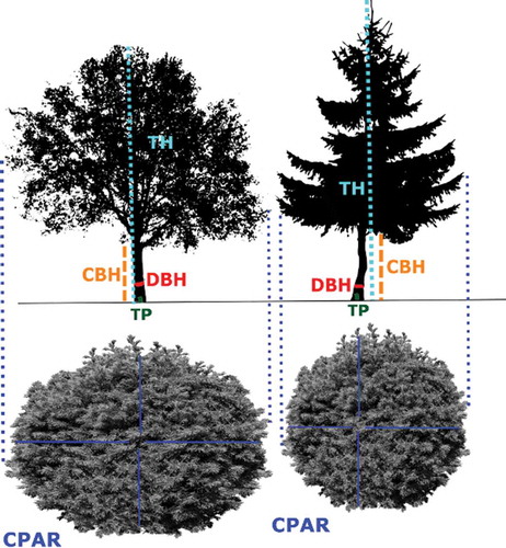
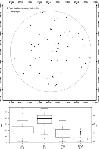
For all living and dead trees with DBH >2.5 cm, the following attributes were collected: horizontal distance and azimuth from the plot centre to compute TP, tree species, DBH, TH, and CBH. In addition, crown projection area (CPA) was calculated using the four crown radii (CPAR) measured in the field at each cardinal direction (north, east, south and west). DBH was measured with a calliper, TH, CBH and CPAR and horizontal distances were measured with a Vertex IV Hypsometer (Klockargatan, Sweden), while the azimuth was collected with a Suunto KB-14/360 R compass. A total of 56 stems (i.e. 52 living trees and 4 standing dead trees) and 224 CPAR were measured (Figure 1).

Figure 1. Graphical scheme of single-tree attributes measured in the field.

The measured stems had an average DBH of 20.8 cm (standard deviation (SD) of 9.6 cm), an average height of 12.5 m (SD of 3.92 m), an average CBH of 4.76 m (SD of 3.06 m) and an average CPAR of 1.66 m (SD of 1.30 m) (Figure 2).

Figure 2. Summary of the reference field data measured with traditional instruments. Above the single-tree position, below the boxplot of resulting values for DBH, TH, CBH, and CPAR.

These measures, collected by traditional instruments, are here assumed as error free and used as reference field data for evaluating the estimates produced on the basis of the different laser scans.

Laser scanner data collection and pre-processing

Hand-held mobile laser scanning

Like HMLS we used the ZEB1, which is a personal laser scanner instrument combined with an inertial measurement unit (IMU). The reported operative laser range outdoor is 15–20 m around the instrument (Bosse, Zlot, & Flick, 2012) with a scan ranging noise of ± 30 mm (GEOSLAM, 2016). Data acquisition is conducted by a person walking with the instrument through the plot (Bauwens et al., 2016; Ryding et al., 2015). Only one walking scan was needed to acquire the field plot. A complete description of the instrument can be found in Giannetti et al. (2017), Bauwens et al. (2016) and Ryding et al. (2015).

Data acquisition was carried out on 22 March 2016. Six spherical targets (each with a diameter of 14 cm) were fixed on the ground at different cardinal positions and at different distances from the centre to georeference the point cloud in post-processing (Figure 3). The spherical targets were measured using a GNSS receiver Trimble Geo 7X, which lasted for approximately 20 min with a 2-s logging rate. The post-processed spherical target coordinates revealed SDs of 0.7, 0.5 and 1.7 cm, respectively, for x, y and z. According to Bauwens et al. (2016), a walking fixed path was followed by the ZEB1 user to avoid shadow zones; the start and final points of the walking scan acquisition were coincident and fixed in the centre of the plot to ensure a close loop, as requested when the GEOSLAM algorithm is used.

Figure 3. The HMLS (ZEB1) walking scheme acquisition.

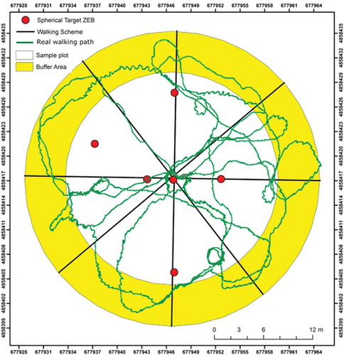
In the field, for the operator it was not easy to follow the desired theoretical path in the presence of obstacle on the ground. As a consequence, the real walking path resulted not coincident with the fixed one (Figure 3).

The raw ZEB1 data were processed with the in-house procedure GeoSLAM, which uses the SLAM algorithm to locate the scanner in an unknown environment position/location and to register the whole 3D point clouds using IMU data and feature detection algorithms (Bauwens et al., 2016). These algorithms permit us to build the 3D point cloud without the alignment of multiple scans. In fact these algorithms are able to built the whole 3D point cloud thanks to the trajectory calculated using the IMU data of the instrument and authomatically detection of equal features. More details on how this algorithm works can be found in the user’s manual of ZEB1 (GEOSLAM, 2016) and online at https://geoslam.com/slam/.

The 3D point cloud we obtained was rotated and translated using the six spherical targets from the local coordinate system to a geographic coordinate system (i.e. WGS84 UTM32N). The six spherical targets were automatically detected in the cloud using Cloud Compare software (France) (Compare Cloud, 2017) and with the align point pairs picking tools implemented in this software the reference coordinate system has been assigned. The final RMSE of roto-translation was 3.83 cm.

Static terrestrial laser scanning

Like TLS we used the FARO FOCUS 3D instrument that acquires data from eight fixed points through a scan angle of 360°. The instrument uses a phase-shift-based technology with a maximum range of 120 m. It is able to record and measure the x, y and z coordinates and the intensity of laser returns with a scan ranging noise of ± 1 mm (FARO, 2011). A complete description of the instrument can be found in Bauwens et al. (2016) and Ryding et al. (2015).

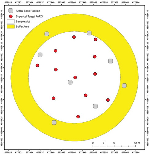
According to results reported by Trochta, Král, Janík and Adam (2013), several scans are needed in a forest field plot to acquire 50% of the DBH cross section and to detect 90% of the trees. Data acquisition was carried out on 25 March 2016. Given the complexity of the forest, eight static scans were acquired to avoid shadow zones. We used 12 spherical targets mounted on poles to co-register the different scans. One spherical target was fixed on the plot centre and the remaining were distributed within the plot to ensure the larger scans visibility; in order to obtain a good post-processing co-registration, scan positions were chosen to ensure as much as possible the higher inter-visibility of one scan to each other and the larger number of spherical targets (Figure 4).

Figure 4. TLS (FARO) scheme acquisition and the location of the 12 spherical targets used to align the scans.

The FARO scan system was set to obtain black-and-white scans that allow us to collect for each point the coordinates (i.e. x, y, z) and the intensity, with an intermediate resolution (i.e. the distance between two points in all directions at 10 m is equal to 9 mm).

The different scans were co-registered using Trimble RealWorks software (Raunheim, Germany) (Trimble, 2017) through the automatic detection of the spherical targets. All the spherical targets were recognized and the different scans were merged together in one-point cloud with an accuracy of ± 2 mm.

Airborne laser scanning

The ALS survey was carried out in May 2015 with a Eurocopter AS350 B3 (France) equipped with a LiDAR RIEGL LMS-Q680i (Horn, Austria) sensor. The flight height was 1100 m a.t.l. and the helicopter speed was 70 knots. The flight was planned to have an overlap between the strep of 30%. The LiDAR RIEGL LMS-Q680i sensor was set to acquire full-waveform LiDAR data that were in post-processing registered and discretized to a point density of 10 points m⁻² georeferenced in WGS84 UTM32N using the correction of the trajectories of the helicopter with the GNSS two base stations near the area of the Italtopos network and the IMU data collecting during the flight with a IMU of 400 Hz. The geographic accuracy of the acquisition was in sub-centimetres. Common procedures for pre-processing ALS data (e.g. outliers and noise cleaning, classification of ground/non-ground points and computation of height) were performed using LAStools software (Gilching, Germany). For more information on this ALS acquisition and the pre-processing techniques, please refer to Chirici et al. (2018).

Co-registration of point clouds

To allow the comparison of the two different point clouds (i.e. TLS and HMLS) and ease the analysis at single-tree level, the TLS point cloud was co-registered to the georeferenced HMLS cloud following the procedure described in Bauwens et al. (2016). A rough alignment in Cloud Compare (http://cloudcompare.org) software with the align function (Compare Cloud, 2017) was done using as corresponding points the trees in the plot identified by visual interpretation. The accuracy of the rough alignment calculated on the corresponding points was 5 cm. To obtain the best overall fit of the two point clouds and to improve the alignment accuracy, a hybrid multi-station adjustment (Trimble, 2017) was also carried out using a digital terrain model (DTM) extracted and automatically aligned from the point clouds themselves. The achieved accuracy was 2 cm.

In addition, the two point clouds (i.e. TLS and HMLS) were merged with ALS using the reference coordinate system (WGS84 UTM 32 N). The accuracy of the merging process was calculated on the basis of differences between terrain heights from the DTM based on ALS (i.e. derived by ground point) and the DTM obtained by TLS and HMLS. The TLS and HMLS DTMs that were calculated on the base of ground points classified with Computree (France) (http://computree.onf.fr) resample to a raster grid with a spatial resolution of 0.5 m. The RMSE between all the pixels revealed a mean difference of 2 and 3 cm for TLS and HMLS, respectively. As a result of this procedure, we obtained four georeferenced point clouds, namely TLS, HMLS, TLS_ALS and HMLS_ALS, which were used in the following analysis.

Methods

Extraction of single-tree attributes

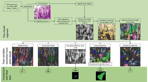
The Computree software (http://computree.onf.fr) was used to automatically extract the five considered single-tree attributes (TP, DBH, TH, CBH, CPAR) from the four point clouds. This approach allows the automatic extraction of all the attributes by the algorithms implemented in several tools. Simple trees tools (Hackenberg, Spiecker, Calders, Disney, & Raumonen, 2015) were used to segment the plot point clouds into single-tree point clouds, and to extract the single-tree attributes related to height (TH and CBH), DBH and TP. The ONF-ENSAM tools (Othmani, Piboule, Krebs, Stolz, & Voon, 2011) were used to determine the CPA for each single tree. The four radii (CPAR) of the CPA were derived from the crown projection area in a GIS environment. Figure 5 shows the workflow used to process the four point clouds.

Figure 5. Procedure used to automatically extract the single-tree attribute from the TLS (FARO) and HMLS (ZEB1) point clouds.

Accuracy assessment

For each considered single-tree attribute, we compared the estimation obtained by point clouds with the traditional manual field measures. To assess the accuracy of the tree-level estimations, we calculated the coefficient of determination (R²). A paired t-test was used (95% critical significant level, α=0.05) to test statistical differences. In addition, we calculated the RMSE and bias as follows:

where n is the number of trees measured in the field, is the true value of the attribute measured in the field and is the estimated value of the attribute for each ith tree. We used the Euclidean distance from the plot centre as and to calculate the RMSE and bias for TP.

Results

The automatic procedure allowed the segmentation of all the target trees measured in the field using HMLS, TLS, HMLS_ALS and TLS_ALS point clouds. The coefficient of determination (R² = .98 for x coordinate and R² = .99 for y coordinate) and t-test (p >.9) revealed a good fit between the tree position extracted from the four point clouds and the corresponding field reference measures (Figure 6). For TP, bias and RMSE were approximately 2.0 and 9.3 cm, respectively, independently of the cloud used (Table 1). A t-test confirmed that no significant differences (p >.90) exist among the different clouds.

Figure 6. Performance of tree position assessment on the basis of HMLS (ZEB1) and TLS (FARO) point clouds. Values in metres. The black line is the 1:1 line.

Table 1. Summary statistics of single-tree attributes detected by each point clouds. Superscript “a” indicate significant differences between the results obtained by the point cloud analysis and the measures in the field (t-test, p <.05).

Attributes	Point cloud	RMSE	Bias
Tree position (cm)	HMLS	9.31	2.06
	HMLSALS	9.31	2.06
	TLS	9.32	2.07
	TLSALS	9.32	2.07
Stem diameter at breast height (cm)	HMLS	1.28	−0.38
	HMLSALS	1.28	−0.38
	TLS	1.13	−0.41
	TLSALS	1.13	−0.41
Tree height (m)	HMLS	2.15	−4.61^a
	HMLSALS	0.94	−0.30
	TLS	0.88	−0.61
	TLSALS	0.43	−0.19
Crown base height (m)	HMLS	1.91	1.67 ^a
	HMLSALS	1.91	1.67 ^a
	TLS	1.95	1.82 ^a
	TLSALS	1.95	1.82 ^a
Crown projection area radii (m)	HMLS	0.59	0.25 ^a
	HMLSALS	0.44	0.20
	TLS	0.49	0.24
	TLSALS	0.24	0.18

For the DBH estimations, the coefficient of determination revealed a good fit between DBH estimated by HLMS (p >.90; R² = .99) and TLS (p >0.80; R² = .99) and the field reference measures (Figure 7). Comparable results in terms of bias and RMSE were observed between the two instruments. As for TP, the merging of ALS cloud did not increase the accuracy of DBH estimations. The results provided by TLS_ALS and HMLS_ALS were equal to those obtained by TLS and HMLS (R² = 1) (Table 1). However, using TLS and TLS_ALS clouds it was possible to detect 55 DBHs (DBH >2.5 cm) of the 56 trees measured in the field with conventional instruments while with HMLS and HMLS_ALS only 53 DBHs (DBH >5 cm) were detected.

Figure 7. Performance of DBH assessment on the basis of HMLS (ZEB1) and TLS (FARO) point clouds, both alone and integrated with ALS. Values in centimetres. The black line is the 1:1 line.

TH estimated by HMLS registered a large bias (Table 1 and Figure 8) and significant differences with reference field measures (p <.05 and R² = .94), while TLS produced more accurate results (p >.5; R² = .98) both in terms of bias and RMSE (Table 1 and Figure 8).

Figure 8. Performance of tree height assessment on the basis of HMLS (ZEB1) and TLS (FARO) point clouds, both alone and integrated with ALS. Values in metres. The black line is the 1:1 line.

RMSE of TH estimation was on average 17.2% (2.15 m) of the truth values when calculated on the basis of the HMLS cloud alone, and 7% (0.88 m) when based on the TLS cloud. As expected, the inclusion of the ALS cloud contributed in obtaining better results in the estimation of TH, especially for HMLS_ALS for which a consistent decrease of bias and RMSE (7.4% of the truth values) was observed. Concurrently, the coefficient of determination (R² = .97) and t-test (p >.7) revealed a good fit between TH estimated by HMLS_ALS and the field measures. The same positive effect by ALS integration was observed using TLS_ALS in terms of bias and RMSE (Table 1), which moved to 3.4% of the truth value (p >.8; R² = .99) (Figure 8).

We were able to estimate the CBH of all the segmented trees, both on the basis of HMLS and TLS clouds, but independently of the considered cloud or of the inclusion of ALS data, we registered always low accuracies, with R² being equal to .85, consistent bias and relatively high RMSE (Table1). The t-test between the CBH values estimated by clouds revealed a significant difference with the ones measured in the field (p <.05), with RMSE equal, on average, to 40% (1.91 m) and 41% (1.95 m) of the reference values for HMLS and TLS, respectively (Table 1). However, no significant differences were found (p >.9; R² = .99) between the results obtained by HMLS and TLS (Figure 9) with a constant underestimation especially for stems with larger CBH.

Figure 9. Performance of crown base height assessment on the basis of HMLS (ZEB1) and TLS (FARO) point clouds, both alone and integrated with ALS. Values in metres. The black line is the 1:1 line.

The CPAR estimation using HMLS and TLS alone showed significant differences with reference field measures (p <.05; HMLS: R² = .91; TLS: R² = .93), showing large bias with RMSE values equal, on average, to 36% (0.59 m) and 29% (0.88 m) of the reference values for HMLS and TLS, respectively (Figure 10). As reported for TH, the inclusion of the ALS cloud contributed in obtaining better CPAR estimations (p <.05; HMLS_ALS: R² = .95; TLS_ALS: R² = .95), showing a decreasing trend of RMSE which is equal to 27% and 23%, for HMLS_ALS and TLS_ALS, respectively, and no significant differences with reference values (p >.5) (Table 1). The ALS integration contributes to obtain a decrease of bias equal to 0.05 and 0.06 m for HMLS and TLS, respectively.

Figure 10. Performance of crown projection area radii estimation on the basis of the HMLS (ZEB1) and TLS (FARO) point clouds, both alone and integrated with ALS. Values in metres. The black line is the 1:1 line.

Discussion

We tested the potential of assessing single-tree attributes in a complex mixed Mediterranean forest addressing two main issues: (i) to assess and compare the results achieved on the basis of a FARO FOCUS 3D versus a ZEB1 instrument and (ii) to investigate the influence of ALS integration on estimation accuracies. The assessment of tree position and DBH was satisfying, independently of the instrument used and independently of the additional use of ALS data. Using eight FARO TLS scans for DBH estimation, we obtained a bias of −0.41 cm and a RMSE of 1.13 cm, very similar to the ones reported by Bauwens et al. (2016) using five FARO scans (bias = –0.17 and RMSE = 1.3 cm), while with the ZEB1 HMLS we obtained a bias of −0.38 cm and a RMSE of 1.28 cm for DBH estimation, similar to what reported by Ryding et al. (2015) (bias = 0.30 cm and RMSE = 2.9 cm) and by Bauwens et al. (2016) (bias = −0.08 cm and RMSE = 1.11 cm). More in general, our DBH estimations by HMLS and TLS point clouds are in the range between 1.5 and 3.3 cm in terms of RMSE and in the range between −1.5 and 1.3 cm in terms of bias, confirming previous studies based on different TLS systems (Hopkinson, Chasmer, Young-Pow, & Treitz, 2004; Maas et al., 2008; Overland et al., 2018); Tansey, Selmes, Anstee, Tate, & Denniss, 2009; Thies, Pfeifer, Winterhalder, & Gorte, 2004). Differences between the two instruments were instead noted in terms of the minimum DBH recorded. On the basis of ZEB1 HMLS cloud, we were not able to segment trees smaller than 10 cm in DBH, while with FARO TLS we found a minimum DBH of 2.5 cm (Figure 7): thus confirming the results from Bauwens et al. (2016) and Ryding et al. (2015) who extracted single-tree DBH and TP from trees with DBH >10 cm.

As reported from previous studies, TLS has objective limitations for direct measure of TH especially when the laser range similar to tree heights and/or when several vegetation layers occlude the laser path (Kankare et al., 2013; Krooks et al., 2014; Liang & Hyyppä, 2013; Maas et al., 2008; Paris et al., 2015). In our case study, we were able to obtain good precision using the FARO TLS point cloud (RMSE of 0.88 m and bias of −0.61 m; see Table 1), better than the precision of 4.55 m in terms of RMSE obtained with Riegl LMS Z420i and FARO LS 800 HE80 reported by Maas et al. (2008). The results obtained by ZEB1 HMLS were less precise because of the limited range of the laser (15–20 m outdoor for the manufacturer). Under this point of view, the procedure proposed for merging the ALS point cloud with the ZEB1 data was successful: RMSE moved from 2.15 to 0.94 m (Figure 8) and the bias moved from −4.61 to −0.30 m, in line with the results achieved by Paris et al. (2015), who reported a change in RMSE due to ALS inclusion from 3.71 to 1.50 m.

Estimation of CBH by HMLS and TLS showed a consistent bias with high values of relative RMSE (40% for HMLS and 41% for TLS), mainly due to the impossibility of recognizing dead branches on the basis of both HMLS and TLS clouds.

As observed for TH, merging HMLS or TLS clouds with ALS data contributed to obtain more accurate results for CPAR estimation. In fact, on average the RMSE calculated on the base of the reference values decreased from 36% to 27% for HMLS and from 29% to 23% for TLS, and bias decreased from 0.25 to 0.20 for HMLS and from 0.24 to 0.18 for TLS. The positive effects of ALS inclusion were observed especially for larger crown radii (Figure 11). Usually the larger crown radii are those of dominant trees and we can suppose that both HMLS and TLS cannot accurately detect these trees because of the occlusion derived by the presence of dominated trees. Similar results are reported by Paris et al. (2015).

Figure 11. Performance of crown projection area radii assessment on the basis of HMLS (ZEB1) and TLS (FARO) point clouds, both alone and integrated with ALS. Residuals were calculated subtracting from the measured value the one esteemed from the cloud. Values in metres. The black line is the 0:0 line.

In terms of workload, the acquisition of field data with conventional manual measurements required a total of 12 man-hours. The eight FARO scans were done in 1 h, more than the time reported by other studies, such as 30 min in ash and elm woodland reported in Ryding et al. (2015). The time needed for the ZEB1 acquisition was only 7 min, which is in line with the results for a mixed forest in Belgium (Bauwens et al., 2016) and an ash and elm woodland in the UK (Ryding et al., 2015). The workload for coding and optimization of the procedures for point cloud segmentation and single-tree attribute extraction was instead around 50 man-days: the main problems in this phase were related to the high level of intersection between tree crowns and the complexity of the vertical structure (dominated trees under dominant trees).

Conclusions

Any rational decision related to the maintenance and enhancement of the multiple functions provided by forests needs to be based on objective, reliable information (Corona, Chirici, & Marchetti, 2002): as such, forest monitoring and assessment are rapidly evolving as new information needs arise and new techniques and tools become available. However, the exploitation of the latter, as well as their implementation within operative forest management processes, should be evidence based (Corona, 2014). Under this perspective, the results obtained by this study highlight the following main issues:

• The FARO 3D FOCUS instrument with eight scans in a plot of 13 m radius was able to produce an excellent point cloud for a complete and detailed single-tree segmentation. The estimations for the four attributes produced on the basis of this point cloud had errors in line or smaller than those reported in literature, even if the Mediterranean vegetation was dense and multi-layered. Under this point of view, this study confirms that TLS technique is promising also in such complex forest types.

• Even if the ZEB1 instrument has a limited scanning range, in only 7 min of walking scan, we were able to produce a point cloud for good estimations of tree positioning and DBH, obtaining the same accuracy provided by the FARO scans in 1-h acquisition.

• The integration of ALS and HMLS or TLS data did not determined a significant improvement on tree position and DBH estimation.

• The inclusion of ALS data determined a strong increase in the accuracy of tree height and crown projection assessment, especially with respect to ZEB1.

These findings cast a promising light on the use of HMLS such as the ZEB1, especially in those areas where recent ALS or photogrammetry point clouds are available. To increase the accuracy of the estimation based on HMLS ways to optimize the walking scan line should be devised, since it is rather difficult to understand during the path in the field which areas have been already scanned – especially in complex forest or orographic conditions.

Future research need also to be focused on standardizing HMLS and TLS cloud segmentations to improve the usefulness of these instruments in complex forests: the complexity of forest stand structure influences a lot the time required to automatically analyse and process the data. However, the accuracy found in the measures is high, so in future, when the segmentation procedures will be standardized, these instruments could be useful to extend the area of forest inventory plots (i.e. 500 m²), yield the possibility to acquire large area (i.e. >2000 m²) with less time.

On the other hand, terrestrial laser scanners (i.e. TLS and HMLS and the integration with ALS) permit us to collect the total 3D surface of trees allow us to collect the entire structure and not only some measures. So, in the future, when 3D surface reconstruction procedures will be implemented and developed, these instruments could be used to calculate automatically other types of tree attributes as for example the volume or the stem wood quality (i.e. sweep or burl on the stems). Indeed, the biggest advantage of using laser scanners to support forest monitoring and assessment, despite the cost of the instruments and the drawback of the current heavy workload for data processing, lies in the fact that such data allow the monumentalization of forest stands (i.e. a permanent 3D record of forest stand structure) at a particular occasion: this enables subsequent measurements even on structural attributes not considered before and very accurate time-series analyses, two features particularly relevant both for permanent surveys, like e.g. the National Forest Inventories, and long-term research programmes, like e.g. silvicultural manipulation experiments.

Acknowledgments

The work was partially carried out in the framework of the FRESh LIFE project “Demonstrating Remote Sensing integration in sustainable forest management” (LIFE14/IT000414). We wish to thank Franco Piemontese for the participation in the fieldwork.

Disclosure statement

No potential conflict of interest was reported by the authors.

References

- Barbati, A., Marchetti, M., Chirici, G., & Corona, P. (2014). European forest types and forest Europe SFM indicators: Tools for monitoring progress on forest biodiversity conservation. Forest Ecology and Management, 321, 145–157. doi:10.1016/j.foreco.2013.07.004
- Bauwens, S., Bartholomeus, H., Calders, K., & Lejeune, P. (2016). Forest inventory with terrestrial LiDAR: A comparison of static and hand-held mobile laser scanning. Forests, 7, 127. doi:10.3390/f7060127
- Bosse, M., Zlot, R., & Flick, P. (2012). Zebedee: Design of a spring-mounted 3-d range sensor with application to mobile mapping. IEEE Transactions Robot, 28, 1104–1119. doi:10.1109/TRO.2012.2200990
- Chirici, G., Bottalico, F., Giannetti, F., Del Perugia, B., Travaglini, D., Nocentini, S., … Gozzini, B. (2018). Assessing forest windthrow damage using single date, post-event airborne laser scanning data. Forestry: An International Journal of Forest Research, 91(1), 27–37. doi:10.1093/forestry/cpx029
- Chirici, G., McRoberts, R.E., Fattorini, L., Mura, M., & Marchetti, M. (2016). Comparing echo-based and canopy height model-based metrics for enhancing estimation of forest aboveground biomass in a model-assisted framework. Remote Sensing of Environment, 174, 1–9. doi:10.1016/j.rse.2015.11.010
- Cloud Compare. (2017). User manual version 2.6.1. http://www.danielgm.net/cc/doc/qCC/CloudCompare%20v2.6.1%20-%20User%20manual.pdf
- Corona, P. (2014). Forestry research to support the transition towards a bio-based economy. Annals of Silvicultural Research, 38, 37–38.
- Corona, P. (2016). Consolidating new paradigms in large-scale monitoring and assessment of forest ecosystems. Environmental Research, 144, 8–14. doi:10.1016/j.envres.2015.10.017
- Corona, P., Chirici, G., & Marchetti, M. (2002). Forest ecosystem inventory and monitoring as a framework for terrestrial natural renewable resource survey programmes. Plant Biosystems - An International Journal Dealing with all Aspects of Plant Biology, 136, 69–82. doi:10.1080/11263500212331358531
- Dassot, M., Constant, T., & Fournier, M. (2011). The use of terrestrial LiDAR technology in forest science: Application fields, benefits and challenges. Annals of Forest Science, 68, 959–974. doi:10.1007/s13595-011-0102-2
- FARO (2011). User Manual FARO Laser Scanner Focus 3D. available on-line at: https://doarch332.files.wordpress.com/2013/11/e866_faro_laser_scanner_focus3d_manual_en.pdf
- GEOSLAM. (2016). GeoSlam Zeb-1 User Manual; Geoslam: Ruddington, Nottinghamshire, UK; Available online: https://geoslam.com/hardware/zeb-1/
- Giannetti, F., Barbati, A., Mancini, L., Travaglini, D., Bastrup-Birk, A., Canullo, R., Nocentini, S., & Chirici, G. (2017). European forest types: toward an automated classification. Annals of Forest Science, 99, 0–0. doi: 10.1007/s13595-017-0674-6
- Giannetti, F., Chirici, G., Travaglini, D., Bottalico, F., Marchi, E., & Cambi, M. (2017). Assessment of soil disturbance caused by forest operations by means of portable laser scanner and soil physical parameters. Soil Science Society of America Journal, 81, 1577. doi:10.2136/sssaj2017.02.0051
- Hackenberg, J., Spiecker, H., Calders, K., Disney, M., & Raumonen, P. (2015). SimpleTree– An efficient open source tool to build tree models from TLS Clouds. Forests, 6, 4245–4294. doi:10.3390/f6114245
- Hauglin, M., Lien, V., Næsset, E., & Gobakken, T. (2014). Geo-refgferencing forest field plots by co-registration of terrestrial and airborne laser scanning data. International Journal of Remote Sensing, 35(9), 3135–3149. doi:10.1080/01431161.2014.903440
- Henning, J.G., & Radtke, P.J. (2006). Detailed stem measurements of standing trees from ground-based scanning LiDAR. Forest Sciences, 52, 67–80.
- Holopainen, M., Kankare, V., Vastaranta, M., Liang, X., Lin, Y., Vaaja, M., & Kukko, A. (2013). Tree mapping using airborne, terrestrial and mobile laser scanning – a case study in a heterogeneous urban forest. Urban forestry & urban greening, 12(4), 546–553. doi:10.1016/j.ufug.2013.06.002
- Hopkinson, C., Chasmer, L., Young-Pow, C., & Treitz, P. (2004). Assessing forest metrics with a ground-based scanning LiDAR. Canadian Journal of Remote Sensing, 34, 573–583.
- Hyyppä, J., Holopainen, M., & Olsson, H. (2012). Laser scanning in forests. Remote Sensing, 4, 2919–2922. doi:10.3390/rs4102919
- Kankare, V., Holopainen, M., Vastaranta, M., Puttonen, E., Yu, X., Hyyppä, J., … Alho, P. (2013). Individual tree biomass estimation using terrestrial laser scanning. ISPRS Journal of Photogrammetry and Remote Sensing, 75, 64–75. doi:10.1016/j.isprsjprs.2012.10.003
- Kankare, V., Joensuu, M., Vauhkonen, J., Holopainen, M., Tanhuanpää, T., Vastaranta, M., … Sipi, M. (2014). Estimation of the timber quality of scots pine with terrestrial laser scanning. Forests, 5, 1879–1895. doi:10.3390/f5081879
- Kankare, V., Liang, X., Vastaranta, M., Yu, X., Holopainen, M., & Hyyppä, J. (2015). Diameter distribution estimation with laser scanning based multisource single tree inventory. ISPRS Journal of Photogrammetry and Remote Sensing, 108, 161–171. doi:10.1016/j.isprsjprs.2015.07.007
- Krooks, A., Kaasalainen, S., Kankare, V., Joensuu, M., Raumonen, P., & Kaasalainen, M. (2014). Tree structure vs. height from terrestrial laser scanning and quantitative structure models. Silva Fenn, 48, 1–11. doi:10.14214/sf.1125
- Liang, X., & Hyyppä, J. (2013). Automatic stem mapping by merging several terrestrial laser scans at the feature and decision levels. Sensors (Switzerland), 13, 1614–1634. doi:10.3390/s130201614
- Liang, X., Hyyppä, J., Kaartinen, H., Holopainen, M., & Melkas, T. (2012). Detecting changes in forest structure over time with bi-temporal terrestrial laser scanning data. ISPRS International Journal of Geo-Information, 1, 242–255. doi:10.3390/ijgi1030242
- Liang, X., Kankare, V., Hyyppä, J., Wang, Y., Kukko, A., Haggrén, H., & Holopainen, M. (2016). Terrestrial laser scanning in forest inventories. ISPRS Journal of Photogrammetry and Remote Sensing, 115, 63–77. doi:10.1016/j.isprsjprs.2016.01.006
- Liang, X., Kankare, V., Yu, X., Hyyppa, J., & Holopainen, M. (2014). Automated stem curve measurement using terrestrial laser scanning. IEEE Transactions on Geoscience and Remote Sensing, 52, 1739–1748. doi:10.1109/TGRS.2013.2253783
- Lim, K., Treitz, P., Wulder, M., St-Onge, B., & Flood, M. (2003). LiDAR remote sensing of forest structure. Progress in Physical Geography, 27, 88–106. doi:10.1191/0309133303pp360ra
- Lindberg, E., Holmgren, J., Olofsson, K., & Olsson, H. (2012). Estimation of stem attributes using a combination of terrestrial and airborne laser scanning. European Journal Forest Researcher, 131, 1917–1931. doi:10.1007/s10342-012-0642-5
- Loudermilk, E.L., Hiers, J.K., O’Brien, J.J., Mitchell, R.J., Singhania, A., Fernandez, J.C., … Slatton, K.C. (2009). Ground-based LiDAR: A novel approach to quantify fine-scale fuelbed characteristics. International Journal Wildland Fire, 18, 676–685. doi:10.1071/WF07138
- Maas, H.-G., Bienert, A., Scheller, S., & Keane, E. (2008). Automatic forest inventory parameter determination from terrestrial laser scanner data. International Journal of Remote Sensing, 29, 1579–1593. doi:10.1080/01431160701736406
- Moskal, L.M., & Zheng, G. (2011). Retrieving forest inventory variables with terrestrial laser scanning (TLS) in urban heterogeneous forest. Remote Sensing, 4, 1–20. doi:10.3390/rs4010001
- Othmani, A., Piboule, A., Krebs, M., Stolz, C., & Voon, L.L.Y. Towards Automated and Operational Forest Inventories with T-LiDAR. 2011. Available online: https://hal.archives-ouvertes.fr/hal-00646403/document (accessed on 30 April 2017)
- Oveland, I., Hauglin, M., Giannetti, F., Kjørsvik, N.S., & Gobakken, T. 2018. Comparing three different ground based laser scanning methods for tree stem detection. Remote Sensing 10. doi: 10.3390/rs10040538
- Paris, C., Kelbe, D., Van Aardt, J., & Bruzzone, L. (2015). A precise estimation of the 3D structure of the forest based on the fusion of airborne and terrestrial LiDAR data. In Geoscience and Remote Sensing Symposium (IGARSS), 2015 IEEE International (pp. 49–52). IEEE.
- Ryding, J., Williams, E., Smith, M.J., & Eichhorn, M.P. (2015). Assessing handheld mobile laser scanners for forest surveys. Remote Sensing, 7(1), 1095–1111. doi:10.3390/rs70101095
- Srinivasan, S., Popescu, S.C., Eriksson, M., Sheridan, R.D., & Ku, N.-W. (2015). Terrestrial laser scanning as an effective tool to retrieve tree level height, crown width, and stem diameter. Remote Sensing, 7(2), 1877–1896. doi:10.3390/rs70201877
- Tansey, K., Selmes, N., Anstee, A., Tate, N.J., & Denniss, A. (2009). Estimating tree and stand variables in a Corsican Pine woodland from terrestrial laser scanner data. International Journal of Remote Sensing, 30, 5195–5209. doi:10.1080/01431160902882587
- Thies, M., Pfeifer, N., Winterhalder, D., & Gorte, B.G.H. (2004). Three-dimensional reconstruction of stems for assessment of taper, sweep, and lean based on laser scanning of standing trees. Scandinavian Journal of Forest Research, 19, 571–581. doi:10.1080/02827580410019562
- Trimble. (2017). Tirmble RealWorks User Manual v 11.0. http://trl.trimble.com/docushare/dsweb/Get/Document-883600/TrimbleRealWorks%2011.0%20User%20Guide.pdf
- Trochta, J., Král, K., Janík, D., & Adam, D. (2013). Arrangement of terrestrial laser scanner positions for area-wide stem mapping of natural forests. Canadian journal of forest research. Journal canadien de la recherche forestiere, 43, 355–363. doi:10.1139/cjfr-2012-0347
- Van Der Zande, D., Hoet, W., Jonckheere, I., Van Aardt, J., & Coppin, P. (2006). Influence of measurement set-up of ground-based LiDAR for derivation of tree structure. Agricultural and Forest Meteorology, 141, 147–160. doi:10.1016/j.agrformet.2006.09.007
- Yang, B., Zang, Y., Dong, Z., & Huang, R. (2015). An automated method to register airborne and terrestrial laser scanning point clouds. ISPRS Journal of Photogrammetry and Remote Sensing, 109, 62–76. doi:10.1016/j.isprsjprs.2015.08.006