Effects of non-uniform vertical constituent profiles on remote sensing reflectance of oligo- to mesotrophic lakes

ABSTRACT

We investigate the impact on remote sensing reflectance by the vertical non-uniformities of water constituents. Reflectance simulated for 210 pairs of in situ measured chlorophyll-a and turbidity profiles (z = 0–20 m) from Lake Geneva are compared to simulations for uniform constituent gradients and non-uniform profiles approximated by Gaussian curves, orthogonal layers and steady gradients. Relevant concentration ranges are between 0 and 17 mg m⁻³ for chlorophyll-a and 0 and 4.6 g m⁻³ for total suspended matter within the photic layer. Our results show that mesotrophic lakes are specifically sensitive to non-uniformities with 20% of the 210 samples used in this study showing deviations of the spectral angle > 5° between a uniform assumption and observations which mostly occur for deeper-laying water constituents. By stressing the different use of blue and red parts of the spectrum, we argue further that algorithms are affected by variable vertical structures of algal and inorganic particles. Finally, we demonstrate that approximation models of the vertical structure of water constituents are a good solution to better account for non-uniformities in the development of invertible bio-optical models.

KEYWORDS:

• Inland waters
• radiative transfer models
• in field data acquisition
• water quality
• non-uniformities
• spectral reflectance

Introduction

Passive optical water quality remote sensing provides spatially and temporally comprehensive observations of the photic surface layer in natural waters (Gordon & McCluney, 1975). The retrieval procedure is an ill-posed inverse problem and complementary information sources can significantly enhance the robustness and reliability of observational estimates. This was shown by comparing standard remote sensing products and in situ measurements from autonomous underwater vehicles (Ryan, Davis, Tufillaro, Kudela, & Gao, 2014), automated platforms (Odermatt, Gitelson, Brando, & Schaepman, 2012), hydrodynamic model simulations (Curtarelli, Ogashawara, Alcântara, & Stech, 2015) or LIDAR measurements (Montes-Hugo, Churnside, Gould, Arnone, & Foy, 2010). Provided that such additional information is available at suitable coverage and frequency, it can be used as a priori knowledge when applying remote sensing retrieval algorithms. A priori knowledge from such sources could help to overcome inherent limitations of remote sensing in optically complex waters, including vertical non-uniformities (Churnside, 2015), which cause considerable ambiguity in remote sensing signals even at hyperspectral resolution (Pitarch, Odermatt, Kawka, & Wüest, 2014). Note that in this study non-uniformities and shape parameterization always refer to the vertical profiles of water constituents such as total suspended matter (TSM) and chlorophyll-a.

The relationship between optically detectable water constituents and remote sensing reflectance R_rs is significantly complicated when the vertical distribution of water quality parameters is non-uniform within the photic layer. We expect that the relative contributions to R_rs per depth and wavelength depend on the derivative of the round-trip attenuation (Piskozub, Neumann, & Wozniak, 2008; Zaneveld, Barnard, & Boss, 2005), which means that relative signals are largest from the upper zone of the photic layer. The impact of non-uniform vertical distribution of biomass on measured R_rs signal has been demonstrated both in optically simple oligotrophic waters (Gholamalifard, Esmaili-Sari, Abkar, Naimi, & Kutser, 2013; Stramska & Stramski, 2005) and optically complex waters (Kutser et al., 2008; Xue et al., 2015; Yang, Stramski, & He, 2013). Yet, the non-uniformities of vertical chlorophyll-a and turbidity gradients in inland and coastal waters come in many shapes with water constituents often varying independently from each other (Figure 2 in Lee et al., 2013; Figure 6 in McCulloch, Kamykowski, Morrison, Thomas, & Pridgen, 2013; e.g. Figure 4 in Erga et al., 2014), and the 14 years of measurements in Lake Geneva are a good representation of the variability found in those systems to effectively transfer this basic understanding into application.

Figure 1. Overview map of Lake Geneva. SHL2 indicates the main location of routine monitoring.

Figure 2. PD between 16 in situ measured and simulated R^– for the concentrations obtained by the Nelder–Mead optimization. N = 16, boxes are first and third quartile and bars extend to min and max. The line in each box corresponds to the median.

Figure 3. Irradiance reflectance at 1 m depth from in situ measurements (solid lines) and simulated by Hydrolight (dashed lines) for the three different stations listed in Table 2.

Figure 4. Average annual course of CHL(z) (top) and TSM(z) (bottom panel) at station SHL2 (Figure 1) in the years 2002–2015, aggregated by moving a 15-day averaging time window, and using interpolated 10 cm depth intervals. The black line in the TSM plot shows the thermocline depth aggregated by moving a 15-day averaging time window.

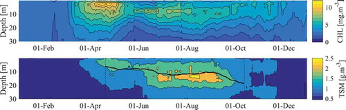
Figure 5. Typical examples of CHL profiles (top row), TSM profiles (middle row) and resulting R_rs (bottom row) for winter, spring, summer and autumn (left to right). The legend in the top left plot indicates the colour code for each simulation and in the bottom row the PD (%) and θ (°) values of M1, M5, GAL, TLM and LIN against INT.

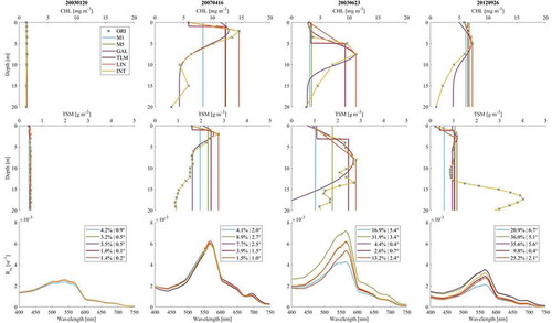
Figure 6. Seasonal evolution of the spectral angle for the uniform profiles M1 and M5 (top row) and for the three non-uniform approximation models GAL, TLM and LIN (bottom row).

Current inversion algorithms (e.g. those reviewed by Matthews, 2011; Odermatt et al., 2012) facilitate self-contained retrieval of water constituent concentrations from R_rs. Most of them are based on radiative transfer simulations, which are used directly as look-up tables for non-linear optimization (e.g. Van Der Woerd & Pasterkamp, 2008) and as training data for neural networks (e.g. Doerffer & Schiller, 2007), or indirectly for the parameterization of semi-analytical approximations such as Gordon et al. (1988). The extension of such simulations towards vertical non-uniformities requires a shape parameterization to enhance the comparability of measured and simulated R_rs. To minimize the dimensions of such look-up tables, the number of shape parameters should be small. Previous studies made use of the Gaussian shape approximation by Lewis, Cullen, and Platt (1983) in Stramska and Stramski (2005) or two-layer models (TLMs) (Yang et al., 2013b), and other representations such as a straight surface-to-peak gradient should be taken into consideration. An assessment of how appropriately they approximate R_rs for real vertical constituent distribution is needed, and the findings of this assessment must be traded off against the potential use of a priori knowledge, which could provide the needed shape parameters.

So far, due to obvious water quality issues, emphasis was put on eutrophic systems where most of the remote sensing optical information is limited to the top meter of the water column. Yet, the problem of retrieving information in lakes characterized by non-uniform vertical constituents applies to most oligo- to mesotrophic lakes that is most lakes on Earth. This study focuses on Lake Geneva as a well-documented example of a system with peaks of turbidity and chlorophyll from the surface to the deeper reaches of the photic layer. Our approach is meant to be directly applicable to any oligo- to mesotrophic lake.

Here, we investigate vertical non-uniformities and assess shape approximations using R_rs simulated for chlorophyll-a and turbidity profiles measured in Lake Geneva between 2002 and 2015. During this period, the Secchi depths varied in the range of 1–10 m, turbidity was between 0.4 and 4.6 Formazin Turbidity Units (FTU) and chlorophyll-a in the range of 0.8–17 mg m⁻³ for more than 95% of the profiles (plus a very few high exceptions of up to 10 FTU and 45 mg m⁻³, respectively). Lake Geneva is a partial monomictic lake with a seasonal thermal stratification representative for lakes in temperate climate zones, making this study representative for a wide range of mesotrophic lakes worldwide.

Methods

Site description

Lake Geneva is the largest natural freshwater lake of Western Europe with a surface area of 582 km² and a maximum depth of 310 m. It is situated between France and Switzerland and consists of two main water bodies, the deep Grand Lac and shallow Petit Lac (Figure 1). The Rhône River is the main tributary and the Rhône Valley is the largest part of its watershed. Minor contributors are the rivers Venoge and Aubonne in the north flowing down from the Jura and the Dranse in the south originating in the Alps. The only outflow is the Rhône River at Geneva on the western end of the lake. Lake Geneva became eutrophic in the 1970s largely due to increased human activities in the catchment (Rapin, Blanc, & Corvi, 1989). Extensive wastewater treatment, reduction of fertilizer use and law enforcement reduced nutrient inputs and improved water quality towards mesotrophic status (Anneville & Pelletier, 2000; Kiefer, Odermatt, Anneville, Wüest, & Bouffard, 2015). The first annual phytoplankton blooms generally occur close to the surface in spring, and their growth gradually moves towards deeper layers in the annual course (Dokulil & Teubner, 2012). Since 1957, the lake is regularly monitored by the Commission Internationale pour la Protection des Eaux du Léman (CIPEL) at two stations, SHL2 and GE3, in the Grand and Petit Lac, respectively.

Bio-geochemical constituents

Turbidity (TUR) and chlorophyll-a (CHL) profiles acquired at monitoring station SHL2 (Figure 1) between 2002 and 2015 that are available from SOERE OLA (INRA and CIPEL, 2016). The sampling frequency is fortnightly during the productive season between March and November, and monthly for the rest of the year. TUR profiles are sampled using different nephelometers and backscatter turbidity sensors according to the latest turbidity standard (ISO 7027-1, 2016): three Seapoint Turbidity Meters that measure FTU in the ranges of 0–1000 FTU (CTM214) and 0–2500 FTU (CTD009, CTD620) as well as an ECO-A sensor by ME Grisard (formerly ME Meerestechnik-Elektronik). The probes are lowered in the water by an electrical winch and profiles are inspected in real time. The turbidity found in Lake Geneva is only about 1% of the sensitivity range of the instruments; therefore, an averaging filter with a window size of 3 m is applied for noise reduction through outlier removal. Up to seven vertically consecutive records within no more than 3 m are clustered, and the central record is removed if its difference from the cluster’s median is larger than four times the interquartile range. Thirty-two out of a total of 11,000 records are removed by this procedure. We use TUR as equivalent to total suspended matter (TSM, in g m⁻³), according to findings for lakes, coastal and ocean waters (Bukata, Jerome, Bruton, & Bennett, 1978; Kallio, 2012; Neukermans, Ruddick, Loisel, & Roose, 2012). This correlation decreases with increasing particle diversity in riverine waters (Pfannkuche & Schmidt, 2003; Ruzycki, Axler, Host, Henneck, & Will, 2014), but is a fair approximation for pelagic lake sites like SHL2 (Figure 1). Water samples for CHL laboratory analysis are collected at nine depths, 0, 2.5, 5, 7.5, 10, 15, 20, 25 and 30 m, and processed according to the spectrophotometric method by Strickland-Parsons (1968) with regular quality and repeatability control. Given the impeccable quality of the CHL data, measurements are only excluded where no concurrent turbidity data is available. After quality control, the remaining 210 pairs of CHL(z) and TSM(z) are linearly interpolated to regular 10 cm vertical resolution, CHL(z_INT) and TSM(z_INT).

Vertical profile approximations

Five different models are applied for the approximation of vertical non-uniformities, including the Gaussian approximation according to Lewis et al. (1983; henceforth referred to as GAL, a k-means based TLM and a linear model (LIN). Using CHL(z_INT) and TSM(z_INT) profiles as input, the GAL model provides depth-dependent concentration B(z) according to Equation (1):

(1)

where B₀ is the background concentration, h is the vertical integral concentration in excess of B₀, z_max is the depth of maximum concentration B_max and σ quantifies the thickness of the layer with B > B₀. The TLM model provides for a layer boundary at z_l2 if z_l2 is neither zero nor below the maximum expected Secchi depth (i.e. 10 m) and with z_l2 the depth of the shoulder in the TLM as described below. After binary k-means classification of all CHL(z) and TSM(z) profiles in the range 0–15 m, the upper layer concentration is calculated as the median of all CHL(z) and TSM(z) with z < z_l2 that are not in the same class as B_max, and with z_l2 the depth of the shallowest point in the class of B_max. The lower layer concentration is set to the median of all CHL(z) and TSM(z) with z ≥ z_l2. The LIN model uses the same z_max as GAL and lower layer concentration B_max, according to the conclusions in Piskozub et al. (2008); for the upper layer a linear gradient is assumed between B(z = 0) and B(z_max). Finally, two profiles representing vertical uniformity are compiled for reference simulations by taking the median of CHL(z_INT) and TSM(z_INT) for the top 1 and 5 m (henceforth referred to as M1 and M5, respectively).

Radiometric measurements

Fifteen reflectance measurements acquired between 2014 and 2016 with a TriOS RAMSES system deployed in z = 1 m depth (Table 1) are used to verify the representativeness of the simulations for Lake Geneva. The extrapolation of in-water measurements towards and through the surface can be a considerable source of errors when striving for R_rs (Mueller & McClain, 2003). Therefore, R^– is preferred in this study because it is calculated from direct measurements at specific depths. Dimensionless irradiance reflectance R^– is derived according to Equation (2) from simultaneous measurements of up- and downwelling spectral irradiance, E_u and E_d respectively, at a sampling rate of 0.1 Hz during a 3 min run at 1 m depth:

(2)

Table 1. In situ campaigns conducted in Lake Geneva.

Date	Number of stations	Region
6 June 2014	3	Lausanne to SHL2
11 May 2015	9	Lausanne to SHL2
4 July 2015	1	SHL2
22 September 2016	2	Lausanne to SHL2

where and, in units of W m⁻² nm⁻¹, correspond to the median of the individual cast for each quantity over each run. The superscript ‘–’ refers to in-water measurements. For optical closure, reflectance R^– was sampled under cloud-free conditions (wind speed < 2 m s⁻¹) in 15 stations between Lausanne and SHL2 during the four campaigns listed in Table 1. Water depth was greater than three times the Secchi depth for all measurements, precluding bottom reflectance effects. At every station, 3.0 L of water was sampled at 0.5 m depth and stored in a dark cool box on the boat before filtration in the evening of each campaign. Two separate subsamples were filtered and stored at −40°C before analysis within a month for the following purpose: (i) CHL concentration was determined spectrophotometrically after 1.0 L of water was filtered through 0.8 µm GF/F filter papers and immersed in 99% ethanol for pigment extraction; (ii) 2.0 L was filtered to quantify TSM using gravimetric method on 0.8 µm pre-weighted and pre-combusted GF/F filters. Additional 100 mL of water was sampled at the same depth at 7 out of the 16 stations for the analysis of Coloured Dissolved Organic Matter (CDOM) absorption. 50 mL was filtered on-boat directly after sampling through 0.2 µm polycarbonate filters (Whatman Nuclepore) in dark glass vials stored in a cool box. The filters were pre-washed with consecutively 50 mL of Milli-Q water and 50 mL of water sample. In the evening after fieldwork, CDOM absorption was analysed using a dual-beam spectrophotometer.

Specific inherent optical properties

The bio-optical model shall be representative for Lake Geneva yet easily comparable to a larger number of optically complex waters. Like in comparable studies (Gholamalifard et al., 2013; Stramska & Stramski, 2005), specific inherent optical properties (SIOPs) remain fixed for all sampling dates and depths, which is owed to practical constraints but also favours the interpretability of the simulations. They are defined according to the simulations provided with IOCCG Report no. 5 (2006), other scientific publications and own measurements. Phytoplankton absorption (400–700 nm) normalized by (440 nm) = 0.05 m² mg⁻¹ is taken from Bricaud, Roesler, and Zaneveld (1995), which agrees quite well with long-term averaged coefficients for perialpine Lake Garda (Giardino et al., 2014). The 700–800 nm interval was added based on record 237 of the IOCCG data set, whose 675 nm peak agrees best with the Bricaud et al. (1995) absorption spectrum.

Phytoplankton scattering is neglected because the turbidity used for TSM(z) accounts for scattering by all particle types. Particle absorption is defined according to the exponential model in Equation (3) from the IOCCG Report no. 5 (2006):

(3)

where the subscript stands for non-algal particles and coefficients = 0.0146 nm⁻¹ and (440) = 0.025625 m² g⁻¹ are adopted again from IOCCG (2006) record 237, representing approximately median conditions when comparing to the variability of coefficients across the whole IOCCG data set. The same record is used for, which means the power law in Equation (4) is used with (550 nm) = 0.526255 m² g⁻¹ and m = 0.716:

(4)

Furthermore, the Fournier–Forand scattering phase function is used (Fournier & Forand, 1994), with a backscattering fraction b_b/b of 0.0183.

The spectral absorption of CDOM, a_CDOM, is approximated with Equation (5), whose parameters are estimated on the basis of irregular in situ measurements in Lake Geneva taken between 0 and 3 m of the water column.

(5)

For a_CDOM measurements acquired in parallel to the above-mentioned reflectance measurements, range and median of spectral slope γ are 0.010–0.018 and 0.014 nm⁻¹, respectively, which agrees with measurements in Lake Constance (Gege, 2000; Heege & Fischer, 2004), while for Lake Garda γ = 0.021 – 0.025 nm⁻¹ (Giardino, Brando, Dekker, Strömbeck, & Candiani, 2007; Giardino et al., 2014) are considerably higher. The range and median of the magnitude parameter across our measurements for Lake Geneva are 0.06–0.19 m⁻¹ and 0.12 m⁻¹, respectively. Simulations are carried out with fixed, vertically uniform m⁻¹ and slope (γ = 0.014 nm⁻¹) parameters because the monitoring data available from INRA-Thonon SOERE and CIPEL lack a suitable proxy for representing vertical non-uniformity in CDOM, and our subsurface measurements display rather stable conditions in the middle of the lake. Expected gradients in due to photobleaching near the surface (Del Vecchio & Blough, 2002) or alignment with the deep CHL maximum as observed in ocean waters (Green, Bower, & Lugo-Fernández, 2014; Yamashita et al., 2013) are likely to amplify uniformity effects, but they are not evident in the scarce measurements in Lake Geneva and rejected in order to err on the side of conservatism when it comes to non-uniformity effects on R_rs.

The absorption by pure water is derived with spectral spline fits using several sources for different wavelength ranges and resampled to 5 nm. From 350 to 550 nm, absorption by pure water is taken from Lee et al. (2015), and from 550 to 725 nm from Pope and Fry (1997) according to Pitarch, Volpe, Colella, Santoleri, and Brando (2016), and results by Smith and Baker (1981) are used for the range 725–800 nm (Pitarch, pers. comm). Scattering by pure water is computed at the resolution of its absorption using Zhang, Hu, and He (2009) relation with zero salinity and a water temperature of 15°C. Its phase function is taken from the Hydrolight model default file (pureh2o.dbf; see the following section for definition) with b_b/b = 0.5.

Radiative transfer model

Using the above-mentioned SIOPs, the Hydrolight 5.3 Radiative Transfer Model (Mobley, 1994; Mobley & Sundman, 2013) is applied to simulate R_rs for assessing the effect of different vertical approximation profiles. The solar zenith angle was set to 30°, wind speed is set to 2 m s⁻¹, clear-sky conditions are assumed for solar and sky irradiance calculations by the Hydrolight RADTRAN-X subroutine, and bottom reflectance effects are disabled.

Optical closure

The direct verification of bio-optical models with measured inherent and apparent optical properties requires comprehensive and accurate in situ measurements, in particular if vertical non-uniformities should be taken into account. Due to the lack of such measurements, we consider the approximation of several measured R^– with Hydrolight simulations at z = 1 m for uniform constituent gradients as sufficient evidence that the selected SIOPs are suitable for Lake Geneva. We use the Downhill-Simplex method (Nelder & Mead, 1965) with simultaneously measured CHL, TSM, as initial guess and minimizing the root mean squared error (RMSE) according to Equation (6) during fit iterations with the function fminsearch of the Matlab Optimization toolbox (Coleman, Branch, & Grace, 1999). Because CDOM was not measured at all stations, we used median in situ measurements of CDOM absorption at 440 nm in the initialization and was fixed using the median value of 0.012 nm⁻¹.

(6)

N enumerates wavelengths in 5 nm intervals between 405 and 705 nm, the subscripts meas and sim indicate simulated and measured reflectance spectra, respectively, and stands for any reflectance spectra under evaluation (in this study either R^– or R_rs).

Statistics

The per cent difference (PD) [%] is used to assess the differences between measured and simulated spectra, or between different approximation models, defined at every wavelength as

(7)

This metric in per cent allows exhibiting the similarities between spectra R₁ and R₂ in terms of amplitude. The larger the PD value, the more distant are the spectra R₁ and R₂. On the other hand, the spectral shape difference is assessed using the spectral angle (), defined as (Dennison, Halligan, & Roberts, 2004; Xue et al., 2015)

(8)

The term varies between 0° and 90°, with 0° meaning similar spectra and larger showing increasing dissimilarities.

Inversion algorithms

For evaluating the impact of non-uniformities on inversion algorithms, we apply band ratio-based algorithms that use R_rs in different spectral regions. First, the standard Ocean Colour OC4 band ratio is tested, which uses the blue and green region of the spectra with the general form:

(9)

where coefficients are taken from Werdell and Bailey (2005) for use of the MERIS sensor, and R_rs were convolved using MERIS bands’ specific spectral response. The numerator,, in OC4 is the maximum of MERIS bands 2, 3 and 4 (centred at 443, 490 and 510 nm, respectively) over the green band 5 (centred at 560 nm).

The second algorithm used was developed by Gons (2002, 2005)) and is henceforth referred to as GONS. It is a semi-analytic algorithm that uses the red near-infrared (red-NIR) region of the spectra as

(10)

where R_M is the ratio between MERIS bands 9 to 7 (centred at 709 and 665 nm, respectively) of R_rs. Again R_rs was convolved to MERIS bands. The term b_b stands for the backscattering coefficient (m⁻¹) derived in the original algorithm using MERIS band 12 (centred at 779 nm) according to

(11)

Results

Optical closure

Across all 15 radiometric measurements, the median PD between measured and optimized R^– in the wavelength range between 405 and 700 nm is 4.7%, and it is always lower than 24% with larger median PD occurring around 565 nm, and a larger spread occurring above 610 nm (Figure 2). The optimization of reflectance magnitudes in blue and red wavelengths is a trade-off because most IOPs come with large magnitude differences between these two wavelength regions. At the same time the euphotic depth for blue light is much larger than for red, and therefore potential non-uniformity effects in the measured R^– complicate the interpretation of the uneven PD level. However, the agreement of spectral shapes between 600 and 700 nm is quite good, indicating that the selected pigment absorption from Bricaud et al. (1995) has an appropriate secondary peak, even though it may be responsible for a small spectral shape bias around 565 nm (Figure 2). Specifically, this bias might influence the result of inversion algorithm which involves this region of the spectra in its calculation. In fact, we observe that optimized values of CHL and TSM are systematically lower and higher, respectively (Table 2), and the use of such IOPs for water quality monitoring must be treated with care. For the three examples in Figure 3, initial and optimized concentrations of CHL, TSM and CDOM are given in Table 2 along with minimum and maximum for all simulations. The disagreement is considerable, but still in the range of expected measurement uncertainties and within the non-uniformity effects demonstrated hereafter. Hence we consider the selected set of SIOPs representative for our simulation study.

Table 2. Water constituents parameters used in the optical closure.

Station	Initial concentrations			Optimized concentrations
	CHL (mg m^−3)	TSM (g m^−3)	(m^−1)	CHL (mg m^−3)	TSM (g m^−3)	(m^−1)
1	4.1	0.8	0.12	2.6	1.4	0.15
6	18	3.0	0.12	12.7	3.2	0.07
8	2.0	1.5	0.12	1.2	1.7	0.06
Min.	1.8	0.5	0.12	0.8	0.7	0.03
Max.	18	4.4	0.12	13.4	4.7	0.13

Note: CHL and TSM are near-surface measurements, while a long-term average is used as initial guess for a_CDOM.

Average annual course of constituent non-uniformities

The average annual course of vertical CHL and TSM non-uniformities in the centre of Lake Geneva corresponds roughly to the four climatic seasons (Figure 4). In most years a clear-water phase in winter is subject to low and vertically uniform concentrations in both CHL and TSM, peaking around 4 mg m⁻³ and 1 g m⁻³, respectively. Around the second half of March, spring blooms develop in the top 5 m of the water column, with maximum CHL concentrations between 10 and 20 mg m⁻³. It must be considered that the chance of fortnightly samples representing the actual spring peak in Lake Geneva is low (Kiefer et al., 2015), but CHL levels often remain around 10 mg m⁻³ for several weeks during this period. In summer, productivity decreases and the CHL maximum descends to 10–20 m depth due to the depletion of nutrients in the epilimnion and the supply by riverborne nutrients in the thermocline. The fall season is marked by a transition in phytoplankton assemblage with species more adapted to low insolation and mixed water column conditions characterized by lower CHL concentrations compared to the first phytoplankton bloom of the year. The seasonal turbidity peak in the thermocline largely results from the fine glacial inorganic particles transported by the Rhône River and trapped in the thermocline where riverine water typically intrudes during summer (Bouffard & Perga, 2016; Finger, Schmid, & Wüest, 2006).

Vertical approximation of seasonally typical profiles

The vertical non-uniformities in CHL and TSM have seasonally specific effects on R_rs (Figure 5). In winter, the approximation of the constituent’s fairly uniform vertical distributions is as simple as redundant, even though the highest light penetration depths occur in this season. Contrariwise, near-surface phytoplankton blooms in spring reduce the euphotic depth in all wavelengths. Non-uniformities develop quickly in the top few meters of CHL profiles, but less so in turbidity profiles. Accordingly, the divergence of R_rs simulations for different profile approximations affects predominantly wavelengths with pigment absorption when phytoplankton distribution is assumed to extend to the very surface, as shown for M5 and GAL in the example of 16 April 2007 (Figure 5). As non-uniformities in turbidity amplify throughout the productive season, magnitude differences increase. At the same time, the descent of the CHL peak beyond the euphotic depth of red-NIR wavelengths also constrains that R_rs remains representative of a relatively homogeneous upper mixed layer while the most productive layer becomes inaccessible at these wavelengths, e.g. when comparing the alignment of the secondary CHL absorption band at 665 nm for M1 and TLM on 23 June 2003. The breakup of stratification in autumn brings about a variety of different vertical constituent distributions, ranging from a steady fading towards uniformity in some years, to short-term, near-surface phytoplankton blooms with potentially large effects in other years (e.g. 26 September 2012).

Henceforth, we investigate the appropriateness of profile approximation models by comparing Hydrolight simulated R_rs for the five profiles M1, M5, GAL, LIN and TLM with the simulations for the corresponding measured profiles (INT). In the bottom row of Figure 5 R_rs spectra are compared and and PD are shown as measures of spectral offset.

Frequency and temporal distribution of non-uniformities

The temporal distribution of for each of the five approximation models for the years 2002–2015 provides an overview of the relevance of vertical non-uniformities (Figure 6). First we consider M1 and M5, where > 3° for roughly half of the profiles between May and September. The maximum values occur in July with > 5° for roughly half and one-third of profiles approximated by M1 and M5, respectively. During the rest of the year, the deviations are generally low even in early spring, which confirms the representativeness of the examples chosen in Figure 5. This means that the overall frequency of cases with > 5° is low (20% and 9% for M1 and M5, respectively), but these cases cause strong uncertainty during the productive season, which is underestimated when considered only as arithmetic means or medians.

The other three non-uniformity approximation models show significantly lower than M1 and M5 (Figure 6, bottom row). Their spectral match with INT reference R_rs is significantly higher during the productive season, in spite of occasional limitations. In general, GAL and TLM show smallest deviations from the observational estimates. They both provide for a homogeneous surface layer and concentration increases along a more or less sharp layer boundary, as opposed to LIN, which assumes that concentrations increase steadily. TLM’s main limitation is that such steady increases still occasionally occur in the measurements, while TLM always defines a sharp boundary. This is less the case with GAL, which simulates perfectly large bell-shaped profiles, but fails when there is a strong gradient at the surface. Maximum observed for TLM and GAL are 6.3° and 9.3°, respectively.

Assessment of profile approximation models

The performance of the considered approximations depends on the range of the euphotic depths for the different wavelengths during the course of the year, and the approximations’ ability to reproduce the constituent concentrations at these depths. This is most obvious for vertically uniform profiles M1 and M5, which are quite appropriate when euphotic depths are in the order of ~1 and ~5 m, respectively, but much less in the other spectral regions (Figure 7, left). Accordingly, maximum spectral PD of these two non-uniform approximations vary strongly and almost contrariwise, while the median PD of M5 at 400–590 nm is relatively constant.

Figure 7. Maximum PD (top row) and median PD (bottom row) over all simulations for INT input profiles against the uniform (left) and non-uniform profile approximation models (right).

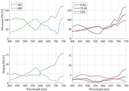
The accuracy of the GAL, LIN and TLM approximation models is illustrated on the right panel of Figure 7. We note that GAL PD distribution is similar to M5 with generally better performances from the former by a factor between 1.5 and 2.0 and it is the model which performs best in the green region, where the maximum PD reaches only 26% around 560 nm. TLM and LIN have both very similar performances with maximum PD increasing between 400 and 550 nm from 30% to 64%. However, the median of TLM is significantly lower varying between 2% to 3% in the same region against 3% to 6% for LIN. In the red the median PD for both model remains relatively low and the differences between them decrease whereas maximum values increase from 50% at 600 nm to >100% at 750 nm.

The score for each model in Table 3 shows that M1 performs significantly worse when it comes to the spectral shape as is the case for magnitudes and the PD (Figure 7). The non-uniformity models achieve again a significantly better agreement with INT, with rather insignificant differences between GAL, TLM and LIN.

Table 3. Median and maximum spectral angles between INT and individual approximation models over all simulations.

(°)	M1	M5	GAL	TLM	LIN
Median	1.96	1.53	0.65	0.67	0.62
Maximum	15.9	12.4	9.3	6.3	8.6

Relative relevance of CHL and TSM

The relative importance of vertical non-uniformities in CHL(z) and TSM(z) is of particular interest given that their vertical gradients are independent. When comparing M1 and M5 for 16 April 2007 and 23 June 2003 (Figure 5), we note that the difference in CHL (8.35 and 12.35 mg m⁻³, respectively) prevails in spring, while the difference in TSM (1.03 and 1.78 g m⁻³, respectively) prevails in summer. The PD for the former are considerably lower than for the latter, even though the non-uniformities are closer to the surface in spring. A number of similar examples suggest that TSM variations have a considerably larger effect on PD. In order to test this hypothesis on our entire data set, we investigate the relation between the CHL and TSM variations and the PD between 400 and 700 nm. To get the difference of either CHL or TUR between two different simulations, we use M1 and M5 profiles because their difference yields a single scalar. After visual inspection, a log–log relation was selected. For TSM, we found a significant relation (p < 1 × 10⁻¹⁰) at all wavelengths with R² minimum in the blue range (R² = 0.3) and steadily increasing until the red at 650 nm (R² = 0.8). Those results suggest that a non-linear relation exist between the TSM differences of two profiles and the PD between the resulting R_rs. The large R² values imply that TSM difference explains a significant amount of variations in the amplitude of the reflectance. For CHL, the null hypothesis can be rejected only around 550 nm (p > 0.15) although in the rest of the spectra R² is always <0.05. As expected, the CHL difference cannot explain a significant part of the variations in PD.

In order to see the direct relation of CHL and TSM on the shape of the R_rs spectra rather than the amplitude, we conducted the same experiment using instead of the average PD as response variable. Using both p-values are almost equal to 0 and give R² of 0.27 and 0.39 for TSM and CHL, respectively, showing that both TSM and CHL have a significant impact on the shape of the spectra with the latter being more significant.

Band ratio algorithm

The effects of vertical non-uniformities on water constituent retrieval algorithms are complex and require individual clarification. As indicative example for expected retrieval errors, we compare CHL retrieved from vertically non-uniform INT simulations with CHL for the corresponding M1 and M5. Non-uniformities affect the retrieval accuracy of the algorithms and the representativeness of their sensing depth. We investigate both aspects using OC4 and GONS algorithms. Both algorithms have known limitations for processing remote sensing imagery of Lake Geneva. The use of OC4 is impaired by independently varying CDOM and TSM concentrations, and water-leaving radiance and CHL levels are usually too low for robust retrieval from red-NIR reflectance as with GONS. In the case of our factitious simulations, neither effects due to CDOM variations nor uncertainties in R_rs at red-NIR wavelengths must be expected, leaving OC4’s TSM sensitivity and weak performance of GONS at low CHL levels (see Gons, Auer, & Effler, 2008; Figure 2) as sole inconsistency. As implied by PD in the red for M1 in Figure 7, the GONS for INT and M1 are highly correlated in spite of the poor sensitivity of the algorithm for low CHL concentrations (Figure 8, R² = 0.89). This confirms that red-NIR algorithms are almost unaffected by vertical uniformities at least as far as vertical scales resolved by standard in situ measurements are concerned. However, the restriction on red-NIR wavelengths with minimal penetration depth also means that red-NIR algorithms can resolve near-surface phenomena like spring blooms, while they cannot access relevant dynamics at 5–10 m depth in the second half of the year. On the contrary, for OC4 the correlation between INT and M5 (R² = 0.46) is slightly higher than that between INT and M1 (R² = 0.4). And, given the potential impact of a few outliers on the determination coefficient, the alignment along the 1:1 line is much better, confirming that the OC4 algorithm has a sensing depth that is overall closer to 5 m than to 1 m.

Figure 8. Scatter plot of GONS (top row) and OC4 (bottom row) algorithms applied on M1 (left) and M5 (right) against R_rs from measured CHL(z). The grey line represents the 1:1 relationship and the black line represents the regression with the resulting slope and R² provided in the text box of each plot. Note that a log–log scale is applied to cope with the scatter of OC4 samples while a lin–lin scale is required to display the negative values in GONS.

Discussion and conclusions

Our findings suggest a number of practical implications for water quality remote sensing of oligo- to mesotrophic lakes, which represent the global majority. These implications concern effects of non-uniformity on retrieval accuracy, the relevance of different sensing depths across the visible and near-infrared spectrum, and the integration of vertical non-uniformities in invertible bio-optical models.

In standard water quality remote sensing validation, retrieval results from (atmospherically corrected) R_rs of vertically non-uniform profiles are compared to vertically explicit or averaged water constituent concentration measurements. The comparisons in Figure 8 emulate such a validation by comparing retrieval results from R_rs of vertically non-uniform profiles and those from R_rs of constant vertical concentration profiles. The resulting R² and sample alignment are slightly better than in typical validation exercises for similar lakes (e.g. Odermatt, Giardino, & Heege, 2010), even though significant error sources are ineffective (CDOM, sensor noise, atmospheric correction). We found that about 20% of the 210 samples in our data set are affected by significant non-uniformities (INT compared to M1, > 5°). This means that together with other limitations, such as different horizontal sampling locations (e.g. Moses, Ackleson, Hair, Hostetler, & Miller, 2016) and related variations in IOPs (e.g. Babin, Morel, Fournier-Sicre, Fell, & Stramski, 2003), vertical non-uniformities are a major obstacle to provide accurate remote sensing products in oligo- to mesotrophic lakes.

Based on this first conclusion, we argue further that the increasing popularity of red-NIR algorithms is supported by their minimal sensitivity to vertical non-uniformities. Using adjacent wavelengths with similar and low penetration depths, such algorithms retain robustness and comparability to surface samples even where non-uniformities occur. However, given that only a relatively small part of the annual primary productivity and other relevant near-surface processes in oligo- and mesotrophic waters occur in the top 1 m of the water column (Figure 4), the usage of such algorithms implies that a significant amount of these processes remain unnoticed. On the other hand, we conclude that algorithms using larger portions of the reflective spectrum suffer much more from differences in light penetration depth due to vertical non-uniformities.

Developing retrieval algorithms that account for non-uniformities introduces the challenge of an increased number of unknown parameters. In this regard, we observed that vertical non-uniformities in TSM have a larger effect on R_rs than those in CHL, and that the vertical gradients in TSM and CHL are independent. When it comes to the approximation of those vertical gradients, GAL requires four shape parameters (B₀, z_max, h and σ) and approximates the entire gradient across the defined 10 m depth. On the contrary, TLM and LIN require only three shape parameters to approximate the upper and more relevant side of approximately bell-shaped constituent gradients. Based on the performance assessment in Figure 7 and Table 3, the TLM is best suited to produce realistic R_rs for algorithm development.

Further research is required to relate predictable stratification indicators, such as thermocline depth (Figure 4), to the TLM layer boundary of vertical constituent distributions, and hence create applicable a priori information for inversion procedures. Specifically, we aim to compile a look-up table that accounts for non-uniformities and which can be searched by means of model-derived a priori knowledge. Based on promising results from validation and long-term analyses of remotely sensed chlorophyll-a concentrations (Kiefer et al., 2015), a hydrodynamic model for the lake (Razmi et al., 2013, 2014) is in further development to provide near-real-time estimates of mixing layer depth and other physical parameters as potential input for remote sensing methods (http://meteolakes.ch). In addition, it should be investigated whether analogous effects can be observed for near-surface CDOM gradients due to photo-degradation.

In summary, we demonstrated the need to account for vertical inhomogeneity in CHL and TSM for correctly analysing remote sensing reflectance in oligo- to mesotrophic lakes, which show characteristic non-uniformities to significant depth. This work is part of an attempt to better connect remotely sensed observations with hydrodynamic and water quality modelling. While the former typically provides information for validation of the latter, the latter can also be used to provide ancillary information to better constrain the classical ill-posed inverse retrieval procedures. It is through such activity of coupling various sources of information that breakthrough solution will be provided for lake ecosystem understanding and monitoring.

Acknowledgments

The authors thank François Bernard, José Couttet and the Russian ULM pilots for their excellent performance. They also thank the Limnology Center at EPFL, in particular Jean-Denis Bourquin, Ulrich Lemmin and Natacha Pasche for project coordination and administration. The assistance of Mikhail Krasnoperov (Consulat Honoraire de la Fédération de Russie) as liaison is greatly appreciated. For the CIPEL data, Frédéric Soulignac and Orlane Anneville provided reliable support. The authors also gratefully acknowledge Tiit Kutser, Koponen Sampsa and Peter Gege for their comments and help to improve the manuscript as well as all members of the APHYS laboratory (EPFL) for their contribution during fieldwork and long-lasting support.

Disclosure statement

No potential conflict of interest was reported by the authors.

Additional information

Funding

This work was supported by the Fondation pour l’Etude des Eaux du Léman (FEEL) on Lake Geneva; Margaretha Kamprad Chair; Dr. Paulsen Foundation Inc.; Council Foundation for Baikal Protection on Lake Baikal.

References

- Anneville, O., & Pelletier, J.P. (2000). Recovery of Lake Geneva from eutrophication: Quantitative response of phytoplankton. Archives Für Hydrobiol - Hauptbände, 148, 607–624.
- Babin, M., Morel, A., Fournier-Sicre, V., Fell, F., & Stramski, D. (2003). Light scattering properties of marine particles in coastal and open ocean waters as related to the particle mass concentration. Limnology and Oceanography, 48, 843–859.
- Bouffard, D., & Perga, M.-E. (2016). Are flood-driven turbidity currents hot spots for priming effect in lakes? Biogeosciences (Online), 13, 3573–3584.
- Bricaud, A., Roesler, C., & Zaneveld, J.R.V. (1995). In situ methods for measuring the inherent optical properties of ocean waters. Limnology and Oceanography, 40, 393–410.
- Bukata, R.P., Jerome, J.H., Bruton, J.E., & Bennett, E. (1978). Relationship among optical transmission, volume reflectance, suspended sediment concentration, and chlorophyll-a concentration in Lake Superior. Journal of Great Lakes Research, 4, 456–461.
- Churnside, J.H. (2015). Bio-optical model to describe remote sensing signals from a stratified ocean. Journal Applications Remote Sens, 9(1), 095989.
- Coleman, T., Branch, M.A., & Grace, A. (1999). Matlab optimization toolbox user’s guide (3rd ed.). Natick: Math Works.
- Curtarelli, M.P., Ogashawara, I., Alcântara, E.H., & Stech, J.L. (2015). Coupling remote sensing bio-optical and three-dimensional hydrodynamic modeling to study the phytoplankton dynamics in a tropical hydroelectric reservoir. Remote Sensing of Environment, 157, 185–198.
- Del Vecchio, R., & Blough, N.V. (2002). Photobleaching of chromophoric dissolved organic matter in natural waters: Kinetics and modeling. Mar Chemical, 78, 231–253.
- Dennison, P.E., Halligan, K.Q., & Roberts, D.A. (2004). A comparison of error metrics and constraints for multiple endmember spectral mixture analysis and spectral angle mapper. Remote Sensing of Environment, 93, 359–367.
- Doerffer, R., & Schiller, H. (2007). The MERIS Case 2 water algorithm. International Journal Remote Sens, 28, 517–535.
- Dokulil, M.T., & Teubner, K. (2012). Deep living Planktothrix rubescens modulated by environmental constraints and climate forcing. Hydrobiologia, 698, 29–46.
- Erga, S.R., Ssebiyonga, N., Hamre, B., Frette, Ø., Hovland, E., Hancke, K., Rey, F. (2014). Environmental control of phytoplankton distribution and photosynthetic performance at the Jan Mayen Front in the Norwegian Sea. Journal Mar Systems, 130, 193–205.
- Finger, D., Schmid, M., & Wüest, A. (2006). Effects of upstream hydropower operation on riverine particle transport and turbidity in downstream lakes. Water Resources Researcher, 42(8), W08429.
- Fournier, G.R., & Forand, J.L. (1994). Analytic phase function for ocean water. Proceedings of the SPIE, 2258, 194–201.
- Gege, P. (2000, October). Gaussian model for yellow substance absorption spectra. In Proc. Conference of Ocean Optics XV, Monaco.
- Gholamalifard, M., Esmaili-Sari, A., Abkar, A., Naimi, B., & Kutser, T. (2013). Influence of vertical distribution of phytoplankton on remote sensing signal of Case II waters: Southern Caspian Sea case study. Journal Applications Remote Sens, 7(1), 073550.
- Giardino, C., Brando, V.E., Dekker, A.G., Strömbeck, N., & Candiani, G. (2007). Assessment of water quality in Lake Garda (Italy) using Hyperion. Remote Sensing Environment, 109, 183–195.
- Giardino, C., Bresciani, M., Cazzaniga, I., Schenk, K., Rieger, P., Braga, F., Brando, V. (2014). Evaluation of multi-resolution satellite sensors for assessing water quality and bottom depth of Lake Garda. Sensors, 14, 24116–24131.
- Gons, H.J. (2002). A chlorophyll-retrieval algorithm for satellite imagery (Medium Resolution Imaging Spectrometer) of inland and coastal waters. Journal of Plankton Research, 24, 947–951.
- Gons, H.J. (2005). Effect of a waveband shift on chlorophyll retrieval from MERIS imagery of inland and coastal waters. Journal of Plankton Research, 27, 125–127.
- Gons, H.J., Auer, M.T., & Effler, S.W. (2008). MERIS satellite chlorophyll mapping of oligotrophic and eutrophic waters in the Laurentian Great Lakes. Remote Sensing Environment, 112, 4098–4106.
- Gordon, H.R., Brown, O.B., Evans, R.H., Brown, J.W., Smith, R.C., Baker, K.S., & Clark, D.K. (1988). A semianalytic radiance model of ocean color. Journal of Geophysical Research, 93, 10909–10924.
- Gordon, H.R., & McCluney, W.R. (1975). Estimation of the depth of sunlight penetration in the sea for remote sensing. Applications Optical, 14, 413–416.
- Green, R.E., Bower, A.S., & Lugo-Fernández, A. (2014). First Autonomous Bio-Optical Profiling Float in the Gulf of Mexico reveals dynamic biogeochemistry in deep waters. PLOS ONE, 9, e101658.
- Heege, T., & Fischer, J. (2004). Mapping of water constituents in Lake Constance using multispectral airborne scanner data and a physically based processing scheme. Canada Journal Remote Sens, 30, 77–86.
- INRA, & CIPEL (2016). Long-term Observation and Experimentation System for Environmental Research - Alpine Lake Observatory (SOERE-OLA). www.si-ola.inra.fr, accessed 22 November 2016.
- IOCCG. (2006). Remote sensing of inherent optical properties: fundamentals, tests of algorithms, and applications. In Z.-P. Lee ed., Reports of the International Ocean-Colour Coordinating Group, No. 5. Dartmouth, Canada: Author.
- ISO 7027-1 (2016). Water quality - Determination of turbidity - Part 1: Quantitative methods.
- Kallio, K. (2012). Water quality estimation by optical remote sensing in boreal lakes (Doctoral dissertation). University of Helsinki, Helsinki, Finland.
- Kiefer, I., Odermatt, D., Anneville, O., Wüest, A., & Bouffard, D. (2015). Application of remote sensing for the optimization of in-situ sampling for monitoring of phytoplankton abundance in a large lake. The Science of the Total Environment, 527–528, 493–506.
- Kutser, T., Metsamaa, L., & Dekker, A.G. (2008). Influence of the vertical distribution of cyanobacteria in the water column on the remote sensing signal. Estuar Coast Shelf Sciences, 78, 649–654.
- Lee, J.-Y., Kim, J.-K., Owen, J.S., Choi, Y., Shin, K., Jung, S., & Kim, B. (2013). Variation in carbon and nitrogen stable isotopes in POM and zooplankton in a deep reservoir and relationship to hydrological characteristics. Journal Freshw Ecology, 28, 47–62.
- Lee, Z., Wei, J., Voss, K., Lewis, M., Bricaud, A., & Huot, Y. (2015). Hyperspectral absorption coefficient of “pure” seawater in the range of 350–550 nm inverted from remote sensing reflectance. Applications Optical, 54(3), 546–558.
- Lewis, M.R., Cullen, J.J., & Platt, T. (1983). Phytoplankton and thermal structure in the upper ocean: Consequences of nonuniformity in chlorophyll profile. Journal Geophys Researcher Oceans, 88, 2565–2570.
- Matthews, M.W. (2011). A current review of empirical procedures of remote sensing in inland and near-coastal transitional waters. International Journal Remote Sens, 32, 6855–6899.
- McCulloch, A.A., Kamykowski, D., Morrison, J.M., Thomas, C.J., & Pridgen, K.G. (2013). A physical and biological context for Karenia brevis seed populations on the northwest Florida shelf during July 2009. Cont Shelf Researcher, 63, 94–111.
- Mobley, C.D. (1994). Light and water. San Diego, USA: Academic Press.
- Mobley, C.D., & Sundman, L.K. (2013). HydroLight 5.2 - EcoLight 5.2 technical documentation. Bellevue, United States: Sequoia Scientific, Inc.
- Montes-Hugo, M.A., Churnside, J.H., Gould, R.W., Arnone, R.A., & Foy, R. (2010). Spatial coherence between remotely sensed ocean color data and vertical distribution of lidar backscattering in coastal stratified waters. Remote Sensing Environment, 114, 2584–2593.
- Moses, W.J., Ackleson, S.G., Hair, J.W., Hostetler, C.A., & Miller, W.D. (2016). Spatial scales of optical variability in the coastal ocean: Implications for remote sensing and in situ sampling. Journal Geophys Researcher Oceans, 121, 4194–4208.
- Mueller, J.L., & McClain, C. NASA. (2003). Ocean optics protocols for satellite ocean color sensor validation, revision 4, vol. III: Radiometric measurements and data analysis protocols. Maryland: Greenbelt.
- Nelder, J.A., & Mead, R. (1965). A simplex method for function minimization. Computation Journal, 7, 308–313.
- Neukermans, G., Ruddick, K., Loisel, H., & Roose, P. (2012). Optimization and quality control of suspended particulate matter concentration measurement using turbidity measurements. Limnol Oceanogr Methods, 10, 1011–1023.
- Odermatt, D., Giardino, C., & Heege, T. (2010). Chlorophyll retrieval with MERIS Case-2-Regional in perialpine lakes. Remote Sensing Environment, 114, 607–617.
- Odermatt, D., Gitelson, A., Brando, V.E., & Schaepman, M.E. (2012). Review of constituent retrieval in optically deep and complex waters from satellite imagery. Remote Sensing Environment, 118, 116–126.
- Pfannkuche, J., & Schmidt, A. (2003). Determination of suspended particulate matter concentration from turbidity measurements: Particle size effects and calibration procedures. Hydrol Processing, 17, 1951–1963.
- Piskozub, J., Neumann, T., & Wozniak, L. (2008). Ocean color remote sensing: Choosing the correct depth weighting function. Optical Express, 16, 14683–14688.
- Pitarch, J., Odermatt, D., Kawka, M., & Wüest, A. (2014). Retrieval of vertical particle concentration profiles by optical remote sensing: A model study. Optical Express, 22(S3), A947−A959.
- Pitarch, J., Volpe, G., Colella, S., Santoleri, R., & Brando, V. (2016). Absorption correction and phase function shape effects on the closure of apparent optical properties. Applications Optical, 55, 8618–8636.
- Pope, R.M., & Fry, E.S. (1997). Absorption spectrum (380–700 nm) of pure water. II. Integrating cavity measurements. Applications Optical, 36, 8710–8723.
- Rapin, F., Blanc, P., & Corvi, C. (1989). Influence des apports sur le stock de phosphore dans le lac Léman et sur son eutrophisation. Reviews Sciences Eau, 2, 721–737.
- Razmi, A.M., Barry, D.A., Bakhtyar, R., Le Dantec, N., Dastgheib, A., Lemmin, U., & Wüest, A. (2013). Current variability in a wide and open lacustrine embayment in Lake Geneva (Switzerland). Journal Gt Lakes Researcher, 39, 455–465.
- Razmi, A.M., Barry, D.A., Lemmin, U., Bonvin, F., Kohn, T., & Bakhtyar, R. (2014). Direct effects of dominant winds on residence and travel times in the wide and open lacustrine embayment: Vidy Bay (Lake Geneva, Switzerland). Aquat Sciences, 76(Suppl 1), S59–S71.
- Ruzycki, E.M., Axler, R.P., Host, G.E., Henneck, J.R., & Will, N.R. (2014). Estimating sediment and nutrient loads in four Western Lake Superior streams. JAWRA Journal American Water Resources Association, 50, 1138–1154.
- Ryan, J.P., Davis, C.O., Tufillaro, N.B., Kudela, R.M., & Gao, B.-C. (2014). Application of the Hyperspectral Imager for the oastal ocean to phytoplankton ecology studies in Monterey Bay, CA, USA. Remote Sensing, 6, 1007–1025.
- Smith, R.C., & Baker, K.S. (1981). Optical properties of the clearest natural waters (200–800 nm). Applications Optical, 20(2), 177–184.
- Stramska, M., & Stramski, D. (2005). Effects of a nonuniform vertical profile of chlorophyll concentration on remote-sensing reflectance of the ocean. Applications Optical, 44, 1735–1747.
- Strickland, J.D.H., & Parsons, T.R. (1968). A practical handbook of seawater analysis (pp. 167). Canada, Bull. Fish. Res. Board.
- Van Der Woerd, H.J., & Pasterkamp, R.H. (2008). HYDROPT: A fast and flexible method to retrieve chlorophyll-a from multispectral satellite observations of optically complex coastal waters. Remote Sensing Environment, 112(4), 1795–1807.
- Werdell, P.J., & Bailey, S.W. (2005). An improved in-situ bio-optical data set for ocean color algorithm development and satellite data product validation. Remote Sensing Environment, 98, 122–140.
- Xue, K., Zhang, Y., Duan, H., Ma, R., Loiselle, S., & Zhang, M. (2015). A remote sensing approach to estimate vertical profile classes of phytoplankton in a Eutrophic Lake. Remote Sensing, 7, 14403–14427.
- Yamashita, Y., Nosaka, Y., Suzuki, K., Ogawa, H., Takahashi, K., & Saito, H. (2013). Photobleaching as a factor controlling spectral characteristics of chromophoric dissolved organic matter in open ocean. Biogeosciences (Online), 10, 7207–7217.
- Yang, Q., Stramski, D., & He, M.-X. (2013). Modeling the effects of near-surface plumes of suspended particulate matter on remote-sensing reflectance of coastal waters. Applications Optical, 52, 359–374.
- Zaneveld, J.R.V., Barnard, A.H., & Boss, E. (2005). Theoretical derivation of the depth average of remotely sensed optical parameters. Optical Express, 13, 9052–9061.
- Zhang, X., Hu, L., & He, M.-X. (2009). Scattering by pure seawater: Effect of salinity. Optical Express, 17(7), 5698–5710.