Assessment of values and trends in coarse spatial resolution NDVI datasets in Southeast Asia landscapes

ABSTRACT

Normalized difference vegetation index (NDVI) has been widely applied for monitoring vegetation dynamics. However, NDVI values are known to be profoundly affected by various external factors. In this study, the variation of NDVI values and trends among the several long-term NDVI datasets with resolution of 1, 4 and 8 km were assessed to understand the differences between the available datasets. The assessment items were 1) Pearson’s correlation coefficient, 2) trend map and breakpoint spatial similarities and 3) comparison of NDVI from Landsat and Flux tower in 2007–2015. The comparison revealed a maximum correlation coefficient of 0.67 among NDVI datasets and average spatial similarity of 37.2% among the trend maps estimated from NDVI datasets. Furthermore, there was a possibility of having significantly opposite trends between two trend maps from different NDVI products. Comparisons with NDVI from vegetation pixel in Landsat 5 TM and 8 OLI resulted in the R² between 0.06 and 0.68 and RMSE of 0.07–0.2, while comparison with NDVI from flux tower data yielded the RMSE of 0.04–0.41, although the R² was relatively weak at 0–0.18. Our study highlights the possibility of differences among NDVI datasets, and suggests that these differences should be reconciled especially in time-series analysis.

KEYWORDS:

• Pairwise correlation
• trend assessment
• breakpoint analysis
• spatial similarity

Introduction

Monitoring and measuring the vegetation over large areas using satellite remote sensing has frequently been performed. To correlate values obtained by satellite imaging with actual vegetation characteristics, vegetation indices were developed as spectral transformations that mostly utilize the red and infrared bands, which are sensitive to leaf pigments. Among the different vegetation indices, one index that has been widely used for long-term datasets is the normalized difference vegetation index (NDVI). NDVI can be used to analyze various aspects of vegetation such as vegetation dynamics, productivity and the effects of climate on vegetation, allowing mapping of the spatial and temporal distributions of vertical and horizontal structures such as vegetation community and vegetation biomass (Pettorelli et al., 2005) and land cover mapping (Defries & Townshend, 1994).

NDVI has been viewed as a proxy for vegetation greenness and has been widely used for predicting biophysical properties of vegetation such as the leaf area index (LAI) (Turner, Cohen, Kennedy, Fassnacht, & Briggs, 1999; Wang, Adiku, Tenhunen, & Granier, 2005) and the fraction of photosynthesis active radiation (FAPAR) (Myneni & Williams, 1994) across different vegetation landscapes. Although NDVI has been successfully applied, the values are known to be sensitive to external factors such as soil and canopy background, atmospheric disturbances, and sun-sensor viewing angle (Baret & Guyot, 1991; Epiphanio & Huete, 1995; Myneni & Williams, 1994; Roujean, Leroy, & Deschamps, 1992). Moreover, application of NDVI in areas with dense vegetation results in signal saturation, particularly for LAI values above 2–3 (Carlson & Ripley, 1997), and thus makes it less likely to provide accurate information of biophysical features vegetation and phenology in this particular area.

While instantaneous NDVI values are also susceptible to the same problems, time series NDVI observations are sensitive to sensor changes, especially when data from several satellite missions are used to construct the time series observations, particularly in advanced very high-resolution radiometer (AVHRR)-based NDVI data and to orbital drift, which affects the solar zenith angle (Nagol, Vermote, & Prince, 2014). Further, inconsistency in time series NDVI observations from different sensors also appear due to differences in the spectral response function (SRF) in the red and infrared bands, and this adds another level of complexity for datasets collected from multiple sensors (Teillet, Staenz, & William, 1997; Trishchenko, Cihlar, & Li, 2002). Thus, evaluation of these datasets for use with long-term NDVI applications is needed to better understand the differences and deviations between pairwise comparisons of NDVI datasets.

Assessment of consistency of NDVI application across sensors has been performed by several methods such as pairwise comparison of sensors (Detsch, Otte, Appelhans, & Nauss, 2016), comparison with in situ measurements (Fensholt, Sandholt, & Stisen, 2006), trend analysis (Alcaraz-Segura, Liras, Tabik, Paruelo, & Cabello, 2010; Detsch et al., 2016; Rasmus Fensholt et al., 2012; Rasmus Fensholt & Proud, 2012; Rasmus Fensholt, Rasmussen, Nielsen, & Mbow, 2009) and detecting structural breaks from sensor measurements which correspond to sensor change, orbital drift or sensor degradation (Tian et al., 2015). Analysis performed in previous studies showed an artefact in the data due to sensor change in AVHRR-based NDVI applications, and different NDVI responses and trends were estimated from different sensors. Nonconformity of trends in NDVI time series, with even competing greening and browning trends reported in some studies, has triggered many debates (Alcaraz-Segura et al., 2010; Baldi et al., 2008). Likewise the finding of greening in the Amazon forest by the enhanced vegetation index (EVI) from MODIS (Saleska, Didan, Huete, & Da Rocha, 2007) countered the finding of Morton et al. (2014) that greening was merely an artefact of sun-sensor viewing angle and that greenness remains consistent throughout the dry season. Based on these examples, the results from different remote sensors need to be compared before drawing final conclusions about vegetation dynamics.

Studying the trends in vegetation is important for understanding the response of vegetation to climate change and identifying the relationships between greening and browning to climate variables (Cong et al., 2013). The Indonesia and Southeast Asia region is a hotspot for the distribution of tropical forest areas that are crucial for the global carbon cycle. However, the forest and vegetation ecosystems in this area are susceptible to climate anomalies (Poussart, Myneni, & Lanzirotti, 2006) such as El Nino and La Nina, which affect temperature and rainfall intensity. Further regional studies using satellite data in this area have been undertaken to identify the trends and areas that are vulnerable to climate anomalies (Erasmi, Propastin, Kappas, & Panferov, 2009; Gutman, Csiszar, & Romanov, 2000). Both studies were based on data from the AVHRR-based NDVI products. However, an exploration of the consistency of NDVI data using different sensors in this region is needed, particularly because NDVI values in tropical forest areas were categorized as having great uncertainty (Brown, Pinzón, Didan, Morisette, & Tucker, 2006; Rasmus Fensholt & Proud, 2012).

Several long-term NDVI datasets obtained with AVHRR campaigns have been operational and are currently providing the access for monitoring vegetation phenology; these include GIMMS3G (Tucker et al., 2005) and STAR NESDIS (Kogan, 2001) which have the longest continuous observations and newer long-term systems such as Système Pour l’Observation de la Terre (SPOT) – VGT, METOP, MERIS, PROBA V, MODIS TERRA – MOD13A3 (Didan, Munoz, & Huete, 2015), MODIS AQUA – MYD13A3 (Didan et al., 2015) and STAR NESDIS VIIRS. In this article, we performed several statistical analyses aiming to compare and contrast differences in NDVI values and trends among moderate and coarse long-term NDVI applications in South East Asia (Table 1). We used several commonly available NDVI applications, such as GIMMS3G ver.0 (Pinzon & Tucker, 2014), SPOT Vegetation (VGT) and MODIS-Terra and AQUA (Didan et al., 2015), and other newer applications such as METOP, MERIS, PROBA V, NESDIS AVHRR and NESDIS VIIRS. The analyses were conducted in three parts: 1) intra-comparison among NDVI data by correlation analysis, 2) comparison of coarse NDVI dataset values with NDVI observations from the flux tower and 3) spatial similarities analysis using trends estimated from the Mann–Kendall test. These analyses aimed to comprehensively assess variation among NDVI applications and their performance for determining trends of the pixel values.

Table 1. NDVI applications used in this study with spatial and temporal resolution and period of data availability.

Data	Source	Spatial resolution	Temporal resolution	Data archive
GIMMS3G ver. 0	ECOCAST NASA	8 km	Bi-monthly	Aug 1981–Dec 2013
STAR AVHRR	NESDIS	4 km	Weekly	Aug 1981–Present*
STAR VIIRS	NESDIS	4 km	Weekly	Nov 2012–Present*
SPOT VGT	VGT VITO	1 km	10 days	Jan 1999–May 2014
METOP	VGT VITO	1 km	10 days	Apr 2007–Present*
MERIS	VGT VITO	1 km	10 days	May 2002–March 2012
TERRA (MOD13A3) ver. 6	LPDAAC	1 km	Monthly	Feb 2000–Present*
AQUA (MYD13A3) ver. 6	LPDAAC	1 km	Monthly	July 2002–Present*
Proba – V	VGT VITO	1 km	10 days	Nov 2013–Present*

*Data as current as February, 2017

Materials and methods

Study areas

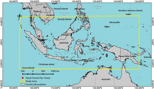
This study was conducted in a region of South East Asia centred on Indonesia and bounded by 94° to 154°E and 13°S to 13°N (Figure 1). In this region, there is one Flux Tower site located at Pasoh Forest Malaysia precisely at 102° E and 3°N that collects the daily NDVI observations from October 2008 to present.

Figure 1. Study area includes all of Indonesia and parts of other South East Asian countries.

Data

Coarse and moderate resolution NDVI data processed with different sampling time intervals and post-processing algorithms from the applications listed in Table 1 were retrieved from the respective online repositories. We aggregated weekly, tri-monthly and bi-monthly data into monthly data using a maximum value composites (MVC) analysis (Holben, 1986). In the case of data sampled weekly, weeks with data in 2 months were treated as follows: NDVI values at the start and end of the month were linearly interpolated using the last weekly values, and assuming that the weekly data represented the end of the week value, data were composited into monthly data by taking the maximum value. Further, post-processing was performed on all datasets (except for the AVHRR NESDIS and VIIRS NESDIS applications) using the adaptive Savitzky-Golay filter in Timesat (Jönsson & Eklundh, 2004) to minimize possible effects of atmospheric disturbances such as clouds and haze. A filter of adjacent data points was applied to smooth time series data to avoid massive change of the original values.

NDVI data from different satellite missions have different starting and ending dates, and also different temporal archives were selected to have the greatest number of datasets overlapping and the longest period of continuous data and statistical analysis of pairwise comparisons and trend analysis were performed. For pairwise comparison and trend analysis, the data period was divided into two sub-periods to permit analysis of newly released datasets such as Proba-V and VIIRS NESDIS and currently operating datasets such as AVHRR NESDIS, METOP, MODIS TERRA, MODIS AQUA, VIIRS NESDIS and PROBA V as follows: 1) April 2007 to March 2012 (60 months), and 2) January 2014 to December 2015 (24 months). In addition, pairwise assessments were performed for the period of November 2013 to May 2014 (7 months) to analyze the compatibility of SPOT VGT and PROBA-V.

There are three analyses conducted to compare and evaluate the similarity and performance of coarse NDVI products, such as 1) Pearson’s correlation, 2) trend and breakpoint analysis and 3) comparison with vegetation indices data from moderate spatial resolution data and flux tower data.

Pairwise comparison between NDVI products

The pairwise comparison was used to estimate the degree of differences between NDVI observations for overlapping observations. This analysis was performed using Pearson correlation at several spatial resolutions. We divided the analysis into resolution categories of 8, 4 and 1 km and resampled data collected at 1 and 4 km resolution using the bilinear method to obtain data in the coarsest resolutions of 4 and 8 km resolutions categories. Further zonal analysis using the land cover map using the type 3 classification scheme excluding the water category (Table 2) of MODIS land cover MCD12Q1 (Friedl et al., 2010) in 2013 was performed with an original spatial resolution of 500 m in order to understand the general agreement of correlation for different land cover categories.

Table 2. Type 3 classification scheme of MOD12Q1 and the associated notation for each classes in this study.

Category	Notation	Category	Notation
Grasses/Cereal crops	Grass/Cer	Deciduous Broadleaf Forests	Deciduous BF
Shrubs	Shrubs	Evergreen Needleleaf Forests	Evergreen NF
Broadleaf Crops	Broadleaf Cr	Deciduous Needleleaf Forests	Deciduous NF
Savanna	Savanna	Non-Vegetated	Non-Veg
Evergreen Broadleaf Forests	Evergreen BF	Urban	Urban

Trend and breakpoint analysis

Aside from performing a correlation analysis, we also performed a trend analysis to estimate the directional changes in NDVI time series to estimate whether different sensors produced the same trend over the same observation period. Trend analysis was performed using the Mann–Kendall test in Rstudio utilizing the Kendall package (McLeod, 2005) after de-seasonalizing NDVI time series data by subtracting the seasonal monthly means from the raw values over a same time periods (60 months from April 2007 to March 2012 and 24 months from Jan 2014 to December 2015). We used the Mann–Kendall test to estimate trends in time series data, including NDVI time series, because of its ability for detecting significant trends (Li et al., 2014), which are useful for comparing trend maps among different datasets.

Using the time series data, additional analysis to detect breakpoint or abrupt change from vegetation time series data can be performed. The breakpoints detected from vegetation indices including NDVI were identified to relate to the cover change (i.e. deforestation), and were also used for consistency assessment (Tian et al., 2015). In this study, the biggest point resembling the breakpoint with the biggest magnitude of change was detected by using bfast package in R (Verbesselt, Hyndman, Newnham, & Culvenor, 2010). Within the time periods, the month of breakpoints during 2007–2012 (5 years), and 2014–2015 (2 years) identified from different NDVI coarse resolution products were classified annually and compared one to another.

Besides comparing the annual breakpoint maps, we also compared trend maps and the annual breakpoints from different NDVI time series by reclassifying the type of trend based on slopes and p-values as shown in Table 3. From these categories, we calculated the percentage of area that was labelled with the same trend on different maps by graphing the trend distribution into a matrix as illustrated in Table 4.

Table 3. Trend map categories derived using the Mann–Kendall test.

Trend’s type	Slope (S)	P-value	Trend map categories
Significant negative	S < 0	p ≤ 0.05	SN
Non-significant negative		0.05 < p ≤ 0.1	NS
No trend with negative tendency		p > 0.1	NT
No trend with positive tendency	S > 0	p > 0.1
Non-significant positive		0.05 < p ≤ 0.1	NS
Significant positive		p ≤ 0.05	SP

Table 4. Matrix to calculate the percentage of similarity.

	Categories	Trend Map A
		SN	NS	NT	SP
Trend map	SN	A	B	C	D
	NS	E	F	G	H
	NT	I	J	K	L
	SP	M	N	O	P

From the matrix in the Table 3, we calculated the percentage of trend map by dividing the pixels that fall into the same categories in both maps divided by the total pixels as showed in the following equation 1:

where A, F, K and P denote the diagonal cells in Table 3 that hold the number of pixels that possess the same trend categories in both maps.

Regression analysis with Landsat data and in situ measurements

The ability of coarse resolution NDVI products when presenting NDVI values was compared with the two data sets: 1) Landsat systems (Landsat 5 TM and 8 OLI) and 2) flux tower measurements by constructing the ordinary least square (OLS) regression. This regression analysis was conducted as an alternative due to the lack of field measurements of vegetation biophysical features during the time periods in Indonesia needed to estimate the performance of coarse resolution NDVI products when estimating the biophysical properties. In addition, the comparison with the available global raster data of vegetation biophysical properties may create bias since those data were originated and constructed from the sensors of coarse NDVI products, for instance, LAI and fPAR estimated from MODIS, SPOT VGT and Proba V, and tree cover percentage from MODIS and AVHRR data (Baret et al., 2007; Defries, Hansen, Townshend, Janetos, & Loveland, 2000; DiMiceli et al., 2011; Myneni, Knyazikhin, & Park, 2015; Sánchez, Camacho, Lacaze, & Smets, 2015; Yang et al., 2006).

The assessment with moderate and detailed spatial resolution data were performed with the assumption that Landsat systems and flux tower data have greater quality when used to predict biophysical properties with their detailed spatial resolution of Landsat system and flux tower data, and complete spectral bands of Landsat systems. Landsat data were employed along with other detailed resolution data as one of the input data to model fraction cover estimated from MODIS and also often used to create detailed resolution LAI map from ground sampling data to validate the coarse data estimation of vegetation biophysical properties (Chen et al., 2002; Defries et al., 2000; Fernandes, Butson, Leblanc, & Latifovic, 2003; Kang et al., 2016; Wang et al., 2004; Yang et al., 2007).

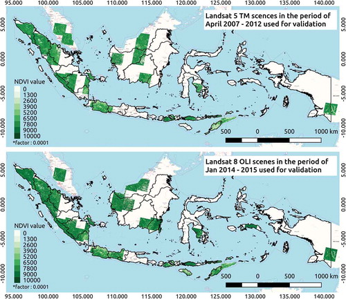
Landsat data and coarse resolution satellite imageries have a different temporal resolution or revisit time. The pixel values from Landsat system were recorded in every 16 days, while NDVI from coarse resolution products were constructed from daily, weekly, 10-day or bi-monthly data. To minimize the bias due to the difference in the revisit time, the analysis was conducted by comparing the average values from the minimum three continuous cloud-masked Landsat data with the average values of NDVI from coarse products at the same periods to generate the OLS regression line. We collected 46 scenes of time series data originated from 255 individual scenes of Landsat 5 TM during 2007–2012, and 73 scenes of time series data originated from 472 scenes of Landsat 8 OLI during 2014–2015 (Figure 2). Both Landsat systems data obtained at Level-2 correction, which pixel values represent at-surface reflectance and were resampled to 8-km.

Figure 2. Distribution of average NDVI values from time series Landsat 5 TM and 8 OLI used for validating NDVI from coarse resolution data.

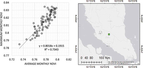
Besides using Landsat as comparison, we also measured the RMSE of NDVI calculated from satellite observations with measurements taken at the flux tower located in the Pasoh Tropical Rainforest, Malaysia (Figure 3). At the flux tower, NDVI measurements have been taken every 30 min on days with no rain since October 2008 along with monitoring of other environmental parameters (details on homepage: http://www.bluemoon.kais.kyoto-u.ac.jp/pasoh/main.html) (Nakaji et al., 2014). The data enabled us to compare NDVI values collected at the flux tower with the values collected in satellite data over the period of overlapping data collection. The monthly flux tower data were analyzed by taking the average monthly values and the maximum monthly values (Figure 3) and comparing them to the MVC data of NDVI measurement. Statistical analysis was performed by deriving the root mean square error (RMSE) and R² values for the comparison between observed values from satellites observation and actual values from the flux tower measurement.

Figure 3. Scatter plot of monthly average and maximum NDVI values at Pasoh Rainforest, Malaysia.

In summary, the OLS regression was performed by using NDVI data as listed in Table 5. The regression analysis was performed by using 1) all pixels in the imageries, 2) vegetation pixels only, and, 3) major vegetation biomes such as a) evergreen broadleaf forests (EBF), b) savanna (SAV), and c) cropland (CRO) to assess the performance of the VI values of coarse resolution products in different vegetation cover types.

Table 5. NDVI data used in the regression analysis.

Data	Time range	Original data observation	Processing	Number of data
Landsat 5 TM	April 2007–March 2012	16 days	1.) Averaging the pixel values of more than 3 Landsat imageries with continuous time acquisition within the time range and 2.) resampling to 8-km (2007–2013) and 4-km (2014–2015)	255 scenes averaged into 46 imageries
Landsat 8 OLI	January 2014–December 2015			472 scenes averaged into 73 imageries
Flux Tower data	October 2008–2015	30-minutes data during the non-rainy day	Averaging the 30 min data to represent monthly data	1.) 40 months (2008–2012), and 2.) 24 months (2014–2015)

Results and discussion

Pairwise correlation between NDVI datasets

Pairwise analysis of NDVI datasets collected by different satellites and prepared for comparison in the 7, 24 and 60 months periods in the spatial resolution categories of 1, 4 and 8 km had Pearson correlation coefficients that were positive but ranged from weak to moderate (Table 6). For 1 km spatial resolution, the strongest coefficient (0.52) was obtained for the comparison of METOP and Proba during the observation period 2014–2015, followed by the pairwise comparison of METOP and SPOT with a coefficient of 0.50. On the other hand, the weakest coefficient (0.17) was obtained for the comparison of Terra and AQUA in 2014–2015, and this value was smaller than in the first analysis in 2007–2012 when it was 0.35. PROBA-V and SPOT showed a relatively strong correlation coefficient (0.44) for datasets at the original spatial resolution. At a spatial resolution of 4 km, AVHRR NESDIS and VIIRS NESDIS showed a strong correlation with 0.67 while the comparison of PROBA-V and METOP was the second strongest with 0.54. The weakest correlation coefficient (0.27) at this spatial resolution was for the comparison of MERIS and AQUA. This combination indicates that extended measurement to expand NDVI observation is feasibly achieved by combining AVHRR NESDIS with VIIRS NESDIS. At 8 km spatial resolution, METOP and SPOT combination followed by SPOT and TERRA combination became the two strongest correlations with 0.63 and 0.58, respectively. In addition, the longest NDVI observation from different sensors can be generated by combining the AVHRR-based NDVI products from GIMMS3G data and NESDIS due to the strong correlation between those datasets with 0.42 (correlation of coefficient).

Table 6. Correlation coefficients for pairwise comparison of different NDVI datasets at spatial resolutions of 1, 4 and 8 km during April 2007 to March 2012 (60 months) and January 2014 to December 2015 (24 months).

Pixel Size	Period	April 2007–Dec 2012							Jan 2014–Dec 2015
	Data	MA	MRS	MTP	MT	SV			Data	MA	MTP	PV	MTP
1 km	MA	100							MA	100
	MRS	36.64	100						MTP	35.19	100
	MTP	36.05	36.01	100					PV	36.05	37.98	100
	MT	39.96	36.68	37.44	100				MT	35.81	34.94	35.92	100
	SV	36.21	34.71	40.94	38.52	100
	Data	MA	MRS	MTP	MT	SV	AN		Data	AN	VN	MA	MTP	PV	MT
4 km	MA	100							AN	100
	MRS	37.77	100						VN	38.23	100
	MTP	36.62	35.61	100					MA	34.84	36.13	100
	MT	42.88	35.62	39.25	100				MTP	35.52	35.74	35.22	100
	SV	37.49	36.42	44.12	42.25	100			PV	35.99	37.31	37.42	40.25	100
	AN	37.04	34.76	36.05	36.26	36.17	100		MT	33.37	34.75	38.04	35.37	38.01	100
	Data	GM	MA	MRS	MTP	AN	MT	SV	Legend
8 km	GM	100							GM : GIMMS3G			AN : AVHRR NESDIS
	MA	37.45	100						PV : PROBA V			VN : VIIRS NESDIS
	MRS	35.12	38.05	100					MRS : MERIS			MT : MODIS TERRA
	MTP	34.23	36.06	35.30	100				MTP : METOP			MA : MODIS AQUA
	AN	35.31	37.84	35.12	35.90	100			SV : SPOT VGT
	MT	36.10	42.99	38.71	39.59	37.08	100			Data with relatively low percentage
	SV	33.13	36.56	36.30	46.44	36.89	42.30	100

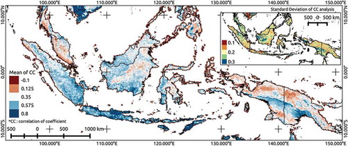
The average correlation of coefficient map, as shown in the Figure 4, was estimated by resampling the 61 correlation of coefficient combination in the previous analyses into 8 km and compiling the average and standard deviation values from that pairwise combination. The map indicated the distribution of strong and weak values within specific categories. To investigate whether that distribution corresponds to specific land cover classes, we performed the zonal analysis using the land cover categories.

Figure 4. Average correlation of coefficient map of NDVI products estimated from the pairwise comparison between existing NDVI products.

Variation of correlation coefficients across land cover types

Mapping pairwise comparison correlation coefficients by land cover type in a zonal analysis at a spatial resolution of 1, 4 and 8 km revealed that some land cover types showed consistently strong or weak correlation coefficients at different spatial resolutions as showed in the Figure 5. On the correlation coefficient maps for spatial resolution of 1 km, there was a strong agreement for grass/cereal crops, broadleaf crops and SAV with average correlation coefficients of 0.67, 0.66 and 0.63, respectively, whereas correlation coefficients showed weak agreement for EBF, evergreen needleleaf forest and non-vegetated classes with 0.32, 0.26 and 0.34, respectively. At 4 km spatial resolution, great agreement (strong average correlation coefficient) was found in the classes of broadleaf crops and SAV with 0.84 and 0.76, respectively, and a moderate agreement was found for grassland/cereal crops (0.68). The land cover types EBF, evergreen needleleaf forest and non-vegetated class showed weak correlation coefficients at the spatial resolution of 4 km and had average values of 0.42, 0.37 and 0.41, respectively, at 8 km spatial resolution. Likewise, broadleaf crops, SAV and grass/cereal crops showed strong correlation coefficients of 0.81, 0.73 and 0.63, respectively, at 8 km spatial resolution.

Figure 5. Boxplot showing the statistical properties of correlation coefficient for different land cover types at different spatial resolutions of 1, 4 and 8 km.

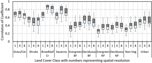
Based on correlation coefficient results, strong correlation values for SAV and grassland land cover types which have frequent vegetation cover change are mainly influenced by climatic factors when the distinct pattern of precipitation and temperatures appeared in the dry and wet season. Agreement between the phenology and climate parameters is strong for these land cover types due to the dependence of the growth of those land cover types to the water availability which differs at different seasons (dry and wet), while vegetation cover types such as evergreen broad/needleleaf forest are less influenced by climate variables, and the values are stable but different, thus producing weak average correlation coefficients. The weak agreement in those land cover types corroborates the research of Rasmus Fensholt and Proud (2012), which found great differences in trends in land cover types of needleleaf forest and broadleaf forest.

Trend and breakpoint analysis

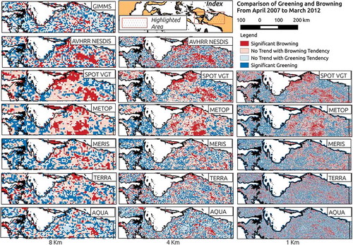
Trend analysis using the Mann–Kendall test generated Kendall’s slope map with corresponding p-values. Mapping the associated p-values produces a spatial distribution showing areas with greening and browning trends that are statistically significant (p-value < 0.05) and areas with no significant trend for each NDVI application for the 60-month dataset (Figure 6). Pairwise comparison of trend results from different NDVI applications in terms of spatial agreement expressed as a percentage of the same or similar class producing maps that show agreement are shown in Table 7. The average spatial agreement between trend maps of different NDVI applications from different sensors and spatial resolutions was weak at 37.2 ± 2.5%.

Table 7. Percentage of spatial similarities in trend maps in vegetation areas estimated from different NDVI time series applications at spatial resolution of 1, 4 and 8 km.

	Period	April 2007–Dec 2012							Jan 2014–Dec 2015
Pixel Size	Data	MA	MRS	MTP	MT	SV			Data	MA	MTP	PV	MTP
1 km	MA	100							MA	100
	MRS	36.64	100						MTP	35.19	100
	MTP	36.05	36.01	100					PV	36.05	37.98	100
	MT	39.96	36.68	37.44	100				MT	35.81	34.94	35.92	100
	SV	36.21	34.71	40.94	38.52	100
	Data	MA	MRS	MTP	MT	SV	AN		Data	AN	VN	MA	MTP	PV	MT
4 km	MA	100							AN	100
	MRS	37.77	100						VN	38.23	100
	MTP	36.62	35.61	100					MA	34.84	36.13	100
	MT	42.88	35.62	39.25	100				MTP	35.52	35.74	35.22	100
	SV	37.49	36.42	44.12	42.25	100			PV	35.99	37.31	37.42	40.25	100
	AN	37.04	34.76	36.05	36.26	36.17	100		MT	33.37	34.75	38.04	35.37	38.01	100
	Data	GM	MA	MRS	MTP	AN	MT	SV	Legend
8 km	GM	100							GM : GIMMS3G			AN : AVHRR NESDIS
	MA	37.45	100						PV : PROBA V			VN : VIIRS NESDIS
	MRS	35.12	38.05	100					MRS : MERIS			MT : MODIS TERRA
	MTP	34.23	36.06	35.30	100				MTP : METOP			MA : MODIS AQUA
	AN	35.31	37.84	35.12	35.90	100			SV : SPOT VGT
	MT	36.10	42.99	38.71	39.59	37.08	100			Data with generally smaller percentages
	SV	33.13	36.56	36.30	46.44	36.89	42.30	100

Figure 6. Greening and browning trends over 60 months mapped using different NDVI time series applications at different spatial resolutions.

In 8 km NDVI data, agreement varied from 33.13% (GIMMS vs. SPOT VGT) to 46.44% (Metop vs. SPOT VGT). The spatial agreement with GIMMS3G data on the trend map was relatively weak with only 35.2% on average, with the strongest agreement for the comparison of MODIS Aqua with GIMMS data (37.45%). In 4 km spatial resolution analysis, a strong agreement was observed between SPOT VGT and Metop (44.12%) and between Aqua and Terra (42.88%). Data assessed over the period from April 2007 to March 2012 revealed that the strongest agreement by using AVHRR NESDIS was shown with Aqua (37.04%), although other datasets showed more or less similar level of agreement. In the assessment for the second period (January 2013 to December 2014), which involved the VIIRS datasets and Proba-V, AVHRR NESDIS had the greatest agreement with VIIRS NESDIS (38.23%), while the second strong agreement was obtained from the pairwise comparison of Metop and Proba-V (40.25%).

The trend map assessed for the original spatial resolution scale of 1 km revealed the strongest agreement between trend maps with an average of 37.32% (Apr 2007 to Mar 2012) and 35.98% (Jan 2013 to Dec 2014). The strongest agreement was obtained from METOP and SPOT VGT with 40.94% of similarity percentage. In the period of January 2014 to December 2015, the trend map from Proba-V showed slightly smaller agreement with another trend map from other datasets in this assessment, the strongest agreement was observed with the Metop data (37.98%).

This analysis also revealed the possibility of producing contradictory results in trend maps estimated from different satellite observation, such as achieving significantly negative trends in one trend map but significantly positive trends in another trend map. By taking the average of the matrix of similarity tables and measuring the distribution of contradictory category results from 16, 30 and 21 combinations of trend maps at 1, 4 and 8 km spatial resolution scales, respectively, we found a small percentage of significant contradictory trends from SN to SP (around 2.5–5.39%) as shown in Table 8. The percentage of contradictory trends seems small if we look at the proportion from the total; however, this percentage of contradictory trends may account for a 10–23% portion of detected significant greening or browning (SP and SN). In conclusion, there was approximately 0.20–0.25 (20–25%) possibility that a trend detected as being significant from one NDVI observation might be classified as a significant opposite trend if another NDVI observation was used.

Table 8. Matrix of average distribution of spatial similarities in vegetation areas from trend maps derived using different NDVI applications.

	Categories	SP	SN	NS	NT
1 k	SP	6.21 ± 3.6	2.65 ± 1.3	1.25 ± 0.4	5.31 ± 1.8
	SN	8.2 ± 3.1	12.46 ± 2.5	3.95 ± 0.3	19.86 ± 0.8
	NS	1.76 ± 0.6	2.42 ± 0.7	0.79 ± 0.1	3.76 ± 0.4
	NT	4.72 ± 1.9	9.96 ± 2.1	2.76 ± 0.5	13.94 ± 1.6
4 km	SP	6.88 ± 4	3.06 ± 1.9	1.46 ± 0.6	6.04 ± 2.7
	SN	7.9 ± 3.1	12.58 ± 2.5	3.96 ± 0.3	19.75 ± 1
	NS	1.78 ± 0.6	2.51 ± 0.7	0.81 ± 0.1	3.78 ± 0.4
	NT	3.98 ± 1.8	9.79 ± 2.5	2.6 ± 0.5	13.11 ± 2
8 km	SP	8.89 ± 4.1	2.19 ± 1.5	1.43 ± 0.6	5.53 ± 2.5
	SN	10.28 ± 3.5	11.04 ± 2.7	3.89 ± 0.3	19.85 ± 1.5
	NS	2.18 ± 0.7	1.92 ± 0.5	0.72 ± 0	3.51 ± 0.3
	NT	5.09 ± 2.3	8 ± 1.7	2.4 ± 0.4	13.09 ± 1.7
		: percentage of same trends at both trend maps
		: percentage of contrasting significant trends

The similar discrepancy among the coarse resolution NDVI products also appeared in the trend map analysis. In the first analysis to detect annual breakpoints during 2007 – 2012 (Table 9a), the similarity percentages were fallen between 29.12 and 40.51%. The greatest level of similarity percentage when identifying breakpoint was achieved by using SPOT VGT and MODIS Terra with 40.51% of similarity, while the smallest came from comparing STAR NESDIS with AVHRR GIMMS. In the period of 2014–2015 (Table 9b), the percentages were much bigger considering that there were only two categories of 2014 and 2015 for the detected breakpoints. The similar percentages fell within the range of 51.1– 58.42%. The greatest similarity percentage in this period was produced by comparing STAR VIIRS and NESDIS data with 58.42%, while the weakest came from comparing STAR NESDIS with MODIS TERRA data.

Table 9. Similarity percentages of breakpoints detected from coarse resolution NDVI products during a) 2007–2012, and b) 2014–2015.

a) April 2007–Dec 2012								b) Jan 2014–Dec 2015
Data	GM	MA	MRS	MTP	AN	MT	SV	Data	MA	MTP	PV	MT	VN	AN
GM	100							MA	100
MA	29.58	100						MTP	57.50	100
MRS	29.63	32.35	100					PV	56.62	57.98	100
MTP	29.30	32.87	33.74	100				MT	55.13	55.21	55.87	100
AN	29.12	34.14	32.19	32.29	100			VN	52.54	54.12	53.65	52.20	100
MT	29.72	37.97	34.86	35.25	34.22	100		AN	51.32	51.70	52.12	51.10	58.42	100
SV	29.30	35.74	35.63	38.66	35.66	40.53	100		Data with relatively smaller percentages

Comparisons with Landsat and flux tower measurements

The comparison between NDVI from coarse resolution products and Landsat data revealed different level R² from 0.19 (VIIRS) to 0.64 (SPOT VGT and PROBA-V). Further removal of non-vegetation pixel data from the regression analysis still put SPOT VGT and PROBA-V with the data that have strong relationships with Landsat with the R² of 0.68 (SPOT VGT) and 0.67 (PROBA-V), respectively (Figure 7). In addition, MODIS-Terra and METOP were the third and fourth strongest with 0.54 and 0.53 when all pixels were considered, while MODIS-Terra and Aqua were the third and fourth strongest with 0.58 and 0.53 when only vegetated pixels were included in the regression analysis. The complete regression models from all coarse products can be seen in the Supplementary Materials 1 and 2 (S1). This analysis concluded that the newer products such as SPOT VGT, Proba-V, MODIS-Terra, Metop and Aqua matched strongly with the Landsat data compared than the AVHRR-based NDVI index (i.e. GIMMS or NESDIS).

Figure 7. NDVI values for the vegetation cover taken from a.) SPOT-VGT (during 2007 – 2012) and b.) MODIS Terra (during 2014 – 2015) displayed a strong fit with NDVI from Landsat 5 TM and Landsat 8 OLI.

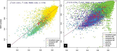
The regression in specific vegetation cover types revealed that generally MODIS Terra/Aqua, SPOT VGT, Proba-V and METOP generated stronger model fit in different vegetation cover types. Generally, weakest linear fit can be found when modelling the EBF class with the maximum 34% of variance in EBF can be explained by using SPOT VGT data. In modelling SAV class, overall greater linear fits were displayed from NDVI coarse products with the range of 31% (GIMMS3g) to 76% (SPOT VGT) of the explained variance. Overall strong fit also can be found in modelling CRO class with the exception from GIMMS3g v0 data that only able to explain 5% of the variance. The regression results and the corresponding RMSE values can be discovered at Table 10.

Table 10. Regression results from NDVI coarse resolution products versus Landsat systems.

a) Regression with Landsat 5 TM during 2007–2012 in 8-km pixel size
Category	GIMMS			Modis Terra			Modis Aqua			SPOT VGT			METOP			MERIS			NESDIS
	RMSE	r2	n	RMSE	r2	n	RMSE	r2	n	RMSE	r2	n	RMSE	r2	n	RMSE	r2	n	RMSE	r2	n
All pixels	0.12	0.35	13,055	0.1	0.54	13,055	0.1	0.52	13,055	0.09	0.64	13,055	0.1	0.53	13,055	0.11	0.45	13,055	0.12	0.31	5710
Veg. only pixels	0.09	0.32	11,747	0.07	0.58	11,745	0.07	0.53	11,746	0.06	0.68	11,746	0.08	0.51	11,746	0.09	0.34	11,746	0.12	0.28	5181
CRO	0.07	0.05	215	0.05	0.61	214	0.05	0.55	216	0.05	0.59	216	0.05	0.52	216	0.06	0.43	216	0.05	0.46	48
SAV	0.12	0.31	1642	0.1	0.54	1638	0.11	0.48	1638	0.07	0.76	1640	0.1	0.53	1639	0.11	0.4	1640	0.1	0.6	1430
EBF	0.06	0.09	9693	0.05	0.25	9696	0.06	0.18	9695	0.05	0.34	9692	0.05	0.25	9693	0.06	0.11	9692	0.06	0.01	3644
b) regression with Landsat 8 OLI during 2014–2015 in 4-km pixel size
	Modis Terra			Modis Aqua			METOP			Proba-V			VIIRS			NESDIS
Category	RMSE	r2	n	RMSE	r2	n	RMSE	r2	n	RMSE	r2	n	RMSE	r2	n	RMSE	r2	n
All pixels	0.12	0.59	56,566	0.13	0.55	56,566	0.13	0.54	56,551	0.11	0.64	59,127	0.15	0.19	51,330	0.13	0.1	45,305
Veg. only pixels	0.07	0.67	46,999	0.09	0.54	47,012	0.09	0.49	47,010	0.07	0.67	49,582	0.11	0.2	44,409	0.12	0.06	43,047
CRO	0.06	0.71	1271	0.07	0.65	1272	0.07	0.62	1276	0.07	0.67	1271	0.09	0.44	1259	0.09	0.33	1245
SAV	0.07	0.62	10,859	0.07	0.59	10,865	0.09	0.45	10,859	0.07	0.6	10,877	0.09	0.46	10,740	0.09	0.35	10,520
EBF	0.06	0.26	32,830	0.07	0.11	32,841	0.06	0.2	32,836	0.06	0.31	35,400	0.07	0.01	30,382	0.08	0	29,267

Further analysis was conducted between NDVI data collected at the flux tower in Pasoh Forest, Malaysia with the pixel value of NDVI from satellite data in the same coordinate where the Flux Tower is located for monthly averages, and the comparison was evaluated in terms of RMSE and R² values (Table 11). GIMMS3G ver. 0, SPOT VGT, METOP, MODIS TERRA, MODIS AQUA and PROBA V showed comparable average RMSE with a range of 0.06 to 0.09 with SPOT VGT being the greatest and Proba V being the smallest, and the maximum RMSE for these data was 0.04 to 0.11 with the same pattern of results. On the other hand, a significant difference from flux tower measurements was observed for AVHRR NESDIS and VIIRS NESDIS, which showed similar average RMSE (0.41 and 0.16, respectively) and maximum RMSE (0.44 and 0.2, respectively), which differed from comparison results for the other NDVI applications. Weak R² values in this analysis indicate a weak correlation between data collected at the flux tower and satellite data used in this study. Although a weak R² value might be due to the density of the canopy, NDVI applications were most likely saturated in the area of the flux tower, which also results in smaller R² values. The density of canopy cover in this area was reflected in the comparison of NDVI values from the flux tower datasets and satellites with the RMSE of the average and maximum values being not markedly different, indicating constant and stable NDVI values in this area.

Table 11. Linear regression and corresponding R-squared and RMSE derived from comparison between NDVI values from satellite data and flux tower datasets.

Data (n)	Regression (average)	R^2	RMSE	Regression (max)	R^2	RMSE
GIMMS3G Ver.0 (40)	Y = 0.81–0.03x	0.02	0.06	Y = 0.83–0.02x	0.01	0.06
AVHRR NESDIS (40)	Y = 0.8–0.05x	0.03	0.41	Y = 0.81 + 0.01x	0	0.44
AVHRR VIIRS (24)	Y = 0.69 + 0.13x	0.18	0.16	Y = 0.76 + 0.08x	0.08	0.2
SPOT VGT (40)	Y = 0.85–0.08x	0.03	0.06	Y = 0.9–0.1x	0.08	0.04
METOP (40)	Y = 0.75 + 0.04x	0.02	0.07	Y = 0.81 + 0.01x	0	0.05
MERIS (40)	Y = 0.76 + 0.02x	0.01	0.01	Y = 0.82–0.01x	0	0.01
MODIS TERRA (40)	Y = 0.84–0.07x	0.03	0.07	Y = 0.87–0.06x	0.04	0.04
MODIS AQUA (40)	Y = 0.79–0.01x	0	0.09	Y = 0.9–0.1x	0.06	0.05
PROBA V (24)	Y = 0.8–0.04x	0.05	0.11	Y = 0.84–0.04x	0.04	0.1

Comparing pixel and point measurements from the flux tower observations was apparently not a proper comparison since satellite values were influenced by the surrounding environment and were more likely to be exposed to atmospheric disturbances than the flux tower measurements. In addition, observations from more than one site in different areas should be used to estimate the RMSE. However, for this analysis, most of the error deviation for all NDVI applications appears to be relatively similar, with the exception in AVHRR NESDIS and VIIRS NESDIS, which somehow have much bigger RMSE.

Discussion

The comparison analysis in this study, which comprises of three sub-analyses of correlation coefficients, trend and breakpoint analysis using the Mann–Kendall test, and bfast package, and comparison of satellite data with NDVI from Landsat and flux tower, showed the variability in NDVI values and their consistencies in trends, and performance over South East Asia landscape. The correlation coefficients from the measurement of different NDVI time series products showed weak to medium strength with AVHRR GIMMS, and monthly STAR NESDIS had an overall smaller correlation with other datasets. In order to ensure seamless integration of multiple datasets including inter-sensor NDVI time series observations, especially in areas covered by broadleaf or needleleaf forest which were common to be found in this area, appropriate pre-processing algorithms to address factors that affect NDVI values are needed. It is also worth noting the possibility of performing calibrations between different NDVI time series products, particularly in this region of South East Asia, and these should be performed using values in climate-dependent vegetation types such as SAV, broadleaf crops and grassland areas.

The variability of NDVI values between different NDVI products as shown in the pairwise comparisons with weak to medium correlation coefficients also gets reflected in the trend and breakpoint map similarity analysis, which exhibits a similar weak to medium percentage of a similar trend with AVHRR GIMMS and STAR NESDIS data became the data with smaller overall similarity. The possibility of smaller paired similarity between STAR NESDIS and STAR VIIRS can be caused by the aggregation process from 7-day data into monthly data.

The comparison of coarse resolution NDVI products and Landsat data depicted that some sensors such as SPOT VGT, PROBA V and MODIS Terra/Aqua had an overall strong relationship when linked with Landsat data with overall strong linear in representing the values of different vegetation cover types. On the contrary, weaker relationships were showed by GIMMS, NESDIS and VIIRS data. It should be noted that at the time of conducting this study, the newer version of AVHRR GIMMS ver.1 was launched which may have an improvement over the GIMMS ver.0 data that was used in this study.

The performance of coarse resolution NDVI data in the dense canopy forest as represented by the flux tower data showed that different NDVI time series observations have similar RMSE when compared to NDVI datasets at the flux tower in the forest area. The correlation coefficient was quite weak as NDVI tended to become saturated in the area where the comparison was undertaken. Furthermore, this assessment comparing flux tower measurements is not sufficient to make a conclusion on the overall quality of NDVI time series products since data from only a single site of flux tower was used. In addition, linking the time series values of NDVI with the actual field datasets is also essential to assess the performance of this index when used to model vegetation biophysical properties and to understand what kind of properties in vegetation being represented by this vegetation index.

Conclusion

This study emphasized the discrepancies among the available and existing NDVI products and stressed the importance of fully understanding the limitation and possible differences in outputs that might be present, especially when time series analysis is performed using a single dataset. Other researchers aiming to use the coarse data to estimate the trends from NDVI are suggested to employ multiple satellite time series observations to confirm conclusions and to identify methods for reconciling discordant findings by various NDVI applications. Furthermore, a vegetation index that possesses the smaller sensitivity to the atmospheric gasses compositions and background variations is beneficial to generate stable and comparable vegetation index products (Huete et al., 2002). Therefore, another effort can be made by contrasting time series analysis using NDVI with other proxy parameters that are less impacted by atmospheric disturbances; such as vegetation optical depth (VOD) or Enhanced Vegetation Index (EVI), which does not saturate in areas of dense vegetation. In future studies, assessing the quality of remote-sensing-based vegetation proxy by linking the values with the ground datasets is essential to further understand the performance of vegetation indices when used to model the vegetation biophysical properties.

Geolocation Information

The study area is located at 94° to 154°E and 13°S to 13°N.

Acknowledgments

The authors would like to express their appreciation to the managers of the databases for making data freely available, Assoc. Prof. Tatsuro Nakaji from Hokkaido University, and Prof. Yoshiko Kosugi from Kyoto University for providing access to the flux tower data in Pasoh Forest, Malaysia, Forest Research Institute Malaysia (FRIM) for managing the study site`s data and Monbukagakusho (MEXT) for providing scholarships to the first author for this research.

Disclosure statement

No potential conflict of interest was reported by the authors.

References

- Alcaraz-Segura, D., Liras, E., Tabik, S., Paruelo, J., & Cabello, J. (2010). Evaluating the consistency of the 1982–1999 NDVI trends in the Iberian Peninsula across four time-series derived from the AVHRR sensor: LTDR, GIMMS, FASIR, and PAL-II. Sensors, 10(2), 1291–1314.
- Baldi, G., Nosetto, M.D., Aragón, R., Aversa, F., Paruelo, J.M., & Jobbágy, E.G. (2008). Long-term satellite NDVI data sets: Evaluating their ability to detect ecosystem functional changes in South America. Sensors, 8(9), 5397–5425.
- Baret, F., & Guyot, G. (1991). Potentials and limits of vegetation indices for LAI and APAR assessment. Remote Sensing of Environment, 35(2), 161–173.
- Baret, F., Hagolle, O., Geiger, B., Bicheron, P., Miras, B., Huc, M., … Samain, O. (2007). LAI, fAPAR and fCover CYCLOPES global products derived from VEGETATION: Part 1: Principles of the algorithm. Remote Sensing of Environment, 110(3), 275–286.
- Brown, M.E., Pinzón, J.E., Didan, K., Morisette, J.T., & Tucker, C.J. (2006). Evaluation of the consistency of long-term NDVI time series derived from AVHRR, SPOT-vegetation, SeaWiFS, MODIS, and Landsat ETM+ sensors. IEEE Transactions on Geoscience and Remote Sensing, 44(7), 1787–1793.
- Carlson, T.N., & Ripley, D.A. (1997). On the relation between NDVI, fractional vegetation cover, and leaf area index. Remote Sensing of Environment, 62(3), 241–252.
- Chen, J.M., Pavlic, G., Brown, L., Cihlar, J., Leblanc, S., White, H., … Trofymow, J. (2002). Derivation and validation of Canada-wide coarse-resolution leaf area index maps using high-resolution satellite imagery and ground measurements. Remote Sensing of Environment, 80(1), 165–184.
- Cong, N., Wang, T., Nan, H., Ma, Y., Wang, X., Myneni, R.B., & Piao, S. (2013). Changes in satellite-derived spring vegetation green-up date and its linkage to climate in China from 1982 to 2010: A multimethod analysis. Global Change Biology, 19(3), 881–891.
- Defries, R.S., Hansen, M.C., Townshend, J.R., Janetos, A., & Loveland, T. (2000). A new global 1‐km dataset of percentage tree cover derived from remote sensing. Global Change Biology, 6(2), 247–254.
- Defries, R.S., & Townshend, J.R.G. (1994). NDVI-derived land cover classifications at a global scale. International Journal of Remote Sensing, 15(17), 3567–3586.
- Detsch, F., Otte, I., Appelhans, T., & Nauss, T. (2016). A comparative study of cross-product NDVI dynamics in the Kilimanjaro region-a matter of sensor, degradation calibration, and significance. Remote Sensing, 8(2). doi:10.3390/rs8020159
- Didan, K., Munoz, A.B., & Huete, A. (2015). Modis vegetation index user’s guide (MOD13 Series) 2015(June). The University of Arizona,Publisher name: Vegetation Index and Phenology Lab.
- DiMiceli, C., Carroll, M., Sohlberg, R., Huang, C., Hansen, M., & Townshend, J. (2011). Annual global automated MODIS vegetation continuous fields (MOD44B) at 250 m spatial resolution for data years beginning day 65, 2000–2010, collection 5 percent tree cover. College Park, MD, USA: University of Maryland.
- Epiphanio, J.N., & Huete, A.R. (1995). Dependence of NDVI and SAVI on sun/sensor geometry and its effect on fAPAR relationships in Alfalfa. Remote Sensing of Environment, 51(3), 351–360.
- Erasmi, S., Propastin, P., Kappas, M., & Panferov, O. (2009). Spatial patterns of NDVI variation over Indonesia and their relationship to ENSO warm events during the period 1982–2006. Journal of Climate, 22(24), 6612–6623.
- Fensholt, R., Langanke, T., Rasmussen, K., Reenberg, A., Prince, S.D., Tucker, C., … Wessels, K. (2012). Greenness in semi-arid areas across the globe 1981–2007 — An earth observing satellite based analysis of trends and drivers. Remote Sensing of Environment, 121, 144–158.
- Fensholt, R., & Proud, S.R. (2012). Evaluation of earth observation based global long term vegetation trends — Comparing GIMMS and MODIS global NDVI time series. Remote Sensing of Environment, 119, 131–147.
- Fensholt, R., Rasmussen, K., Nielsen, T.T., & Mbow, C. (2009). Evaluation of earth observation based long term vegetation trends — Intercomparing NDVI time series trend analysis consistency of Sahel from AVHRR GIMMS, Terra MODIS and SPOT VGT data. Remote Sensing of Environment, 113(9), 1886–1898.
- Fensholt, R., Sandholt, I., & Stisen, S. (2006). Evaluating MODIS, MERIS, and VEGETATION vegetation indices using in situ measurements in a semiarid environment. IEEE Transactions on Geoscience and Remote Sensing, 44(7), 1774–1786.
- Fernandes, R., Butson, C., Leblanc, S., & Latifovic, R. (2003). Landsat-5 TM and Landsat-7 ETM+ based accuracy assessment of leaf area index products for Canada derived from SPOT-4 VEGETATION data. Canadian Journal of Remote Sensing, 29(2), 241–258.
- Friedl, M.A., Sulla-Menashe, D., Tan, B., Schneider, A., Ramankutty, N., Sibley, A., & Huang, X. (2010). MODIS Collection 5 global land cover: Algorithm refinements and characterization of new datasets. Remote Sensing of Environment, 114(1), 168–182.
- Gutman, G., Csiszar, I., & Romanov, P. (2000). Using NOAA/AVHRR products to monitor El Niño impacts: Focus on Indonesia in 1997–98. Bulletin of the American Meteorological Society, 81(6), 1189–1205.
- Holben, B. (1986). Characteristics of Maximum-Value Composite Images from Temporal AVHRR Data. International Journal of Remote Sensing, 7 (11). 1417–1434. doi:10.1080/01431168608948945
- Huete, A., Didan, K., Miura, T., Rodriguez, E.P., Gao, X., & Ferreira, L.G. (2002). Overview of the radiometric and biophysical performance of the MODIS vegetation indices. Remote Sensing of Environment, 83, 195–213.
- Jönsson, P., & Eklundh, L. (2004). TIMESAT - A program for analyzing time-series of satellite sensor data. Computers and Geosciences, 30(8), 833–845.
- Kang, Y., Özdoğan, M., Zipper, S.C., Román, M.O., Walker, J., Hong, S.Y., … Alonso, L. (2016). How universal is the relationship between remotely sensed vegetation indices and crop leaf area index? A global assessment. Remote Sensing, 8(7), 597.
- Kogan, F.N. (2001). Operational space technology for global vegetation assessment. Bulletin of the American Meteorological Society, 82(9), 1949–1964.
- Li, C., Qi, J., Yang, L., Wang, S., Yang, W., Zhu, G., … Zhang, F. (2014). Regional vegetation dynamics and its response to climate change—A case study in the Tao River Basin in Northwestern China. Environmental Research Letters, 9(12), 125003–125004.
- McLeod, A.I. (2005). Kendall rank correlation and Mann-Kendall trend test. R Package Kendall.
- Morton, D.C., Nagol, J., Carabajal, C.C., Rosette, J., Palace, M., Cook, B.D., … North, P.R.J. (2014). Amazon forests maintain consistent canopy structure and greenness during the dry season. Nature, 506(7487), 221–224.
- Myneni, R., Knyazikhin, Y., & Park, T. (2015). MOD15A2H MODIS/terra leaf area index/FPAR 8-day L4 global 500 m SIN grid V006. NASA EOSDIS Land Processes DAAC.
- Myneni, R.B., & Williams, D.L. (1994). On the relationship between FAPAR and NDVI. Remote Sensing of Environment, 49(3), 200–211.
- Nagol, J., Vermote, E., & Prince, S. (2014). Quantification of impact of orbital drift on inter-annual trends in AVHRR NDVI data. Remote Sensing, 6(7), 6680–6687.
- Nakaji, T., Kosugi, Y., Takanashi, S., Niiyama, K., Noguchi, S., Tani, M., … Kassim, A.R. (2014). Estimation of light-use efficiency through a combinational use of the photochemical reflectance index and vapor pressure deficit in an evergreen tropical rainforest at Pasoh, Peninsular Malaysia. Remote Sensing of Environment, 150, 82–92.
- Pettorelli, N., Vik, J.O., Mysterud, A., Gaillard, J.-M., Tucker, C.J., & Stenseth, N.C. (2005). Using the satellite-derived NDVI to assess ecological responses to environmental change. Trends in Ecology & Evolution, 20(9), 503–510.
- Pinzon, J.E., & Tucker, C.J. (2014). A non-stationary 1981–2012 AVHRR NDVI3g time series. Remote Sensing, 6(8), 6929–6960.
- Poussart, P.M., Myneni, S.C.B., & Lanzirotti, A. (2006). Tropical dendrochemistry: A novel approach to estimate age and growth from ringless trees. Geophysical Research Letters, 33(17), n/a-n/a.
- Roujean, J.-L., Leroy, M., & Deschamps, P.-Y. (1992). A bidirectional reflectance model of the Earth’s surface for the correction of remote sensing data. Journal of Geophysical Research: Atmospheres, 97(D18), 20455–20468.
- Saleska, S.R., Didan, K., Huete, A.R., & Da Rocha, H.R. (2007). Amazon forests green-up during 2005 drought. Science, 318(5850), 612 LP–612.
- Sánchez, J., Camacho, F., Lacaze, R., & Smets, B. (2015). Early validation of PROBA-V GEOV1 LAI, FAPAR and FCOVER products for the continuity of the Copernicus global land service. The International Archives of Photogrammetry, Remote Sensing and Spatial Information Sciences, 40(7), 93.
- Teillet, P.M., Staenz, K., & William, D.J. (1997). Effects of spectral, spatial, and radiometric characteristics on remote sensing vegetation indices of forested regions. Remote Sensing of Environment, 61(1), 139–149.
- Tian, F., Fensholt, R., Verbesselt, J., Grogan, K., Horion, S., & Wang, Y. (2015). Evaluating temporal consistency of long-term global NDVI datasets for trend analysis. Remote Sensing of Environment. doi:10.1016/j.rse.2015.03.031
- Trishchenko, A.P., Cihlar, J., & Li, Z. (2002). Effects of spectral response function on surface reflectance and NDVI measured with moderate resolution satellite sensors. Remote Sensing of Environment, 81(1), 1–18.
- Tucker, C.J., Pinzon, J.E., Brown, M.E., Slayback, D.A., Pak, E.W., Mahoney, R., … El Saleous, N. (2005). An extended AVHRR 8‐km NDVI dataset compatible with MODIS and SPOT vegetation NDVI data. International Journal of Remote Sensing, 26(20), 4485–4498.
- Turner, D.P., Cohen, W.B., Kennedy, R.E., Fassnacht, K.S., & Briggs, J.M. (1999). Relationships between leaf area index and Landsat TM spectral vegetation indices across three temperate zone sites. Remote Sensing of Environment, 70(1), 52–68.
- Verbesselt, J., Hyndman, R., Newnham, G., & Culvenor, D. (2010). Detecting trend and seasonal changes in satellite image time series. Remote Sensing of Environment, 114(1), 106–115.
- Wang, Q., Adiku, S., Tenhunen, J., & Granier, A. (2005). On the relationship of NDVI with leaf area index in a deciduous forest site. Remote Sensing of Environment, 94(2), 244–255.
- Wang, Y., Woodcock, C.E., Buermann, W., Stenberg, P., Voipio, P., Smolander, H., … Knyazikhin, Y. (2004). Evaluation of the MODIS LAI algorithm at a coniferous forest site in Finland. Remote Sensing of Environment, 91(1), 114–127.
- Yang, P., Shibasaki, R., Wu, W., Zhou, Q., Chen, Z., Zha, Y., … Tang, H. (2007). Evaluation of MODIS land cover and LAI products in cropland of North China plain using in situ measurements and Landsat TM images. IEEE Transactions on Geoscience and Remote Sensing, 45(10), 3087–3097.
- Yang, W., Shabanov, N., Huang, D., Wang, W., Dickinson, R., Nemani, R., … Myneni, R. (2006). Analysis of leaf area index products from combination of MODIS Terra and aqua data. Remote Sensing of Environment, 104(3), 297–312.