Using satellite remote sensing and numerical modelling for the monitoring of suspended particulate matter concentration during reclamation construction at Dalian offshore airport in China

ABSTRACT

In this study, remote sensing and numerical modelling were used to monitor the distribution of suspended particulate matter (SPM) concentrations induced by a reclamation construction of an offshore artificial island airport in China’s Bohai Sea. A hydrodynamic model and a water quality model were used to simulate the SPM diffusion under the actions of tides and currents. An artificial neural network (ANN) model was then developed based on HJ-1A/1B satellite and measured SPM concentrations. The obtained main results are as follows: (1) The dispersion area of SPM with a concentration higher than 10 mg/l obtained by the numerical model was approximately 105.15 km²; (2) The developed ANN model provided an excellent relationship between the measured and retrieved SPM concentrations, with R² = 0.97 and mean relative error (MRE) of 30%, at the model validation phase; (3) The SPM distribution obtained by the numerical model showed a qualitatively similar pattern with that obtained by the ANN model, indicating the modelled SPM distribution was credible. Thus, when the distribution of SPM concentrations cannot be derived from the satellite images due to weather conditions, the numerical model can be used to simulate the SPM distribution in the sea area around the construction.

KEYWORDS:

• Suspended particulate matter
• remote sensing
• numerical modelling
• monitoring
• artificial neural network (ANN)
• reclamation

Introduction

Suspended particulate matter (SPM) induced by offshore constructions can lead to substantial changes in marine environments (He, Hu, & Hu, 2014; May, Koseff, Lucas, Cloern, & Schoellhamer, 2003; Pugliese, Dentale, & Reale, 2011). This SPM drifts and disperses gradually under the actions of tides, currents and wind, and the influence range is expanding, which may pose a serious threat to both sea life and water quality. Therefore, a long-term and dynamic monitoring of SPM concentrations induced by offshore construction is of great significance for the assessment and protection of marine ecological environment.

At present, the monitoring of water quality is mainly conducted by in situ sampling. Although the method can obtain accurate data, it is costly and time consuming, and the samples number and monitoring scope are limited. More importantly, the limitations of this method will be more obvious when the scale of offshore construction is large and the scope of monitored waters is wide. As the launch of the Coastal Zone Color Scanner (CZCS) in 1973, satellite image data have been used to assess the distribution of SPM concentrations on large spatial scales. The satellite image data provide better spatial distribution and temporal resolution than the data obtained from in situ sampling (Dogliotti, Ruddick, Nechad, Doxaran, & Knaeps, 2015; Hellweger, Schlosser, Lall,  & Weissel, 2004; Miller and McKee, 2004; Min, Ryu, Lee, & Son, 2012; Onderka & Pekarova, 2008; Wu et al., 2013; Wu, Liu, Chen, & Fei, 2014). However, satellite image data cannot consistently obtain the distribution of SPM concentrations due to the limitations of certain weather conditions and the satellite revisit time. Although numerical models can be used to simulate the diffusion and distribution of SPM based on tidal current fields (Do Carmo & Seabra-Santos, 2002; Hemer, Harris, Coleman, & Hunter, 2004; Wang et al., 2013; Yan, Wang, Yu, & Fu, 2014), it is difficult to judge the consistency of the simulation results with actual SPM distributions. Thus, each of the above methods has its own advantages and disadvantages, and combining these methods can effectively display their greatest respective advantages for monitoring the diffusion and distribution of SPM over large areas.

In this study, with the offshore airport artificial island being built by Dalian City, China as a case, we aimed to monitor the SPM concentrations induced by the construction using remote sensing and numerical model.

Engineering background

Project overview

Dalian City is building an offshore artificial island for a new airport on the sea (Figure 1). The project began in 2011 and was expected to be completed by 2020. The artificial island is about 3 km away from the bank, and covers an area of 21 km². The reclamation area is about twice that of Hongkong International Airport. The water depth around the artificial island is 5–8 m, and required backfill earthwork reaches 0.3 billion m³. The amount of earthwork is also twice that of Hong Kong International Airport. This project is likely to be the artificial island project with largest reclamation area, most backfill earthwork and longest construction duration in the world. So large is the scale of the project that its impact on marine environment should be paid close attention.

Figure 1. The location of Dalian offshore artificial island airport and field observation stations in the Bohai Sea.

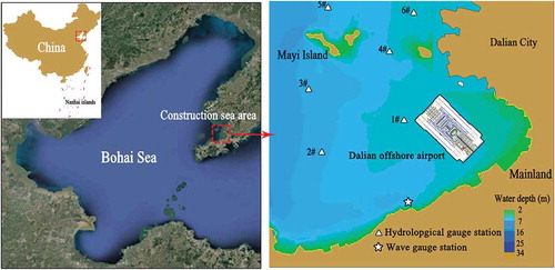
Geographically, the project is located in China’s Bohai Sea, which is a shallow, semi-enclosed sea in the northeastern part of China (37°07′–41°00′N, 117°35′–121°10′E). The Bohai Sea, which has an area of 75,618 km² and an average depth of 18 m, is connected to the adjacent Yellow Sea through the 100-km-wide Bohai Straight. In recent years, the frequent economic activities in the coastal area around the Bohai Sea, combined with the poor water exchange ability of Bohai Sea, have led to the serious deterioration of water quality. To protect the marine environment, it is necessary to closely monitor and prevent the possible pollution during the offshore construction for the protection of the Bohai Sea environment.

Characteristics of tides and currents

The field observations of hydrodynamic characteristics in the CSA were conducted by Wang et al. (2013). The locations of the observation stations are presented in Figure 1. The direction of tidal current around the construction is northeast (NE) during flood tides, whereas the opposite is true during ebb tides. The average and maximum velocity are 0.12–0.25 m/s and 0.21–0.53 m/s, respectively. The average velocity for spring tides and neap tides is 0.21 m/s and 0.14 m/s, respectively.

Characteristics of waves

According to the field measurements, the directions of the prevailing waves around the construction are north (N) and northwest (NW), with a frequency of 15% in N direction and 14% in the NW direction. In addition, the directions of strong waves are also N and NW, with an occurrence frequency of 16% in NW direction and 15% in N direction. Furthermore, in N direction, the mean wave height and the maximum wave height are 0.9 m and 2.7 m, respectively, with a period of 4.2 s. In NW direction, the mean height and the maximum height are 0.6 m and 1.9 m, respectively. The mean heights in other directions are all below 0.7 m, with a period of 1.4–2.6 s.

Methods

Data and processing

In situ sampling

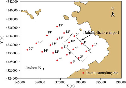
Based on the hydrodynamic characteristics, 20 sampling sites were established approximately 1 km from each other with a grid style in the CSA. The layout of sampling sites is presented in Figure 2. Water samples were obtained by vessel and stored in a freezer. Other parameters including the time of sampling, weather and wind speed were also recorded synchronously. According to the specification of China’s water quality parameters measurement (GB 11901-89), the SPM concentrations were obtained from the water samples by dried-filter weighting method (Filter GN-CA with a 0.45 μm effective pore size). Considering weather conditions and satellite transit time, in situ sampling was conducted 12 times in the CSA from 2012 to 2015, and 240 water samples were obtained.

Figure 2. The location of sampling sites around the offshore construction.

Satellite image data and processing

HJ-1A/1B satellite data were employed to monitor the SPM concentrations in the sea area around offshore construction. HJ-1A/B satellites were launched by China in 2008 to monitor environment and natural disasters. Each of these optical satellites is equipped with two multi-spectrum CCDs. The CCD cameras capture four spectral bands (430–520 nm, 520–600 nm, 630–690 nm and 760–900 nm) with a scan swath of 360 km (≥700 km with two sensors). The constellation of the two satellites generates multi-spectrum CCD images with both a high spatial resolution (30 m) and a short revisit time (2 days) (Tian et al., 2014). In this study, 12 cloudless HJ-CCD images covering the CSA were obtained to monitor the SPM concentrations. The acquisition date of each satellite images is same as that of in situ sampling. The satellite images were obtained from the China Centre for Resources Satellite Data and Applications (CRESDA) (http://www.cresda.com/) and the Satellite Environment Centre of the Ministry of Environmental Protection (SECMEP) (http://www.secmep.cn/).

Radiation calibration, atmospheric correction and geometric correction of HJ-CCD images were performed as follows. (1) The radiometric calibration for HJ-CCD images consists of two steps: first, we converted the DNs (grey scale) to radiance values, and then we converted these radiance values to Top of Atmosphere (ToA) reflectance. The required parameters in the conversion come from the XML format file in HJ-CCD raw data. (2) The atmospheric correction of HJ-CCD image data was performed using the FLAASH module in ENVI 5.2. (3) The initial geometric correction of the HJ-CCD images data was performed referring to 1:100,000 topographic map, and the precise geometric correction was then performed using the measured GPS control point, so that the correction accuracy is less than 1 pixels.

Match-up analysis

Given the extremely short transit time of satellite, few water samples can be collected exactly when the satellite views their location. Therefore, it is necessary to set a time window, and it is assumed that the acquisition of satellite image is synchronized with in situ sampling within the time window. The size of time window has a significant effect on retrieval results: too large time window will increase the uncertainty of retrieval results, while too small will lead to many water samples be ignored. Bailey and Werdell (2006) proposed that the time window can be set to ±3 h around the satellite overpass for open ocean waters. Compared with open ocean waters, the distribution of SPM concentration induced by offshore construction would change faster under the action of tides, wave and wind in coastal waters. Therefore, the time window for the CSA should be less than that for open ocean waters. Based on the analysis above, the time window was set to ±1.5 h around the satellite overpass for the CSA, and was used to select water samples.

Neural network training

For a reclamation project, the SPM induced by the construction has the characteristics of uneven concentration distributions, different particle sizes and rapid shape changes. These characteristics will affect the remote sensing reflectance of the waters, so that the optical properties of the CSA are more complex than that of the waters in the natural state (Cai, Tang, Levy, & Liu, 2016; Cai, Tang, & Li, 2015; Islam, Wang, Smith, Reddy, & Lewis, 2007). In recent years, the artificial neural network (ANN) has been successfully applied to monitor the SPM concentrations in coastal areas under natural conditions (Chebud, Naja, Rivero, & Melesse, 2012; Kazemzadeh, Ayyoubzadeh, & Moridnezhad, 2013; Merrad, Loumi, & Sansal, 2008; Moridnejad et al., 2013). However, it is unknown whether this method can be applied for the construction sea areas. Based on the existing research, this study tries to use ANN model to monitor the SPM concentrations in construction sea areas.

Evaluation of ANN training and test effect

In this study, the root mean square error (RMSE) and mean relative error (MRE) were used to assess the effect of neural network training and testing. The statistics were calculated as follows:

(1)

(2)

where y_i is the calculated value, x_i is the observed value, and N is the number of samples.

Construction of ANN model

The structure of ANN is mainly determined by the mapping relationship between input and output parameters. Therefore, selecting the appropriate input and output parameters is an important part to determine the structure of ANN model. Because the waters in the CSA is slightly and moderately turbid (average SPM concentration is below 35 mg/l), the weak scattering and strong absorption of near infrared (NIR) band by the waters greatly reduce the magnitude of the recorded signal in the NIR region of HJ-CCD satellite, thus reducing the signal–noise ratio (SNR) and enhancing the effect of the inherent noise in the recorded signal (Chen, Quan, Cui, & Song, 2015; Shen, Zhou, Li, He, & Verhoef, 2013). It was also found that there was a low correlation relationship between the measured SPM concentrations and the remote sensing reflectance of NIR band from HJ-CCD satellite. Thus, the NIR band is not suitable for establishing the ANN model for the CSA. Based on the above analysis, the input of the model was set as the remote sensing reflectance of the first three bands of HJ-CCD data, and the output was set as measured SPM concentrations. The activation function for hidden layers was a nonlinear hyperbolic tangent function, while the output node was only equipped with a linear function. The basic architecture of the ANN model used in this study is shown in Figure 3.

Figure 3. Basic architecture of the ANN model used in this study, where Rrs represented remote sensing reflectance.

Training and test dataset for ANN model

After screening with the set time window, there are 210 water samples that can be used to train and test neural network model. The measured SPM concentrations from the water samples ranged from 0.8 to 76.2 mg/l, with an average of 19.3 mg/l. The measured concentrations data were divided into training and test dataset. The training dataset included 132 samples selected from 27 March, 10 September, 27 November 2012, 19 April, 11 August, 28 October 2013, 24 April and 26 November 2014; The test dataset included 78 samples selected from 5 July 2013, 24 June, 11 September 2014 and 22 April 2015. The SPM concentrations in the training dataset ranged from 2.4 to 65.7 mg/l, with an average of 18.22 mg/l; the concentrations in the test dataset ranged from 0.8 to 76.2 mg/l, with an average of 20.91 mg/l (Table 1 and Figure 4). Additionally, the SPM with higher concentrations were usually found around the offshore construction, while the low values were measured in the sea area far away from the construction; the SPM concentrations in winter were higher than that in other seasons.

Table 1. The measured SPM concentrations from water samples in the construction sea area.

Measured SPM concentrations (mg/l)	Min	Max	Median	Average	Standard deviation
Training dataset, 132 samples	2.4	65.7	11.45	18.22	11.45
Testing dataset, 78 samples	0.8	76.2	7.45	20.94	7.5

Figure 4. The number of samples within different concentrations range.

Table 1 The measured SPM concentrations from water samples in the CSA

ANN model training

Due to the optical complex of the waters in the CSA, three types of model architecture were trained: one, two or three hidden layers with the number of neuron nodes varying from 1 to 30. The network was trained using the training dataset and Levenberg Marquardt algorithm. The optimal network architecture was determined with a minimal MRE value and a minimal number of neuron nodes. Based on 132 field samples in the training dataset, the model in Figure 3 was determined as the optimal ANN model to retrieval SPM concentrations from the waters in the CSA. For the SPM in the training dataset (2.4–65.7 mg/1), the ANN model showed good statistical results as shown in Figure 5. The linear slope and determination coefficient between the calculated and measured value were 0.98 and 0.97, respectively. Based on the determination coefficient, the ANN model can account for 97% variation of SPM concentrations in the CSA.

Figure 5. Optimal ANN model initialized from the training dataset (n = 132) .

Numerical model for SPM distribution

To predict the distribution of SPM concentrations during the construction, a 2D tidal current numerical model and a water quality model should be established based on the hydrodynamic characteristics of the CSA. The boundary conditions of the tides and currents for the CSA were provided by the hydrodynamic mathematical models of the Yellow Sea and Bohai Sea derived from the ECOMSED model. The wave parameters for the CSA were computed by the wave model and were used to provide the wave’s radiation stress coefficient for the 2D tidal current numerical model (Baumert et al., 2000). Field observed data of tide height, flow velocity and flow direction were used to calibrate and validate the models. Consequently, a water quality model was developed to calculate the diffusion of the SPM induced by the offshore construction based on the validated tidal current numerical model.

Tidal current mathematical model

As mentioned earlier, the CSA is a wide and shallow bay. The horizontal scale of the CSA is much larger than the vertical scale, and the change of the hydraulic parameters along the vertical direction is much smaller than that along the horizontal direction (Wang et al., 2013; Yan et al., 2014). Therefore, the two-dimensional tidal current mathematical model based on a mean water depth is suitable for hydrodynamic calculations in the CSA. The model developed by Sankaranarayanan and Mccay (2003) is as follows:

(3)

(4)

(5)

(6)

where u and v are the current velocities in the x and y directions, respectively (m/s); z is the water level (m); z₀ is the elevation of seabed (m); h is the total water depth (m) and is the sum of z and z₀; w_x and w_y represent the wind velocity in the x and y directions, respectively (m/s); f is the Coriolis coefficient (s⁻¹); C_w is the shear coefficient of the wind to wave and is 2.5510⁻³ (N/m⁻³); A_x and A_y are eddy viscosity; τ_b is the bottom shear stress under the co-action of waves and currents (N/m⁻²). The components in the x and y directions are calculated as follows:

(8)

where u_w and v_w are the bottom particle velocities of waves, with u_w = 0, v_w = 0 for the case without wave effects (m/s); C_s is the Chezy coefficient, where C_s =  (1/n)h^1/6; n is the roughness coefficient; B is the interaction coefficient between waves and currents (0.359); and f_w is the bottom friction coefficient of the wave.

Water quality model

Based on the validated tidal current model, a 2D water quality model was added to predict the distribution of SPM concentrations induced by the offshore construction. During construction, coarse particulate matter settles rapidly, while fine particulate matter (grain size less than 0.03 mm) is suspended in seawater and is gradually diffused under the action of the tides and currents. Thus, the process of settlement is neglected in this study. The water quality equation is shown as follows (Zhu & Ying, 2009; Yan, Wang, Yu, & Song, 2015):

(9)

where D_x and D_y are pollution diffusion coefficients in the x and y directions, respectively (m²/s); c is the pollutant concentration (kg/m³); F is the attenuation coefficient and is equal to zero; s is the pollutant source intensity (kg/s).

Results and analysis

Accuracy evaluation of ANN model

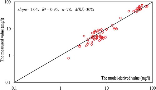
To evaluate the accuracy of the ANN model, the calculated SPM concentrations derived from the model were compared with the measured values in the test dataset, as shown in Figure 6. For the SPM in the testing dataset (0.8–76.2 mg/1), the mean relative error (MRE) of the calculated value obtained by the ANN model was not more than 98%, with an average of 30%. The linear slope and the determination coefficient between the calculated and measured value are 1.05 and 0.95, respectively. Therefore, the established ANN model can accurately retrieve the SPM concentrations from the waters in the CSA, where the optical properties are quite complex due to the offshore construction.

Figure 6. Comparison of the calculated SPM concentrations derived from the model with the measured value in the testing dataset (n = 78).

Distribution of the SPM from numerical model

Model solution and verification

The tidal model covered the CSA with an unstructured triangular mesh. The model boundaries included the water–land boundary (closed boundary) and the water–water boundary (open boundary). For the closed boundary, the flow flux in the outward normal direction was zero. The open boundary was given by the known hydrodynamic parameters. To validate the model, the model results were compared with the field observed data of the tide height, flow velocity and direction from the hydrological station (1#) in the CSA. A comparison of the model results with field observed data showed a reasonable correlation (not shown) (Wang et al., 2013).

For the water quality model, the initial condition was C(x,y)|_t=0 = 0 because this study focused on the SPM induced by the offshore construction and ignored the background concentration. The concentration flux in the closed boundary was zero, and the inflow condition at the open boundary was C|_Γ = P₀, where Γ was the water boundary and P₀ was the boundary concentration. In this study, P₀ was equal to zero. The outflow condition at the open boundary was ∂C/∂t+ U_n∂C/∂n^w = 0, where n is the normal direction of boundary and U_n is flow velocity in direction n.

The modelled SPM distribution induced by the construction

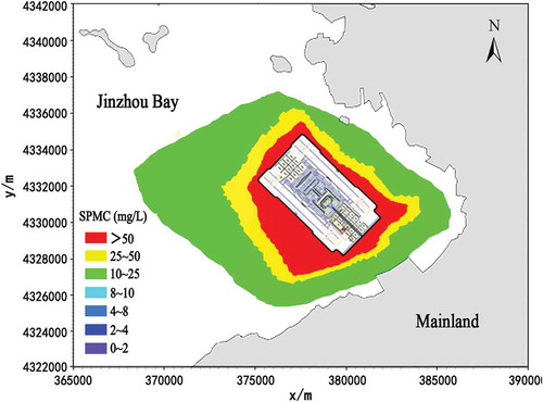
Using the water quality model, the simulated accumulative envelope diagram of the maximum dispersion range of the SPM induced by the construction was obtained, as shown in Figure 7. The diffusion range of the SPM induced by the construction is approximately 105.15 km², among which the area with concentrations of 10–25 mg/l accounts for 63% and is 66.8 km². The area with concentrations of 25–50 mg/l accounts for 17% and is 17.36 km², and 20% had concentrations above 50 mg/l.

Figure 7. Simulated accumulative envelope diagram of maximum dispersion range of SPM induced by the construction.

Comparison between the results from remote sensing and numerical model

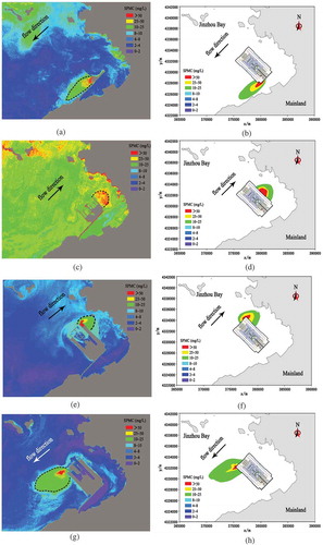
The distribution of SPM concentrations in the CSA was derived from the ANN model, as shown in Figure 8a, c, e and g. From the satellite images, it can be seen that the SPM concentrations in the sea areas near the reclamation construction are high (greater than 10 mg/l), while the concentrations in other sea areas are relatively low (below 10 mg/l); the SPM concentrations in winter were slightly higher than that in other seasons. The distributions of SPM concentrations derived from satellite images were consistent with the results from the measured value. Additionally, the diffusion direction of the SPM plumes induced by the construction was consistent with the direction of tidal current in the sea areas. The numerical model was also used to simulate the SPM concentrations induced by the construction at the acquisition time of HJ-CCD image, as shown in Figure 8b, d, f and h. The modelled SPM distribution showed a qualitatively similar pattern with the results obtained by remote sensing. It should be noted that, the concentrations of SPM induced by the construction on 5 December 2013 were underestimated in the numerical model (Figure 6b) compared to satellite image, which can be explained by the large wind speed in winter (>10 m/s). The analysis of remote sensing images and numerical model results indicated that the concentrations and distribution patterns of SPM induced by the offshore construction mainly depended on the reclamation activity, tidal currents and wind speed. It should be noted that, the SPM concentrations obtained by remote sensing in this study are the results from the co-action of various factors (construction, wind, tide and rainfall), while that obtained by the water quality model is only induced by the reclamation construction. Thus, the results obtained by two methods cannot be compared quantitatively at present (Sipelgas, Raudsepp, & Kõuts, 2006). How to extract the SPM concentrations induced by reclamation construction using remote sensing technology, and how to compare the results quantitatively will still require us to further study.

Figure 8. Distribution of SPM concentration (mg/l) from ANN model and numerical model.

In conclusion, the technical method used in this study provides important information to assist in reducing environmental pollution during the reclamation construction. During the construction of the Dalian offshore artificial island, Dalian government has monitored the diffusion and distribution of SPM with the combining method. Based on the monitoring results, the government formulated a series of environmental protection measures: the construction should be avoided during ebb tides to reduce the diffusion of SPM; the construction should also be avoided during the growth and spawning seasons for benthic organisms, fish and zooplankton; concurrently, the reclaimed materials should be stone-based, and contain no more than 10% of miscellaneous soils. These measurements have been proved to be effective in reducing the marine environmental pollution during the construction.

Conclusion

Taking the construction of the Dalian offshore artificial island as a background, the distribution of SPM induced by the construction was predicted using numerical model. Concurrently, an ANN model was established with satellite data and in situ measurements to calibrate the numerical simulation results. This case study shows that, using numerical modelling and remote sensing can provide effective information for the monitoring of marine environment during offshore construction. Furthermore, the following conclusions were drawn.

(1) According to the hydrodynamic characteristics of the CSA, a two-dimensional hydrodynamic model and a water quality model were used to simulate the distribution of SPM induced by the offshore construction. The dispersion range of SPM induced by the construction was approximately 105.15 km², among which 63% of the area had concentrations between 10 and 25 mg/l, 17% had concentrations between 25 and 50 mg/l, and 20% of the area had concentrations above 50 mg/l.

(2) Due to the complex optical properties of the CSA, an ANN model for retrieving SPM concentrations was established based on the reflectance data from HJ-1A/1B-CCD satellite image and the measured SPM concentrations in the CSA. The relative error (RE) of the calculated value obtained by the model was not more than 98%, with an average of 30%. Therefore, the established ANN model can accurately retrieve the SPM concentrations from the waters in the CSA.

(3) Good agreement was found between the results from numerical modelling and the retrieval. Thus, the simulated SPM distribution induced by the construction was considered credible. When the distribution of SPM concentrations cannot be derived from the satellite data due to weather conditions, the numerical model can be used to simulate the SPM distribution in the sea area around the construction.

Through the above work, the effective monitoring of the SPM concentrations induced by the construction of the offshore airport artificial island over large areas is successfully achieved, which provides a scientific basis for the development of environmental protection scheme during the construction period. The case study provides a method for monitoring of environmental pollution induced by offshore construction, and serves as a reference for other similar offshore engineering.

Acknowledgments

Sincere thanks to the reviewers for their very useful comments on this paper.

This research was supported by the National Ocean Soft Science Project (Grant No. JJYX201612-1). The authors thank all the people involved in this project and the volunteers who provided information to us.

Disclosure statement

No potential conflict of interest was reported by the authors.

Additional information

Funding

This work was supported by the National Ocean Soft Science Project [JJYX201612–1];

References

- Bailey, S.W., & Werdell, P.J. (2006). A multi-sensor approach for the on-orbit validation of ocean color satellite data products. Remote sensing of environment, 102(1–2), 12–23.
- Baumert, H., Chapalain, G., Smaoui, H., Mcmanus, J.P., Yagi, H., Regener, M., ... Szilagy, B. (2000). Modelling and numerical simulation of turbulence, waves and suspended sediments for pre-operational use in coastal seas. Coast Engineering, 41(1–3), 63–93.
- Cai, L.N., Tang, D.L., Levy, G., & Liu, D.Y. (2016). Remote sensing of the impacts of construction in coastal waters on suspended particulate matter concentration - the case of the Yangtze River delta, China. International journal of remote sensing, 37(9), 2132–2147.
- Cai, L.N., Tang, D.L., & Li, C.Y. (2015). An investigation of spatial variation of suspended sediment concentration induced by a bay bridge based on Landsat TM and OLI data. Advances in space research : the official journal of the Committee on Space Research (COSPAR), 56(2), 293–303.
- Carmo, J.S.A.D., & Seabra-Santos, F.J. (2002). Near-shore sediment dynamics computation under the combined effects of waves and currents. Advances in engineering software (Barking, London, England : 1992), 33(1), 37–48.
- Chebud, Y., Naja, G.M., Rivero, R.G., & Melesse, A.M. (2012). Water Quality Monitoring Using Remote Sensing and an Artificial Neural Network. Water Air Soil Poll, 223(8), 4875–4887.
- Chen, J., Quan, W.T., Cui, T.W., & Song, Q.J. (2015). Estimation of total suspended matter concentration from MODIS data using a neural network model in the China eastern coastal zone. Estuar Coast Shelf S, 155, 104–113.
- Dogliotti, A., Ruddick, K.G., Nechad, B., Doxaran, D., & Knaeps, E. (2015). A single algorithm to retrieve turbidity from remotely-sensed data in all coastal and estuarine waters. Remote sensing of environment, 156, 157–168.
- He, M.X., Hu, L.B., & Hu, C.M. (2014). Harbour dredging and fish mortality in an aquaculture zone: Assessment of changes in suspended particulate matter using multi-sensor remote-sensing data. International journal of remote sensing, 35(11–12), 4383–4398.
- Hellweger, F.L., Schlosser, P., Lall, U., & Weissel, J.K. (2004). Use of satellite imagery for water quality studies in New York Harbor. Estuar Coast Shelf S, 61(3), 437–448.
- Hemer, M.A., Harris, P.T., Coleman, R., & Hunter, J. (2004). Sediment mobility due to currents and waves in the Torres Strait–Gulf of Papua region. Continental shelf research, 24(19), 2297–2316.
- Islam, A., Wang, L., Smith, C., Reddy, S., & Lewis, A. (2007). Evaluation of satellite remote sensing for operational monitoring of sediment plumes produced by dredging at Hay Point. Journal of applied remote sensing, 1, 11506.
- Kazemzadeh, M.B., Ayyoubzadeh, S.A., & Moridnezhad, A. (2013). Remote sensing of temporal and spatial variations of suspended sediment concentration in bahmanshir estuary, iran. Indian Journal of Science & Technology, 6, 5036–5045.
- May, C., Koseff, J., Lucas, L., Cloern, J., & Schoellhamer, D. (2003). Effects of spatial and temporal variability of turbidity on phytoplankton blooms. Marine Ecology Progress, 1(254), 111–128.
- Merrad, H., Loumi, S., & Sansal, B. (2008). Modeling of Suspended Particulate Matter in the Algerian Coast Using Neural Networks and Mathematical Morphology. International Journal of Computer Science & Applications, 5, 33–40.
- Min, J., Ryu, J., Lee, S., & Son, S. (2012). Monitoring of suspended sediment variation using Landsat and MODIS in the Saemangeum coastal area of Korea. Marine pollution bulletin, 64(2), 382–390.
- Moridnejad, A., Abdollahi, H., Alavipanah, S.K., Samani, J.M.V., Moridnejad, O., & Karimi, N. (2013). Applying artificial neural networks to estimate suspended sediment concentrations along the southern coast of the Caspian Sea using MODIS images. Arabian Journal of Geosciences, 8, 891–901.
- Onderka, M., & Pekarova, P. (2008). Retrieval of suspended particulate matter concentrations in the Danube River from Landsat ETM data. The Science of the total environment, 397(1–3), 238–243.
- Pugliese, C.E.E., Dentale, F.F., & Reale, F.F. (2011). On the Effects of Wave-Induced Drift and Dispersion in the Deepwater Horizon Oil Spill. Geophysical Monograph, 195, 197–204.
- Sankaranarayanan, S., & Mccay, D.F. (2003). Application of a two-dimensional depth-averaged hydrodynamic tidal model. Ocean Engineering, 30(14), 1807–1832.
- Shen, F., Zhou, Y.X., Li, J.F., He, Q., & Verhoef, W. (2013). Remotely sensed variability of the suspended sediment concentration and its response to decreased river discharge in the Yangtze estuary and adjacent coast. Continental Shelf Research, 69, 52–61.
- Sipelgas, L., Raudsepp, U., & Kõuts, T. (2006). Operational monitoring of suspended matter distribution using MODIS images and numerical modelling. Advances in space research : the official journal of the Committee on Space Research (COSPAR), 38(10), 2182–2188.
- Song, K.S., Li, L., Wang, Z.M., Liu, D.W., Zhang, B., Xu, J.P., et al. (2012). Retrieval of total suspended matter (TSM) and chlorophyll-a (Chl-a) concentration from remote-sensing data for drinking water resources. Environmental Monitoring and Assessment, 184(3), 1449–1470.
- Tian, L., Wai, O., Chen, X., Liu, Y., Feng, L., Li, J., et al. (2014). Assessment of Total Suspended Sediment Distribution under Varying Tidal Conditions in Deep Bay: Initial Results from HJ-1A/1B Satellite CCD Images. Remote Sens-Basel, 6(10), 9911–9929.
- Wang, N., Yan, H.K., Liu, Z.B., Tong, S.Q., Yu, T.L., & Liang, C. (2013). Effects of Different Layout Schemes on the Marine Environment of the Dalian Offshore Reclaimed Airport Island. Journal Environment Engineering, 139(3), 438–449.
- Wu, G.F., Liu, L.J., Chen, F.Y., & Fei, T. (2014). Developing MODIS-based retrieval models of suspended particulate matter concentration in Dongting Lake, China. International Journal Applications Earth Obs, 32, 46–53.
- Yan, H.K., Wang, N., Yu, T.L., & Fu, Q. (2014). Simulation of different sea-crossing traffic route structures’ effects on the marine environment for the Dalian large-scale offshore airport island. Journal Hydraul Researcher, 52(5), 583–599.
- Yan, H.K., Wang, N., Yu, T.L., & Song, N.Q. (2015). Hydrodynamic Behavior and the Effects of Water Pollution from Dalian’s Large-Scale Offshore Airport Island in Jinzhou Bay, China. Journal Waterway Port Coast, 141(1), 05014003.
- Zhu, J., & Ying, C. (2009). Application of 2D dynamic water quality model to the upstream Qiantang estuary. Journal of Hydroelectric Engineering, 28(6), 157–161.