Contribution of the UAS to the determination of the water budget in a coastal wetland: a case study in the natural park of the Bay of Cádiz (SW Spain)

ABSTRACT

Wetlands are sensitive and complex systems whose conservation is a priority. For the correct understanding of their hydrological dynamics, it is necessary to determine the different elements of the water budget and, in particular, the geometry of the wetland basin in order to estimate the variations in storage capacity. This paper presents a novel, low-cost, user-friendly photogrammetric technique to obtain high-resolution datasets using non-metric cameras located in unmanned aerial systems (UAS) and structure-from-motion algorithms for producing high-precision 3D point clouds. The accuracy of the cartographic products obtained is evaluated using 59 checkpoints and comparing with the available LiDAR models. Best results are obtained using a full frame RGB sensor, which results in an orthomosaic with a pixel size of 1.38 cm and a positional RMSE of 3.8 cm in horizontal and a digital surface model (DSM) with a 3.5 cm RMSE_Z. From the DSM, eliminating the influence of vegetation through masks, a digital terrain model (DTM) with a 5.9-cm RMSE_Z that allows defining the filling curve of the wetland basin is obtained. This curve relates the stored volume and the surface exposed to evaporation with the water level, which allows to perform simulations in the balance models.

KEYWORDS:

• Wetlands
• water budget
• unmanned aerial systems (UAS)
• low-cost photogrammetry
• structure from motion
• digital terrain model (DTM)

Introduction

Wetlands are among the most important but most threatened environmental resources in the world. The interest of wetland conservation is centered in several aspects: on one hand, the maintenance of the functioning of the ecosystems and the natural processes operating in these areas: hydrological transfers and storage of water, biogeochemical transformations, primary productivity, decomposition, and community/habitat conservation (Richardson, 1994); and on the other hand, the benefits generated to the society and the natural environment. Therefore, the need for rational use and conservation stems from the recognition of the high-value goods and services that these ecosystems provide to the society (Maltby, 1991).

A basic aspect for the conservation and management of wetlands is the understanding of their hydrology and, in particular, the definition of their water budget, which expresses the movement of water that feeds, leaves and is stored in the wetland (Mekiso, Ochieng, & Snyman, 2016; Owen, 1995). Various methodologies have been proposed for monitoring the different elements of the balance (Gilvear & Bradley, 2000), but the quality of the model depends, to a great extent, on the correct definition of the morphology of the water storage basin (Moral, Rodríguez-Rodríguez, Benavente, & Cifuentes, 2009). From this and with a control of the water level, it can be determined the flooded surface and the variation in water storage over time, as it has been described by García-López, Ruiz-Ortiz, and Muñoz-Pérez (2018) for other hydrosystems. Thus, the estimation of certain elements of the balance such as the direct evaporation, the contribution of the surface runoff or the water transferred to the aquifer, can be performed directly. In the case of coastal wetlands, it is also critical to accurately define their elevation relative to the sea level in order to assess the influence of tides and high-energy coastal phenomena on wetland dynamics.

The morphology of the basin of a wetland can be defined by traditional procedures: bathymetry in high water situations or direct surveying with leveling instruments, aerial or satellite photogrammetry in low water situations. In all cases, it is difficult to obtain a definition of the geometry of the basin with enough resolution. Although centimeter-scale accuracies can be obtained in height (Z-coordinate) by means of direct measurements with adequate instrumentation (differential GNSS, total station), this type of field operations became very laborious, even more in the case of obtaining high density information. On the other hand, using aerial photogrammetry or airborne LiDAR, the Z-coordinate accuracies are usually not lower than 10 cm.

However, with the advent and popularization of unmanned aerial systems (UAS), progress has been made in leading to the development of rapid and low-cost very high-resolution studies, although coverage is significantly lower respect to traditional remote sensing systems (satellite or aerial).

Precision aerial photogrammetric techniques with low-cost sensors have recently been applied in numerous detailed hydrological studies, with results that improve those obtained with traditional techniques (Madden et al., 2015). Numerous researchers find that these techniques provide more accurate–precise, low-cost and less time-consuming geomatic products: DeBell, Anderson, Brazier, King, and Jones (2016) made a review of the application of UAS to water resources management (WRM), focused on a range of pragmatic concepts and on aspects such as, the types of UAS, sensor payloads, data processing and application examples in water management. Leitão, Moy de Vitry, Scheidegger, and Rieckermann (2016) exposed the applicability and the advantages of using UAS to generate very high resolution digital elevation models (DEM) to be used in urban overland flow and flood modeling. Nobajas, Waller, Robinson, and Sanzongalo (2017) described the characterization of a small badland drainage basin using an unmanned rotorcraft to obtain a high definition orthophotography and DEM, processed using structure from motion (SfM) photogrammetric software. In fluvial geomorphology, Zazo, Molina, and Rodríguez-Gonzálvez (2015) proposed the application of an innovative technique called RC-APP (Reduced Cost Aerial Precision Photogrammetry) that uses as aerial platform an ultra-light aircraft to get a better geometric definition of the flood area. Tamminga, Eaton, and Hugenholtz (2015) analyzed three-dimensional morphodynamic changes and patterns of erosion and deposition associated with an extreme flood event using orthophotograpy and DEMs produced from multi-temporal datasets collected with UAS. Lejot et al. (2007) focused the application of these techniques to the definition of channel water depth and gravel bar geometry and Vázquez-Tarrío, Borgniet, Liébault, and Recking (2017) characterized grain roughness and size distribution in a braided, gravel-bed river. Woodget, Austrums, Maddock, and Habit (2017) showed the contribution of UAS and digital photogrammetry for monitoring physical river habitat and hydromorphology. Regarding wetlands studies, Chabot and Bird (2013) and Chabot, Carignan, and Bird (2014) used a small UAS to acquire aerial imagery and characterize land cover in a wetland and impoundment as part of a conservation study of the least bittern (Ixobrychus exilis); they identify the fine-scale water–vegetation interface in which several types of vegetation could be distinguished and classified using spectral image analysis software. Finally, Boon et al., (2016) showed results of a study using UAS as a photogrammetry tool for mapping wetlands and to obtain terrain features and derive ultra-high-resolution point clouds, orthophotos and 3D models, from multiple photos with centimeter accuracy.

This work presents the results of an aerial photogrammetric survey using UAS with the aim of defining the geometry of the wetland basin and establishing the relationship between the stored volume, the surface of water sheet and the water level. For this purpose, a hydrological situation of low water is necessary. Two surveys were performed with two UAS with different performances. In each of them, the accuracy and precision are evaluated and the results compared with the official cartographic documents available for the area, produced from photogrammetric flights and airborne LiDAR sensors.

Case study

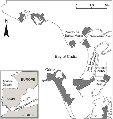
The study area is located on the Atlantic coast of Andalusia (SW Spain), in the system of islands-barrier that forms the Bay of Cádiz. Specifically, it is located in the sector of Los Toruños and Pinar de la Algaida, on the left bank of the San Pedro River tidal channel (Figure 1). The topography of the region is very smooth and the hydrodynamic regime is mesomareal, with maximum tidal ranges of 3.7 m, which conditions the typology and characteristics of the sedimentary deposits. In the study area, fine-grained recent detrital materials, typical of beach environments with aeolian and fluvial influences, are recognized. Muddy materials typical of marshland also outcrop. Sedimentation during the Holocene is largely controlled by sea level fluctuations, tectonic structure, and late tectonic readjustments of the Betic Cordillera (Gutiérrez-Mas & García-López, 2015).

Figure 1. Location of the studied area.

The climate context is Mediterranean with Atlantic influences. The average annual precipitation is close to 600 mm, with a markedly seasonal distribution, mainly concentrated in late autumn and winter, and dry summers. The average annual temperature is 18.2°C with mild winters (monthly average of 12.8°C in January) and hot summers (average monthly of 24.5°C in August).

From the conservation point of view, the study area belongs to the Bahía de Cádiz Natural Park, a protected area with a surface of about 10,500 ha. It has been included since 2002 in the List of the RAMSAR Convention on Wetlands of International Importance. In addition, this protected area has been considered since 2003 as a Special Protection Area for Birds (SPAB) because of its relevance for the maintenance of habitats and species of interest (Junta, 2017).

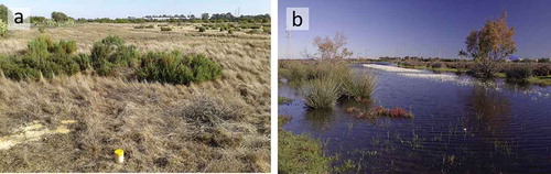
Although the study area is located in a very artificialized environment, surrounded by road infrastructures, urbanized areas, services and industrial areas, and despite its small size (<200 ha), it has a high environmental uniqueness due to the diversity of existing environmental units: marsh, fixed dune with coastal pinewood, meadows, and temporary or permanent flooding with fresh or brackish water with different salinity (Figure 2). This last characteristic confers to the area a great variety of aquatic habitats, changing in time, which favors the conservation of the ecological communities. Five temporary ponds, showing very different characteristics in terms of hydrochemical water quality and hydroperiod, have been identified (García de Lomas, García, & Canca, 2004). These authors perform a detailed inventory of species, some of which are endemic, rare or threatened. In this small area, they identify 118 plant species and a large number of invertebrate species that support a wide seasonal bird community. The concentration of this genetic diversity of species, some of them very specialized and characteristic of physically forced systems, give a special interest to the study area from a conservation, scientific and educational point of view (Pérez Hurtado & García-Jiménez, 2004).

Figure 2. Views of the studied area. (a) Aspect of the study area during the dry season; in the foreground a piezometer of the hydrological control network can be observed. (b) The study area flooded after the rain season.

Among the threats identified in the above mentioned temporary ponds are the following: (1) the decrease in the groundwater levels of the aquifer caused by pumping to prevent leakage in basements of some buildings in the area; (2) the reduction of surface inputs by channels constructed in areas of recent urbanization, (3) the reduction of the surface recharge of the aquifer related to (2) and (4) the spread of pollutants from a former urban solid waste transfer facility, which was operative until the late 1990s in areas adjacent to the Natural Park. In addition, the incidence of climatic variability must be taken into account, as the last three hydrological years have been drier than the average and the surface storage in the wetland has been especially scarce and ephemeral. This has caused the colonization of shrub vegetation from previously flooded areas and a smaller influx of avifauna. Consequently, there has been concerns in Park managers who question whether the natural dynamics are being affected by the indicated pressures.

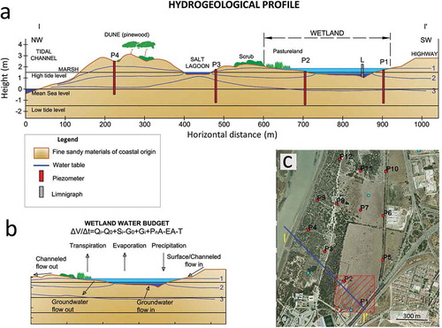
In order to understand the relationship between the wetland and the underlying sandy aquifer, a piezometric control network was deployed in 2015 (García-López et al., 2016), which has provided valuable information on the hydrodynamics of the groundwater (Figure 3). In addition, a systematic control is being carried out on the level of the water sheet in the Laguna de la Vega in order to adjust the water balance. A clear dependence on the durability of the lagoon with respect to the state of storage of the aquifer has been identified. When the piezometric levels are high, infiltration losses are reduced and the main water outlet of the wetland is by evaporation. However, when piezometric levels are low, evaporation becomes less important and the lagoon is emptied by infiltration through the permeable bed, until hydraulic equilibrium with the aquifer is acquired. However, it is essential to have accurate information on the morphology of the basin for evaluating the volume differences involved in the different elements of the balance and also to know the flooded surface at any given time. In this paper, the results of a high-resolution photogrammetric survey using UAS in the Laguna de la Vega, the most significant pond in the area, are presented.

Figure 3. (a) Hydrogeological profile with indication of the water table in three hydrological situations: (1) situation in a rainy year, (2) normal year and (3) prolonged dry season. (b) Wetland water budget scheme. (c) Location of the hydrological control network on aerial photography taken during the dry season.

The application of this methodology in this particular case is challenging for several reasons: (1) the basin has an extremely low topography with a 0.8 m range of elevations (between 1.6 and 2.4 m.a.s.l.) and slopes generally less than 0.001; (2) the presence of permanent and seasonal vegetation which makes the definition of the terrain forms difficult, requiring the development of data processing techniques in order to eliminate their effect in the digital surface model (DSM).

Materials and methodology

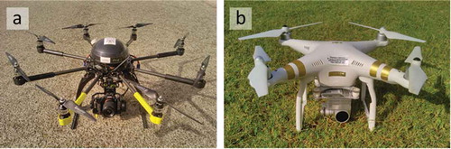
Two photogrammetric flights have been made using UAS equipped with RGB cameras of different characteristics. The first was made with an ATYGES FV-8 high-performance octocopter, with a payload of <5 kg, equipped with a Sony Alpha 7 camera. The second flight was made with a DJI Phantom 3 Professional lightweight quadricopter, with a payload of <0.5 kg, equipped with a camera with a Sony EXMOS sensor (Figure 4). In both cases, a stabilization system (gimbal) for the camera was used. The main characteristics of the cameras are shown in Table 1.

Table 1. Main features of the used cameras.

	Sony Alfa 7	DJI professional
Camera lens	Sony FE	DJI
Focal length (mm)	28–70 (adjusted to 34 mm)	3.1
FOV (°)	75–34	94
Spectral type	RGB	RGB
Sensor type	Full frame CMOS	EXMOS
Sensor size (mm)	35.80 x 23.90	6.16 x 4.62
Resolution (effective pixels)	24.3 MP	12.76 MP
Image size (pixels)	6000 x 4000	4000 x 3000
Pixel size (µm)	5.97	1.57

Figure 4. View of the two equipment used in this work: (a) ATYGES FV-8 octocopter and (b) DJI phantom 3 professional quadricopter.

The work was made in the following five steps.

Flight planning

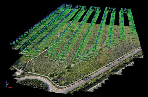
For the FV-8 system, the photographic planning was carried out with the PrePlan software, which helped to select the flight parameters: flight altitude, focal length, velocity, forward and transverse overlap, all based on GSD (Ground Sampling Distance) which was intended to be obtained (<1.5 cm). The generation of waypoints and the flight path for automatic flight was generated with Mikrocopter software. For the Phantom system, the planning was done using the DJI Go software, both for the definition of the flight parameters that in this case were adjusted to obtain a GSD greater than the previous one (<5 cm), as well as to supply the aerial vehicle the necessary data for the automatic execution of the flight. In both cases, the forward and transverse overlap were adjusted to 80% and 60 %, respectively, and the flight altitude was set at 60 m. Also in both cases, the exposure, white balance and ISO were configured in automatic mode, as light conditions did not suffer substantial changes during the execution of the flights. The planned flight pattern for the FV-8 system is shown in Figure 5.

Figure 5. Flight pattern with the location of the photographs over the produced 3D point cloud (FV-8 system). Green circles: predicted shooting points, blue circles: real shooting points.

Data acquisition

After obtaining the corresponding permits, particularly from the Directorate of the Natural Park, two flights were carried out consecutively according to the planning on the 17 April 2017, beginning at 17:30, with a duration of 13 min for the first (FV-8) and 20 min for the second (Phantom). 305 and 157 images were obtained with FV-8 and Phantom systems, respectively, 100% of which were optimal for use in photogrammetric processing.

In order to subsequently geo-reference the photogrammetric model to the coordinate system UTM 29N WGS84 (EPSG 32,629), 11 ground control points (GCP) were evenly distributed on the ground before the flights were performed and their three-dimensional coordinates were measured. For this, a Global Navigation Satellite System (GNSS) observation has been used, with a bi-frequency receiver Leica System 900 GNSS as rover and reference station UCA1 13455M002, of the regional GNSS network (RAP, 2017). Through the real-time differential corrections received from the reference station, mean accuracies of 0.5 cm in X and Y and 0.8 cm in Z in GCP were obtained. The distribution of GCP is shown in Figure 6. The points were previously marked with black and white targets clearly visible in the image.

Figure 6. Position of GCP and checkpoints on the studied area. Red dots are GCP, blue square are checkpoints for geometric validation and yellow dots are checkpoints to evaluate the error of the DTM in the areas occupied by vegetation.

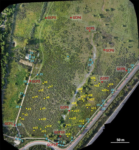
After processing of the data, a second field campaign was carried out to establish the 3D coordinates of 29 checkpoints selected in the produced orthophotography, for the geometric control and accuracy assessment of the 3D model. This was made using the GNSS procedure indicated above with similar precisions. These points, which are different of the GCP, were distributed in the range of altitudes of the terrain, between 1.6 and 2.5 m, on features clearly identifiable in the produced high-resolution orthomosaic (Figure 6).

In addition, after processing of the data, a third field campaign was carried out following the same guidelines as the previous ones with the objective of obtaining the three-dimensional coordinates of 30 new points located on the ground, in positions hidden by the vegetation, with the intention of verifying the interpolation algorithms after the vegetation filtering (Figure 6).

Photogrammetric processing

At this stage, orthomosaic and 3D geometric wetland basin model reconstruction take place through photogrammetry using SfM algorithms. SfM differs from traditional photogrammetry as it does not require reference targets or a priori knowledge of the camera exposure locations and attitudes. Instead, the geometry of the camera and photographs parameters is solved automatically with very little user interaction (Madden et al., 2015). By using multiple overlapping images, SfM incorporates simultaneous, highly redundant, iterative bundle adjustment procedure based on a database of features automatically extracted from a set of multiple overlapping images (Snavely, Seitz, & Szeliski, 2008). The camera positions derived from SfM lack the scale and orientation provided by ground-control coordinates, unlike traditional photogrammetry. Consequently, the 3D point clouds are generated in a relative coordinate system (image-space), which must be aligned to a real world (object-space) coordinate system. The transformation of SfM image-space coordinates to an absolute coordinate system can be achieved using a 3D similarity transform based on a small number of known GCPs with known object-space coordinates (Westoby, Brasington, Glasser, Hambrey, & Reynolds, 2012).

The processing was done using the Pix4D software with the template for 3Dmaps. Pix4D is a photogrammetric software created in 2011 by a Swiss company of the same name. The Pix4D workflow consists of three steps: initial processing, point cloud densification, and DSM and orthomosaic generation. The user-defined properties which guide the quality, accuracy, and format of the final output are all handled through a processing options dialogue box which must be set up prior to any processing steps. Table 2 shows the main characteristics of the processing performed on the images obtained.

Table 2. Results processed with Pix4D Mapper.

	FV-8 system	Phantom system
Area covered (ha)	13.33	14.27
Number of images	305	157
Average GSD (cm)	1.38	3.34
Keypoints per image (median)	88,241	54,640
Matches per calibrated image (median)	43,076.9	27,335.4
Georeferencing Number of GCP Mean RMS error in GCP (m)	11 0.0098 (X) 0.0079 (Y) 0.0107 (Z)	10 0.0295 (X) 0.0327 (Y) 0.0490 (Z)
Number of 2D keypoint observations for bundle block adjustment	12,709,676	4,239,443
Number of 3D points for bundle block adjustment	4,595,853	1,520,142
Mean reprojection error (pixels)	0.133	0.230

Geometric control and accuracy assessment

The results obtained in the previous phase with the ground-truth obtained from the checkpoints (n = 29) were compared. In the orthomosaic with higher spatial resolution (FV-8), the positional accuracy has been evaluated comparing the planimetric coordinates of checkpoints measured in the field with those obtained from the produced orthomosaic. This work has been possible due to the excellent resolution of this product (GSD = 1.38 cm) which has allowed to establish an unequivocal relationship between the checkpoints and their images. As for the DSM obtained with both UAS, the altimetric accuracy was evaluated by comparing with the Z-coordinate of the checkpoints. In addition, a comparison with the most accurate official cartographic product, the LiDAR DTM, was made. In Spain, the National Plan of Aerial Orthophotography (PNOA: Plan Nacional de Ortofotografía Aérea) and the application of directive INSPIRE, Infrastructure for Spatial Information in the European Community (CSG, 2017) allows getting digital aerial orthophotos with resolution of 25 or 50 cm and LiDAR DTM, at ground level (root mean-squared error, RMSE ± 0.50 m), with initial density of 0.5 points/m² and update period of 2–3 years (IGN, 2017).

Postprocessing

After evaluating the geometric quality of the products generated and according to the specific requirements of the hydrological application under study, the DSM with the highest geometric quality (FV-8) was selected to generate a DTM by eliminating the vegetation cover from the model using procedures of digital treatment. This was performed with free software gvSIG 2.2. It should be noted that the DTMs generated automatically by the Pix4D software have not provided acceptable results.

Various authors have proposed methodologies for the automatic identification and classification of vegetation in remote sensing. Most of them are based on the spectral signature of the vegetation and its high reflectance in the near-infrared spectral region (Adam, Mutanga, & Rugege, 2010; Xie, Sha, & Yu, 2008). Methodologies applicable to color images registered in the visible region have also been proposed, although in this case it is a complex task especially when noises and shadows exist in the images (Zheng, Zhang, & Wang, 2009). Methodologies based on the analysis of forms have also been proposed for the identification of vegetation, especially in the case of arboreal vegetation (Wolf & Heipke, 2007).

On the other hand, ground-filtering algorithms have been developed to filter points clouds owing to their intrinsic characteristics to classify ground and non-ground points. The majority of them have been developed for filtering LiDAR point clouds. LiDAR data results in multiple returns, which constitutes an advantage when classifying the ground and non-ground points (Wang & Schenk, 2000). However, this methodology has also been applied to the generation of DTM from UAS-based point clouds (Serifoglu Yilmaz & Gungor, 2016). The ground-filtering algorithms reported in the literature can generally be classified as interpolation-, morphology-, slope- and segmentation-based algorithms.

In the present case, information is lacking in the near infrared. So, a mixed methodology has been chosen, more based on the morphology that the vegetation produces in the DSM rather than in its spectral characteristics. In addition, the variability of the spectral signature of the different plant species present in the area, and the high spectral fragmentation of the covers produced by the high spatial resolution of the image and by the different illumination conditions, support this option. Thus, threshold criteria have been used in the elevation and in the local slope and procedures have been used to detect discrepant cells in elevation with respect to a surface adjusted to the ground after a filtering of minima. An outline of the treatment process is shown in Figure 7, with an indication of the specific operations performed.

Figure 7. Scheme of the vegetation removal digital processing carried out on the DSM (to obtain the DTM from the dataset generated with the FV-8 system. Numbers indicate specific operations as follows: (1) masking to eliminate values of altitude higher than 2.4 m; (2) topographic modeling to compute slopes with kernel 7 x 7; (3) masking to eliminate values of slope higher than 10o; (4) classification supervised (parallelepiped method) of green vegetation and shadows and masking to eliminate them; (5) multiplication of three masks to combine their effects; (6) product of original DSM by mask1; (7) filtering of minima and masking for the removal of cells that exceed a given value for the DSM; (8) multiplication of two masks to combine their effects (the product include all cells identified like vegetation); (9) multiplication of the original DSM by the vegetation mask; and (10) filling by interpolation using splines (Schweikert, 1966) .

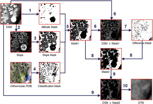
For the treatment, the following initial premises have been established: (1) Value of Z in cells which do not have a significant influence of the vegetation must be unchanged. (2) Cells in which the Z value is determined by vegetation are cancelled and incorporated into the vegetation mask. (3) Identification and isolation of cells influenced by vegetation is done by a combination of geometric and spectral criteria and (4) The final product must be obtained by filling the cells attributed to the vegetation using a procedure that takes into account the Z values of the edge of the surrounding area of the gap without producing any change in the rest of cells.

Once the final DTM was obtained, the quality of the DTM was controlled in the areas occupied by vegetation, for which information related to 30 additional verification points, obtained in the field, was used.

Finally, once the DTM has been obtained, GIS queries have been made to determine the volumes between the surface defined by the DTM and horizontal planes at different levels. This has allowed the elaboration of a filling curve that relates the water level with the volume stored by the pond. At the same time, the surface (number of cells x surface of each cell) that is below each flood level has been discriminated from the DTM histogram.

Results and discussion

For each flight, three cartographic products were obtained whose characteristics are indicated in Table 3.

Table 3. Characteristics of the cartographic products obtained in each flight.

	FV-8	Phantom
Point cloud Number of 3D points Average density (per m^2)	56,476,969 423.68	13,611,503 95.39
Digital surface model (DSM) Resolution (cm/pixel) File size	6.90 122.8 MB 5403 x 5960	13.36 39.7 MB 3054 x 3410
Digital terrain model (DTM) Resolution (cm/pixel) File size	6.90 122.8 MB 5403 x 5960	16.7 25.4 MB 2443 x 2728
Orthomosaic Resolution (cm/pixel) File size	1.38 2.25 GB 27,013 x 29,800	3.34 476.7 MB 12,216 x 13,640

As indicated above, the DTM obtained in both flights has been directly discarded for its inadequate quality by showing clear evidence that the effect of shrub vegetation has not been removed from the model. The quality control performed by the checkpoints on the products obtained gives different results. Since flight altitude, environmental conditions and data processing have been similar, the differences are clearly due to the characteristics and quality of the camera used by each system.

The planimetric quality of the higher resolution orthomosaic, obtained by the FV-8 system, has been analyzed. Its positional quality is defined by a root mean-squared error in the X-coordinate (RMSE_X) of 0.025 m, an RMSE_Y of 0.029 m and an RMSE_XY of 0.038 m. These values can be considered excellent, especially when considering that a limitation to locate the checkpoints in the orthomosaic is the own size of the pixel (0.0138 m) that introduces certain indetermination in the location of the checkpoint in the image.

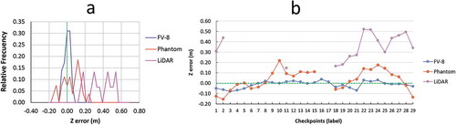
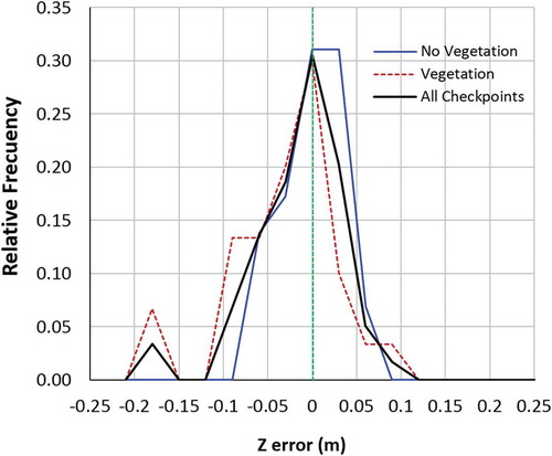
Using Z-coordinate of the checkpoints, the altimetric quality of the DSMs generated with both systems has been evaluated and compared with the official DTM (PNOA) obtained by LiDAR procedures. Figure 8(a) shows the frequency distribution of the errors in Z for the three models considered in this work. Error in Z is the difference between the Z obtained by differential GNSS and the value of the cell that occupies the planimetric position of the point in the model. Figure 8(b) shows the Z error of each of the checkpoints, according to the field measurement sequence. For the DSM obtained with the FV-8 system, the dispersion of the altimetric error is less than 3 cm in 48% of the points and less than 6 cm in 93% of the points. The RMSE_Z for this product turns out to be 0.035 m. For the DSM obtained with the Phantom system, a greater dispersion is observed with respect to the real values and a tendency for the Z-coordinate to be underestimated: 35% of the points have differences lower than 6 cm, 57% of the points present differences of less than 12 cm and 93% of less than 18 cm. The RMSE_Z for the set of points is 0.102 m in the model generated with the Phantom system, three times higher than the one obtained with the FV-8. As far as the PNOA-LiDAR product is concerned, the differences between the actual values and those obtained from the model are much higher, as they are always lower than the real value: 20% of the points have differences lower than 20 cm, 53% of the points present differences of less than 40 cm and 87% lower than 50 cm. In this case the RMSE_Z is 0.37 m.

Figure 8. (a) Frequency distribution of the error in Z for the DSM obtained with the FV-8 system, the phantom system and the official cartography obtained by LiDAR procedures. (b) Errors in Z of the 29 checkpoints for each of the cartographic products considered in this work.

Figure 9 shows the altimetric difference between the two DSMs generated in this work. It is observed that the differences between the two are between ±0.20 m (green, light blue, dark blue and yellow colors) for the range of altitudes corresponding to the terrain that constitutes the basin of the pond.

Figure 9. Altimetric differences in the two DMS obtained with the FV-8 and phantom systems. Figures in legend represent meters.

The results obtained from the DSM/FV-8 by the procedure applied to remove vegetation according to the scheme shown in Figure 6 are presented in Figure 10. It should be noted that in recent years precipitation has been very low thus resulting in very scarce flooding events in the area. Consequently, as it is deduced from the official orthophotographs of successive years, the pond has been gradually colonized by shrub vegetation, that in certain sectors reaches a high density and prevents the observation of the surface from above. This fact is undoubtedly an obstacle to the photogrammetric method. Thus, the surface of vegetation mask generated represents about 50% of the total land covered by the ortophotography. This requires the interpolation of a large number of data. However, if the sector without data is not too large and is surrounded or contains cells with data inside, the spline interpolation method (Schweikert, 1966) adjusts a surface that resembles the actual surface of the terrain.

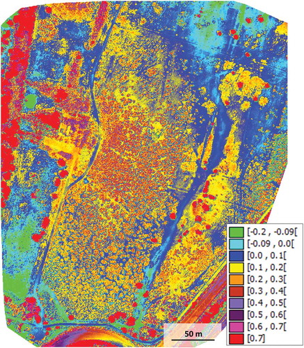
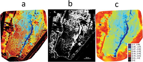
Figure 10. (a) Digital surface model (DSM), (b) vegetation mask with black color in cells with presence of vegetation and white color in cells with absence of vegetation and (c) digital terrain model (DTM). DTM and DSM are represented with the same color scheme. Figures in legend represent meters above sea level.

Using Z-coordinate of the checkpoints located on the vegetation, the altimetric quality of the interpolated DTM/FV-8 has been evaluated. Figure 11 shows the frequency distribution of the errors in Z for the checkpoints located within the vegetation compared with the errors in Z for the checkpoints located in areas without vegetation. A greater dispersion can be appreciated in the first set, although the maximum frequency is also very close to zero, resulting an RMSE_Z of 0.075 m, evidencing the goodness of the method used.

Figure 11. Frequency distribution of the error in Z for the DTM obtained with the FV-8 system, considering the control points in areas without vegetation (29 points) and in areas with vegetation (30 points) filled by the interpolation algorithm. The distribution of frequencies for all the points is also included.

In Figure 12, the DTM-LiDAR (PNOA) and the DTM generated after removal of vegetation from the DSM/FV-8 are compared with the same color scheme. First, a significant reduction in the size of the cell produced in this work (0.069 m vs. 5 m) can be observed, which leads to a significant improvement in the degree of detail of the terrain morphology. Second, it is observed that the official cartography systematically presents lower values of elevation (around 0.4 m), which shows a systematic error that can have significance when this document is used to evaluate, for example, the phenomena of flood and coastal risks. Although this value complies with the technical specifications of the product (RMSE_Z < 0.5 m), the existence of such a high bias is noticeable and requires an explanation. The existence of systematic errors in LiDAR altimetry data has been revealed by different authors, who have quantified and proposed correction methods (Filin, 2001; Schmid, Hadley, & Wijekoon, 2011). In general, values of less than 0.2 m are expected, although they depend closely on the type of cover and the filtering algorithms (Hladik & Alber, 2012; Huising & Gomes Pereira, 1998). In addition to the aspects related to calibration of the LIDAR system (both laboratory and in-fight), the type and density of vegetation and the presence of humidity increase systematic errors. Further, Crespo and Manso (2014) identify systematic errors in altitude of PNOA-LIDAR products up to 0.4 m related either to the orientation of the flight with respect to the orography, or to certain types of land covers. In any case, in order to verify the bias of the LiDAR data, a quality check has been made in this study. Five points belonging to the official high-precision leveling network (IGN, 2018) in the surrounded area have been considered. The results of the analysis support the existence of the detected systematic error.

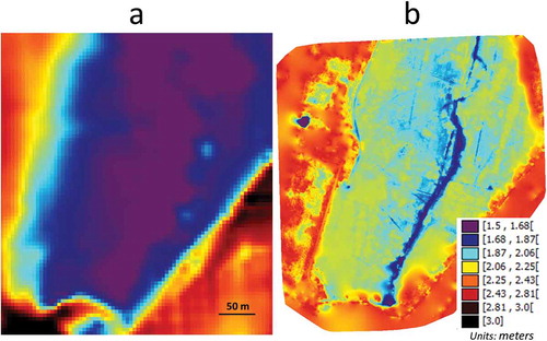
Figure 12. Comparison of DTM-LiDAR (PNOA) (a) and DTM-FV8 (b). Note: both are represented with the same color table. Figures in legend represent meters above sea level.

Therefore, it is inferred that the model generated by the FV-8 system presents a greater accuracy, which is an order of magnitude better than the one of the preexisting cartographic document (PNOA-LiDAR). The model generated by the Phantom system presents an intermediate accuracy between the two previous ones. It is for this reason that the model obtained with the FV-8 has been selected to produce the necessary data for the hydrological application proposed in this work.

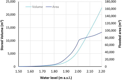
Finally, from the DTM by GIS analysis, the surfaces and volumes related to the different flood levels have been obtained, which have been used in the elaboration of the wetland stored volume/area flooded vs. water level graph (Figure 13). The evolution of the stored volume as a function of the increase of level of flood in the pond presents two linear sections. The first, which presents a smooth slope corresponds to flood levels below 1.85 m and is related to the filling of the central sulcus. The second section, with a much higher slope, extends from the 2 m flood level. This level corresponds to the maximum flood level of the lagoon in wet years. As for the evolution of the flooded area due to the increase in flood level, a sharp change is also observed around 2 m, indicating a change in the morphology of the bottom of the lagoon, with a notable increase in the slope of the basin in the edges.

Figure 13. Relationship between the volume stored/area of water sheet vs. water level in the pond.

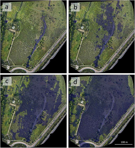
Figure 14 shows the simulation of the water sheet produced with different flood levels of the lagoon. The utility for the determination of the water budget in the wetland area is clear: if a daily control of the level of the lagoon is made, it is possible to determine the daily variations of stored volume and to relate these changes of storage with the rest of the elements of the balance. For example, after a rainy episode, the increase in volume stored in the pond can be related to the surface runoff generated on the basin, if the aquifer levels are below the lagoon, and thus the coefficient of runoff can be determined. In addition, by knowing the rate of evaporation (amount of evaporated water per unit area and time), the volume transferred to the atmosphere can be determined by the product of the flooded surface multiplied by the rate of evaporation and thereby reducing an unknown term of the water budget.

Figure 14. Flooded areas when the water level of the pond is 1.80, 1.90, 2.00 and 2.20 m from the mean sea level (general altimetric datum).

Conclusion

In this study, we show the applicability and the advantages of using UAV to generate very high resolution DTM to be used in the estimation of the water budget in a wetland area. The use of this technique allows the definition of the geometry of the pond with a degree of detail higher than that of the preexisting cartographic products. Therefore, this method may be used to predict volumes of stored water from the control of elevation of the flood. In addition, the estimation of the surface of the water sheet based on the measurement of the water level facilitates the estimation of the different elements of the water budget as, for example, the direct evaporation from the wetland or the addition of water from rainfall.

The orthomosaic performed with the higher resolution camera (Sony Alfa-7) offers a 1.4 cm of cell size and an RMSE in planimetry of 3.8 cm. The DTM generated with a cell size of 6.9 cm presents an RMS in the Z-coordinate of 3.5 cm, which is three times lower than that obtained by the lower performance DJI Phantom system. This is basically attributed to the characteristics of the camera. In addition, the detail of the model is one order of magnitude higher than that obtained for the official cartographic DTM-PNOA (LiDAR).

The main disadvantage of the methodology used is related to the presence of vegetation, which, unlike LiDAR techniques, prevents the capture of terrain data under the vegetation cover and force the elimination of a significant part of recorded information. In order to filter the effect of the vegetation in the DSM, combined spectral and morphological techniques have been used. Threshold criteria have been used in the elevation and in the local slope. Then, a procedure to detect and eliminate discrepant cells with a higher elevation compared to an adjusted surface after a minimum filtering has been applied. The quality control carried out on the areas occupied by vegetation in the DTM provides an RMSE_Z of 7.5 cm, somewhat higher than that obtained in areas without vegetation, which support the methodology used. The global RMSE_Z for the DTM, including zones with and without vegetation, is estimated at 5.9 cm.

Future work for the isolation and minimization of effect of vegetation in the production of the DTM may include (1) perform the flight in season with less vegetation (late summer), (2) to minimize the effect of the shade by acquiring the images with zenital light and (3) combining RGB and multispectral images in order to perform a vegetation filtering by spectral characteristics.

Acknowledgments

The authors thank Jordi Corbera and anonymous reviewer for their appropriate and timely observations that have contributed to the improvement of the work.

Disclosure statement

No potential conflict of interest was reported by the authors.

Additional information

Funding

This work is supported by Proyecto de Infraestructuras MINECO-FEDER UNCA [grant number 2013-1E-1969].

References

- Adam, E., Mutanga, O., & Rugege, D. (2010). Multispectral and hyperspectral remote sensing for identification and mapping of wetland vegetation: A review. Wetlands Ecology and Management, 18, 281–296.
- Boon, M.A., Greenfield, R., & Tesfamichael, S. (2016). Unmanned aerial vehicle (UAV) photogrammetry produces accurate high-resolution orthophotos, point clouds and surface models for mapping wetlands. South African Journal of Geomatics, 5–2, 186–200.
- Chabot, D., & Bird, D.M. (2013). Small unmanned aircraft: Precise and convenient new tools for surveying wetlands. Journal of Unmanned Vehicles System, 1, 15–24.
- Chabot, D., Carignan, V., & Bird, D.M. (2014). Measuring habitat quality for least bitterns in a created wetland with use of a small unmanned aircraft. Wetlands, 34, 527–533..
- Crespo, M., & Manso, M.I. (2014) Control de calidad del vuelo Lidar utilizado para la modelización 3D de las fallas de Alhama (Murcia) y Carboneras (Almería) [Quality control of the Lidar flight used for the 3D modeling of the faults of Alhama (Murcia) and Carboneras (Almería)] Universidad Politécnica de Madrid, 125 pp. http://oa.upm.es/33673/1/PFC_MIGUEL_CRESPO_MAZO.pdf
- CSG, Consejo Superior Geográfico http://www.idee.es/web/guest/europeo-inspire. ( Accessed 17 06.2017)
- DeBell, L., Anderson, K., Brazier, R.E., King, N., & Jones, L. (2016). Water resource management at catchment scales using lightweight UAVs: Current capabilities and future perspectives. Journal of Unmanned Vehicles System, 4, 7–30.
- Filin, S. (2001). Recovery of systematic biases in laser altimeters using natural surfaces. International Archives of Photogrammetry and Remote Sensing, XXXIV-3/W4, 85–91.
- García de Lomas, J., García, C.M., & Canca, I. (2004). Caracterización y fenología de las lagunas temporales del Pinar de La Algaida (Puerto Real, Cádiz) [Characterization and phenology of the temporal gaps in the Pinar of Algaida (Puerto Real, Cádiz)]. Revista de la Sociedad Gaditana de Historia Natural, 4, 105–124.
- García-López, S., Ruiz-Ortiz, V., & Muñoz-Pérez, J.J. (2018). Time-lapse photography for monitoring reservoir leakages (Montejaque dam, Andalusia, southern Spain). Hydrology Research, 49(1), 281–290.
- García-López, S., Ruiz-Ortiz, V., Sánchez-Bellón, A., Barbero, L., Muñoz-Arroyo, G., Castro, M., & Rebordinos, L. (2016). Uso del humedal de Los Toruños (Puerto Real, Cádiz) como laboratorio natural para la enseñanza de Hidrogeología [Use of the “Los Toruños” wetland (Puerto Real, Cadiz) as a natural laboratory for teaching hydrogeology]. In:Giráldez Cervera, J.V., López Geta, J.A., Ramos González, G. & Roldán Cañas, J. (Eds): Jornada Hidrogeología y Humedales: 45 años del Convenio de Ramsar, 21, Universidad de Córdoba.
- Gilvear, D., & Bradley, C. (2000). Hydrological monitoring and surveillance for wetland conservation and management; a UK perspective. Physics and Chemistry of the Earth, Part B: Hydrology, Oceans and Atmosphere, 25(7–8), 571–588.
- Gutiérrez-Mas, J.M., & García-López, S. (2015). Recent evolution of the river mouth intertidal zone at the Río San Pedro tidal channel (Cádiz Bay, SW Spain): Controlling factors of geomorphologic and depositional changes. Geologica Acta, 13–2, 123–136.
- Hladik, C., & Alber, M. (2012). Accuracy assessment and correction of a LIDAR-derived salt marsh digital elevation model. Remote Sensing of Environment, 121(2012), 224–235.
- Huising, E.J., & Gomes Pereira, L.M. (1998). Errors and accuracy estimates of laser data acquired by various laser scanning systems for topographic applications. ISPRS Journal of Photogrammetry & Remote Sensing, 53(1998), 245–261.
- IGN, Instituto Geográfico Nacional. http://pnoa.ign.es ( Accessed 17 06 2017)
- IGN, Instituto Geográfico Nacional. http://www.ign.es/web/resources/geodesia/visorGeodesia/index.html ( Accessed 25 07 2018)
- Junta, D.A. Consejería de Medio Ambiente y Ordenación del Territorio. Parque Natural Bahía de Cádiz http://www.juntadeandalucia.es/medioambiente/site/portalweb/menuitem.f497978fb79f8c757163ed105510e1ca/?vgnextoid=3092545f021f4310VgnVCM1000001325e50aRCRD. ( Accessed 17 06 2017)
- Leitão, J.P., Moy de Vitry, M., Scheidegger, A., & Rieckermann, J. (2016). Assessing the quality of digital elevation models obtained from mini unmanned aerial vehicles for overland flow modelling in urban areas. Hydrology Earth System Sciences, 20, 1637–1653.
- Lejot, J., Delacourt, C., Piégay, H., Fournier, T., Trémélo, M.-L., & Allemand, P. (2007). Very high spatial resolution imagery for channel bathymetry and topography from an unmanned mapping controlled platform. Earth Surface Processes and Landforms, 32(11), 1705–1725.
- Madden, M., Jordan, T., Bernardes, S., Cotten, D.L., O’Hare, N., & Pasqua, A. (2015). Unmanned aerial systems and structure from motion revolutionize wetlands mapping. In: Tiner, R.W., Megan, W.L. & Klemas, V.V. (Eds) Remote Sensing of Wetlands: Applications and Advances. 195-219. CRC Press. ISBN 9781482237351.
- Maltby, E. (1991). Wetland management goals: Wise use and conservation. Landscape and Urban Planning, 20(1–3), 9–18.
- Mekiso, F.A., Ochieng, G.M., & Snyman, J. (2016). Water budget analysis for the middle mohlapitsi wetland in the oliphants river basin, Limpopo province, South Africa. International Journal of Environmental Engineering, 8(2–3), 179–199.
- Moral, F., Rodríguez-Rodríguez, M., Benavente, J., & Cifuentes, V. (2009). Lagunas de la Campiña Andaluza: Hidrogeología, modelo cuantitativo del hidroperiodo e implicaciones de la morfología de la cubeta en el funcionamiento hidrológico [Lakes of the Andalusian countryside: Hydrogeology, quantitative model of the hydroperiod and implications of the morphology of the bucket in the hydrological functioning]. La geología y la hidrogeología en la investigación de humedales”. Serie: Hidrogeología y Aguas Subterráneas. Instituto Geológico y Minero de España (Ed), Vol. 28, 45–65. ISBN 9788478407958.
- Nobajas, A., Waller, I.R., Robinson, Z.P., & Sanzongalo, R. (2017). Too much of a good thing? the role of detailed UAV imagery in characterizing large-scale badland drainage characteristics in South-Eastern Spain. International Journal of Remote Sensing, 2844–2860. doi:10.1080/01431161.2016.1274450
- Owen, C.R. (1995). Water budget and flow patterns in an urban Wetland. Journal of Hydrology, 169(1), 171–187.
- Pérez Hurtado, A., & García-Jiménez, C. ( coordinadores). (2004) Estudio de la adecuación y acondicionamiento para instalaciones y actuaciones de investigación y uso público de los terrenos colindantes al Río San Pedro, Puerto Real, Cádiz [Study of fitness and conditioning facilities and performance of research and public use of the land adjacent to the river San Pedro, Puerto Real, Cadiz]. Unpublished manuscript. 89 pp
- RAP, Red de Posicionamiento de Andalucía. http://www.ideandalucia.es/portal/web/portal-posicionamiento/rap. ( Accessed 17 06 2017)
- Richardson, C.J. (1994). Ecological functions and human values in wetlands: A framework for assessing forestry impacts. Wetlands, 14 1, 1–9. . Online.
- Schmid, K.A., Hadley, B.C., & Wijekoon, N. (2011). Vertical accuracy and use of topographic LiDAR data in coastal marshes. Journal of Coastal Research, 27(6A), 116–132.
- Schweikert, D.G. (1966). An interpolation curve using spline in tension. Journal of Mathematics and Physics, 45, 312–313.
- Serifoglu Yilmaz, C., & Gungor, O. (2016). Comparison of the performances of ground filtering algorithms and DTM generation from a UAV-based point cloud. Geocarto International, 1–16. doi:10.1080/10106049.2016.1265599
- Snavely, N., Seitz, S.N., & Szeliski, R. (2008). Modeling the world from internet photo collections. International Journal of Computer Vision, 80, 189–210.
- Tamminga, A.D., Eaton, B.C., & Hugenholtz, C.H. (2015). UAS-based remote sensing of fluvial change following an extreme flood event. Earth Surface Processes and Landforms, 40(11), 1464–1476.
- Vázquez-Tarrío, D., Borgniet, L., Liébault, F., & Recking, A. (2017). Using UAS optical imagery and SfM photogrammetry to characterize the surface grain size of gravel bars in a braided river (Vénéon River, French Alps). Geomorphology, 285, 94–105.
- Wang, Z., & Schenk, T. (2000). Building extraction and reconstruction from LiDAR data. International Archives of Photogrammetry and Remote Sensing, 33(B3/2; PART 3), 958–964.
- Westoby, M.J., Brasington, J., Glasser, N.F., Hambrey, M.J., & Reynolds, J.M. (2012). ‘Structure-from-Motion’ photogrammetry: A low-cost, effective tool for geoscience applications. Geomorphology, 179, 300–314.
- Wolf, B.M., & Heipke, C. (2007). Automatic extraction and delineation of single trees from remote sensing data. Machine Vision and Applications, 18, 317–330..
- Woodget, A.S., Austrums, R., Maddock, I.P., & Habit, E. (2017). Drones and digital photogrammetry: From classifications to continuums for monitoring river habitat and hydromorphology. Wiley Interdisciplinary Reviews: Water, 4(4). doi:10.1002/wat2.1222
- Xie, Y., Sha, Z., & Yu, M. (2008). Remote sensing imagery in vegetation mapping: A review. Journal of Plant Ecology, 1(1), 9–23.
- Zazo, S., Molina, J.L., & Rodríguez-Gonzálvez, P. (2015). Analysis of flood modeling through innovative geomatic methods. Journal of Hydrology, 524, 522–537.
- Zheng, L., Zhang, J., & Wang, Q. (2009). Mean-shift-based color segmentation of images containing green vegetation. Computers and Electronics in Agriculture, 65(1), 93–98.