A change detection framework by fusing threshold and clustering methods for optical medium resolution remote sensing images

ABSTRACT

In change detection (CD) of medium-resolution remote sensing images, the threshold and clustering methods are two kinds of the most popular ones. It is found that the threshold method of the expectation maximization (EM) algorithm usually generates a CD map including many false alarms but almost detecting all changes, and the fuzzy local information c-means algorithm (FLICM) obtains a homogenous CD map but with some missed detections. Therefore, a framework is designed to improve CD results by fusing the advantages of the threshold and clustering methods. The CD map generated by the clustering method of FLICM is used to remove false alarms in the CD map obtained by EM threshold method by an overlap fusion. Then, the local Markov random field model is implemented to verify the potentially missed detections. Finally, a fused CD map with less false alarms and missed detections is achieved. Two experiments were carried out on two Landsat ETM+ data sets. The proposed method obtained the least errors (1.11% and 3.51%) and the highest kappa coefficient (0.9366 and 0.8834), respectively, when compared with five popular CD methods.

KEYWORDS:

• Change detection
• remote sensing
• threshold
• clustering
• advantage fusion

Introduction

Change detection (CD) from remote sensing images identifies changes by analyzing multitemporal images acquired over the same geographical area at different times, such as land use/land cover, damages due to earthquakes, floods and fires, changes of roads, cities and plants (Chen, Moriya, Sakai, Koyama, & Cao, 2014; Lu, Mausel, Brondizio, & Moran, 2004; Mari, Laneve, Cadau, & Porcasi, 2012). In the past three decades, lots of CD methods have been proposed to automatically achieve accurate CD results (Hao, Shi, Zhang, & Li, 2014; Moser, Angiati, & Serpico, 2011). All methods can be grouped into supervised and unsupervised types. The former detects changes and supply change types by comparing the classification maps of bitemporal images. However, it needs the ground reference, which limits its application. The latter identifies changes without needing the ground reference; therefore, the study in this paper focuses on the unsupervised ones.

Three steps are usually involved in CD: (1) pre-processing, (2) image comparison and (3) image analysis. In the first step, several corrections need implementing between bitemporal images to reduce the effects of light and atmospheric condition, such as co-registration, radiometric corrections (Mishra, Ghosh, & Ghosh, 2012; Ye & Shan, 2014). In the second step, the difference image is generated by pixel-by-pixel comparing between bitemporal images. Many methods have been used to generate the difference image, including the image differencing, image ratio, image correlation, image regression, log ratio for synthetic aperture radar (SAR) images and change vector analysis (CVA) (Shi, Shao, Hao, He, & Wang, 2016). In the third step, the difference image is analyzed and divided into changed and unchanged parts. In the beginning, visual analysis was applied to detect changes, which costs much time and limits the production efficiency (Leichtle, Geiss, Wurm, Lakes, & Taubenboeck, 2017). Afterward, a trial-and-error threshold method was implemented by changing the threshold value, and an empirical threshold method was developed to identify changes using $x_i>m+T\cdot \sigma$, where $x_i$ is the grey value of the ith pixel, T is a constant, $m$ and $\sigma$ are the mean and standard deviation of the difference image, respectively (Fung & LeDrew, 1988). In order to improve the efficiency, some automatic threshold methods were proposed (Bazi, Bruzzone, & Melgani, 2005; Im, Jensen, & Hodgson, 2008). One of the most popular threshold methods was proposed by Bruzzone and Prieto (2000), where the difference image is supposed as mixture Gaussian model and the Bayes rule for minimum error is adopted to calculate the threshold using expectation maximization (EM) algorithm. Due to much false alarms existing in the change map obtained by threshold, the spatial information was introduced by some advanced models, such as Markov random model (Hao, Shi, Deng, & Zhang, 2014; Subudhi, Ghosh, Nanda, & Ghosh, 2017), support vector machine (Bovolo, Bruzzone, & Marconcini, 2008; Nemmour & Chibani, 2006), artificial neural network (Wang, Shi, Atkinson, & Li, 2015; Xu, Ricci, Yan, Song, & Sebe, 2015), wavelet transform (Celik & Ma, 2011; Li, Shi, Zhang, & Hao, 2017), active contour model (Hao, Shi, Zhang, et al., 2014; Li, Gong, & Liu, 2015), and fuzzy c-means clustering (FCM) algorithm (Ghosh, Mishra, & Ghosh, 2011; Krinidis & Chatzis, 2010; Mishra et al., 2012). The ranges of pixel grey values in the difference image belonging to the changed and unchanged clusters often have an overlap, and FCM has robust characteristics for ambiguity and provides an appropriate choice to identify them by using fuzzy set information (Ghosh et al., 2011). The improved ones mainly contain an improved local energy term of exploiting spatial information, where a robust fuzzy local information c-means (FLICM) was proposed by Krinidis and Chatzis (2010) for image segmentation. A novel fuzzy factor was added into FCM to guarantee noise insensitiveness, which usually smoothed detailed changes due to overuse of spatial information (Zhang, Wang, Shi, & Hao, 2017).

It is found that the threshold method, i.e. the EM algorithm, usually generates more false alarms but less missed detections than the clustering algorithm, such as active contour model and FLICM. The EM threshold method generates a CD map including many false alarms but almost detecting all changes. FLICM obtains a CD map including fewer false alarms (Hao, Zhang, Li, & Chen, 2017). Therefore, we aim to design a framework to improve CD results by fusing the advantages of threshold and clustering methods.

Methodology

Let X₁ and X₂ be two multispectral images acquired from the same geographical area at two different times. Assuming images have been co-registered and radiometrically corrected, the two images have the same size of M × N. The designed framework mainly includes three parts as shown in Figure 1. First, the difference image X is generated by the magnitude of CVA or image differencing, and consists of changed pixels W₁ and unchanged pixels W₂. Second, EM threshold and FLICM CD methods are implemented to the difference image and two initial CD maps are yielded. Then, an advantage fusion strategy is proposed to fuse two initial CD maps by taking full use of their advantages and obtain the final CD map.

Figure 1. Flowchart of the designed framework

EM threshold method

In this study, it is assumed that the difference image X can be seen as a Gaussian mixture, as follows:

(1) $p(X)=p(X/W_1)P(W_1)+p(X/W_2)P(W_2)$(1)

where p(X), p(X/W₁) and p(X/W₂) are the probability density functions of the difference image X, changed pixels W₁ and unchanged pixels W₂, and P(W₁) and P(W₂) are the a priori probabilities of changed pixels and unchanged pixels, respectively. The probability density functions p(X/W₁) and p(X/W₂) are Gaussian and can be written as follows:

(2) $p\left(X/W_k\right)=\frac{1}{{\sigma }_k\sqrt{2\pi }}exp\left[-\frac{{(X-{\mu }_k)}^2}{2{\sigma }_k^2}\right]$(2)

where $k\in (1,2)$, ${\mu }_k$ and ${\sigma }_k$ are the respective mean and variance of the corresponding pixels of class W_k.

EM can be performed to estimate the mean values ${\mu }_k$ by the following three steps (Hao, Shi, Zhang, et al., 2014).

Step 1: Initialize the means ${\mu }_k$, covariance ${\sigma }_k$ and a priori probability P(W_k). A threshold d to the difference image was set to obtain the initial changed pixels and unchanged pixels. The threshold can be generated from an empirical equation written as follows:

(3) $d={\mu }_{\mathrm{X}}+R\cdot {\sigma }_{\mathrm{X}}$(3)

where R is a constant, ${\mu }_{\mathrm{X}}$ and ${\sigma }_{\mathrm{X}}$ denote the respective mean and standard deviation of the difference image. The values of ${\mu }_k$, ${\sigma }_k$ and P(W_k) can then be computed from the classified pixels and regarded as the initial values to EM.

Step 2: Expectation step. The a posterior probability P(W_k/X) was evaluated as follows:

(4) $P(W_k/x_i)=\frac{P(W_k)p(x_i/W_k)}{P(x_i)}$(4)

where $1\le i\le MN$ and x_i is the ith pixel of the difference image.

Step 3: Maximization step. Re-estimate the parameters using the following equations:

(5) $P^{t+1}(W_k)=\frac{\sum _{i=1}^{MN}P{}^t(W_k/x_i)}{MN}$(5)

(6) ${\mu }_k^{{ }^{t+1}}=\frac{\sum _{i=1}^{MN}P{}^t(W_k/x_i)x_i}{\sum _{i=1}^{MN}P{}^t(W_k/x_i)}$(6)

(7) $({\sigma }_k^{{ }^2}{)}^{t+1}=\frac{\sum _{i=1}^{MN}P{}^t(W_k/x_i){(x_i-{\mu }_k)}^2}{\sum _{i=1}^{MN}P{}^t(W_k/x_i)}$(7)

where the superscripts t and t + 1 are the current and next iterations, respectively.

The parameters are estimated by the steps above and then checked for convergence. If the convergence criterion is not satisfied, repeat steps 2 and 3 until convergence is achieved. Finally, the mean values are estimated.

Finally, the Bayes rule for minimum error is adopted to calculate the threshold T₀ according to the following equation:

(8) $\left({\sigma }_2^2-{\sigma }_1^2\right){T_0}^2+2\left({\mu }_2{\sigma }_1^2-{\mu }_1{\sigma }_2^2\right){T_0}^2+{\mu }_1^2{\sigma }_2^2-{\mu }_2^2{\sigma }_1^2-2{\sigma }_2^2{\sigma }_1^{2}ln\left[\frac{{\sigma }_{1}P\left({\omega }_2\right)}{{\sigma }_{2}P\left({\omega }_1\right)}\right]=0$(8)

FLICM-based clustering method

Dunn (1973) first developed FCM algorithm and later extended by Bezdek (1981). This clustering algorithm aims at producing and optimal c partition through an iterative clustering process. Suppose there are N pixels in the difference image $\mathbf{X}=\left\{x_1,x_2,\cdots ,x_N\right\}$, and c is the number of the clusters. The FCM aims at obtaining membership probability $u_{ki}\in \left[0,1\right]$ $\left(\sum _{k=1}^c{u}_{ki}=1\left(i=\right.\right.$ $1,2,\cdots ,N))$ of the pixel x_i in the difference image for the kth cluster by minimizing the objective function as follows:

(9) $J_m=\sum _{i=1}^N\sum _{k=1}^c{u}_{ki}^m{∥x_i-v_k∥}^2$(9)

where $u_{ki}$ is the degree of membership value of pixel $x_i$ in the kth cluster, $v_k$ is the prototype of the center of cluster k, m is the weighing exponent in each fuzzy membership, and ${∥x_i-v_k∥}^2$ is the Euclidean distance between object x_i and the cluster center $v_k$.

To improve the robustness of the conventional FCM, local information has been introduced to extend it. Krinidis and Chatzis (2010) proposed a robust FLICM clustering algorithm to overcome the disadvantages of the absence of spatial information in the initial FCM algorithm. A fuzzy local similarity measure factor G was added into FCM, aiming to guarantee noise insensitiveness and image detail preservation (Krinidis & Chatzis, 2010), and the modified object function is written as follows:

(10) $J_m=\sum _{i=1}^N\sum _{k=1}^c\left[u_{ki}^m{∥x_i-v_k∥}^2+G_{ki}\right]$(10)

where the $x_i$ is the gray value of the ith pixel, N is the number of pixels in the difference image, $v_k$ is the prototype of the center of cluster k, $u_{ki}$ denotes the fuzzy membership of the i-th pixel with respect to cluster k, and for each pixel $x_i$, the fuzzy membership satisfies the constraint that $\sum _{k=1}^c{u}_{ki}=1$. Additionally, the added local factor is defined as follows:

(11) $G_{ki}=\sum _{j\in N_i}\frac{1}{d_{ij}+1}{\left(1-u_{kj}\right)}^m{∥x_j-v_k∥}^2$(11)

where the ith pixel is the center of the local window, the jth pixel represents the neighborhood pixels within the currently local window of the ith pixel, and d_ij is the spatial Euclidean distance between pixels i and j. $u_{kj}$ denotes the fuzzy membership of the gray value j in terms of the k-th cluster, and $v_k$ represents the prototype of the center of cluster k.

Fusion of two kinds of method

In order to take full use of the advantages of threshold and clustering CD methods, a fusion strategy is designed to remove noise and retain detailed changes. As for CD methods incorporating contextual information, they usually miss changes around edges because of the overused contextual information, such as FLICM. The EM threshold method can detect almost all changes and obtain accurate shapes of changed regions. Therefore, the CD map generated by FLICM is adopted to refine the one obtained by EM threshold method using an overlap fusion and local Markov random field (LMRF). The flowchart of the proposed fusion strategy is shown in Figure 2, and the details can be found as follows.

Figure 2. Flowchart of the spatial advantage fusion strategy

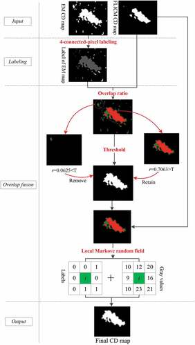
Step 1: Labelling the EM CD map. For the EM CD map, the independent changed regions are labelled as clusters $C=\left\{C_i,1\le i\le n\right\}$ for the connected components with four-connected pixels, labelled from 1 to n, as shown in Figure 2.

Step 2: Overlap fusion. For the labelled cluster C_i, the overlap ratio r_i is calculated referencing the FLICM CD map using $r_i=n_1/n_2$, where n₁ is the pixel number in C_i and n₂ is the number of changed pixels in the corresponding region of FLICM CD map. Set a threshold T to the overlap ratio r_i. If r_i > T, the cluster C_i is remained as changes; in contrary, it is removed as false alarms. Therefore, an initial fusion CD map can be produced after this step.

Step 3: LMRF fusion. Compared with the initially fused CD map in the step 2, the potentially missed (no-overlap) pixels in FLICM CD map are detected (e.g. green pixels shown in LMRF fusion part of Figure 2). For all potentially missed pixels, LMRF is designed to the identified missed pixels by minimizing the following energy function $U(x_i)$ with a pixel x_i

(12) $U(x_i)=\left(1-\beta \right)U_{\mathrm{s}}(x_i)+\beta U_{\mathrm{c}}(x_i)$(12)

where $\beta >0$ is a parameter with value fixed by the user to tuning the weight of spatial information, U_s (x_i) describes the spectral energy function from the difference image, and U_c(x_i) represents the energy term of contextual information computed from the local neighborhood N_i of the center pixel x_i. In the process of calculation, the U_s (x_i) and U_c(x_i) are normalized respectively.

The detailed spectral energy term can be written as follows:

(13) $U_{\mathrm{s}}(x_i)=\frac{1}{2}ln\left|2\pi {\sigma }_k^2\right|+\frac{1}{2}(x_i-{\mu }_k{)}^2({\sigma }_k^2{)}^{-1}$(13)

where ${\mu }_k$ and ${\sigma }_k^2$ denote the mean and variance of class k, respectively, that can be calculated from the initial change map generated by FLICM.

The spatial energy of the pixel x_i is defined as follows:

(14) $U_{\mathrm{s}\mathrm{p}\mathrm{a}\mathrm{t}\mathrm{i}\mathrm{a}\mathrm{l}}(x_i)=\sum _{j\in {\mathrm{N}}_i}I(l(x_i),l(x_j))$(14)

where N_i denotes the local neighborhood of the pixel x_i ($i\notin {\mathrm{N}}_i$), l(x_i) and l(x_j) ($j\in {\mathrm{N}}_i$) represent the class label of the pixel x_i and its local neighborhood, and the function I is defined as follows:

(15) $I(l(x_i),l(x_j))=\left\{\begin{array}{c}-1l(x_i)=l(x_j)\\ 0l(x_i)\ne l(x_j)\end{array}\right.$(15)

Step 4: Output. The potentially missed pixels are relabeled by minimizing the energy of LMRF, and other pixels keep the original labels in the initially fused CD map.

Experimental results

In order to evaluate the effectiveness of the proposed method, several experiments were carried out on two remote sensing data sets. Additionally, five popular methods were implemented as a comparison, including EM threshold, fusion of EM and Markov random field (EMMRF), FLICM, superpixel-based active contour model (SACM) (Hao, Shi, Deng, & Feng, 2016), and undecimated discrete wavelet transform and active contour (UDWTAC) (Celik & Ma, 2011). All the experiments were implemented using Matlab 8.4 on a personal computer with 2.2 GHz CPU and 8.00 GB RAM. Four indices are used to quantitatively assess the results as follows. (1) Missed detections N_m that indicate the number of actually changed pixels that were incorrectly classified as unchanged ones in the CD map. The ratio of missed detections P_m is calculated by $P_{\mathrm{m}}=N_{\mathrm{m}}/N_0\times 100\mathrm{\%}$, where N₀ is the total number of changed pixels counted in the ground reference map; (2) False alarms N_f indicate the number of actually unchanged pixels that were incorrectly determined as changed ones in the CD map. The ratio of false alarms P_f is calculated with the ratio $P_{\mathrm{f}}=N_{\mathrm{f}}/N_1\times 100\mathrm{\%}$, where N₁ is the total number of unchanged pixels counted in the ground reference map; (3) Total errors N_t indicate the total number of detection errors, including both missed and false detections. This total number refers to the sum of missed detections and false alarms. Hence, the ratio of total errors P_t is calculated with $P_{\mathrm{t}}=(N_{\mathrm{m}}+N_{\mathrm{f}})/(N_0+N_1)\times 100\mathrm{\%}$; and (4) Kappa coefficient $\kappa$.

Experiments of data set 1

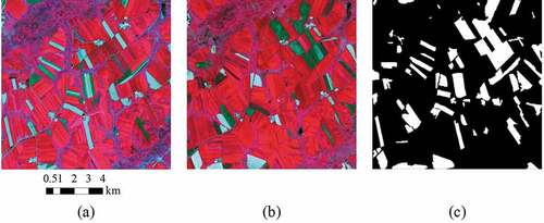
The first data sets used in experiments are two images acquired by the Landsat Enhanced Thematic Mapper Plus (ETM+) sensor of the Landsat-7 satellite in an area of Mexico in April 2000 and May 2002, and a section of 512 × 512 pixels was selected as test site. Image X₁ was registered to image X₂ using the linear transformation model, and the relative radiometric correction was implemented using the histogram-matching method (Coltuc, Bolon, & Chassery, 2006) by referencing image X₂. The value of root mean square error on the geometric correction was 0.7. The changes were caused by a fire that burned a large part of the vegetation in the test region. Figure 3(a,b) show the band 4 of 2000 and 2002 images, respectively. The image differencing method was implemented to the band 4 of bi-temporal images to generate the difference image. A reference map was manually obtained by a detailed visual analysis of both the available multitemporal images and the difference image as shown in Figure 3(c).

Figure 3. Band 4 of the data set 1 acquired in (a) April 2000 and (b) May 2002, and (c) is the ground reference map

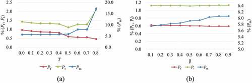
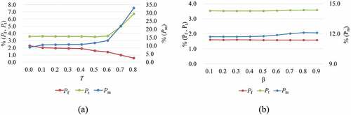
In the proposed approach, the overlap threshold T and the weight parameter β of contextual information affect the CD accuracy. Figure 4(a) shows the change patterns of the CD accuracy indices with the changing threshold T, where the weight parameter was set to 0.5 and the threshold ranged from 0 to 0.8 with the steps 0.1. It can be seen that the ratios of missed detection and total errors go down until the threshold value of 0.5, then increase. The ratio of false alarms always decreases with the increasing threshold. Figure 4(b) shows the change patterns of the accuracy indices with the weight parameter β ranging from 0.1 to 0.9 with the steps 0.1, in which the threshold T was set to 0.5. The ratio of missed detections has a slight increase, and the ratio of false alarms has a slight decrease with the increasing weight parameter. But the ratio of total errors almost keeps stable with the increase of the weight parameter.

Figure 4. Change patterns of the CD accuracy indices with (a) the ranging threshold T and (b) the changing weight parameter β for the data set 1

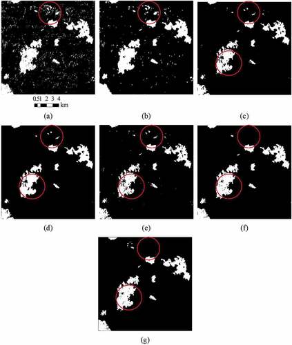
Figure 5 shows the CD maps obtained by EM, EMMRF, FLICM and the proposed method, respectively. The weight parameter $\beta$ in EMMRF controls the effect of spatial information, and a larger weight obtains a smoother CD map. It was set to 0.4 in this study. The segment scale Q determines the superpixel scale and the contour length μ controls the smooth of CD map in SACM. They were set to 128 and 0.2, respectively. The contour length μ in UDWTAC was set to 0.1. All values of parameters in the above contrast experiments were manually set to obtain highly accurate results. The overlap threshold T in the proposed method was set to 0.5 by referencing the accuracy change patterns under different overlap thresholds. As can be seen in Figure 5(a), the change map of EM contains almost all changes, but many false alarms exist at the same time (e.g. circle region). EMMRF gives homogenous regions by using spatial context, but much detailed information (e.g. accurate shapes of changed regions) is removed and lots of false alarms still exist as shown in the circle region of Figure 5(b). This is explained by the factor that it depends on the initial CD map of EM and neglects the fuzzy spatial information. In contrast, FLICM and SACM obtain more homogenous CD maps than EM due to incorporating local information, but it misses some detailed changes due to the overused spatial information. The CD map obtained by UDWTAC was displayed in Figure 5(e), which contains many false alarms as shown by circle regions. However, the proposed method can remove false alarms and retain details more efficiently as shown in the circle regions of Figure 5(f), which generates the most similar CD map to the ground reference among all the methods in this study. The reason is that the proposed method reduces the false alarms existing in the EM-based results by taking advantage of the FLICM CD map and retains detailed changes through the LMRF.

Figure 5. CD results of the data set Mexico obtained by (a) EM, (b) EMMRF, (c) FLICM, (d) SACM, (e) UDWTAC, (f) proposed method, and (g) is the ground reference map

Table 1 presents the accuracy comparisons of missed detections, false alarms, total errors and kappa coefficient among these methods. EM results in the maximum false alarms of 9792 pixels, and EMMRF generates the minimum missed detections of 796 pixels and false alarms of 5076 pixels, which reduces missed detections and false alarms compared with EM by incorporating fuzzy spatial information. For FLICM, it reduces much false alarms compared with EM due to the introduction of local information, where the total errors are 4947 pixels. SACM and UDWTAC generate similarly accurate CD maps with FLICM. It is worth noting the proposed method obtains the most accurate CD results among all methods used in this study via the total errors and kappa coefficient, and the missed detections, false alarms and total errors are 1512, 1410 and 2922, respectively. More importantly, it results in less missed detections than FLICM and much less false alarms than EM. Experimental results have indicated that the proposed method is insensitive to the overlap ratio and weight parameters. The EM method costs the least time of 1.1 s, and the FLICM method needs 12.8 s which costs much computation time than other comparative methods. The proposed method is a little slower than FLICM but slower than other four methods because it combines EM and FLICM.

Table 1. Quantitative CD results of the data set 1. P_m, P_f and P_t are ratios of missed detections, false alarms and total errors, respectively, and $\kappa$ represents the kappa coefficient

	Missed detections		False alarms		Total errors
Method	No. of pixels	$P_{\mathrm{m}}$	No. of pixels	$P_{\mathrm{f}}$	No. of pixels	$P_{\mathrm{t}}$	$\kappa$	Time (s)
EM	1329	5.19	9792	4.14	11,121	4.24	0.7901	1.1
EMMRF	796	3.11	5076	2.15	5872	2.24	0.8817	4.5
FLICM	4109	16.06	838	0.35	4947	1.89	0.8864	12.8
SACM	3900	15.24	891	0.38	4791	1.83	0.8915	6.7
UDWTAC	4021	15.71	987	0.42	5008	1.91	0.8855	9.0
Proposed	1512	5.91	1410	0.60	2922	1.11	0.9366	14.9

Experiments of data set 2

The second data set was acquired by Landsat-7 ETM+ sensor in August 2001 and August 2002 in the northeast region of China. A section (400 × 400 pixels) of the entire scene was selected as the test site. Figure 6(a,b) show the false color composite using the NIR band (R-4, G-3 and B-2), respectively. The image of 2001 was registered to the image of 2002 using the linear transformation model. The value of root mean square error on the geometric correction was 0.6. Then, the histogram-matching method was implemented to the former image for the relative radiometric correction by referencing the latter one. The difference image was generated by CVA based on all bands except for the thermal infrared band. A reference map was manually produced by a detailed visual analysis as shown in Figure 6(c).

Figure 6. False color composite (R-4, G-3 and B-2) of the data set 2 acquired in (a) August 2001, (b) August 2002, and (c) is the ground reference map

Figure 7(a) shows the change patterns of the CD accuracy indices with the increase of threshold T, in which the weight parameter was set to 0.5 and the threshold ranged from 0 to 0.8 with the steps 0.1. We can see that the ratio of false alarms always decreases with the increase of the threshold. As for the ratios of missed detections and total errors, they decline when the threshold ranges from 0 to 0.5, and then grow. As shown in Figure 7(b), different values of the weight parameter β have a slight influence on the accuracy indices. The ratio of missed detections slightly increases and the ratio of false alarms slightly decreases, respectively, with the increase of the weight parameter. But the ratio of total errors almost keeps stable.

Figure 7. Change patterns of the CD accuracy indices with (a) the increasing threshold T and (b) the changing weight parameter β for the data set 2

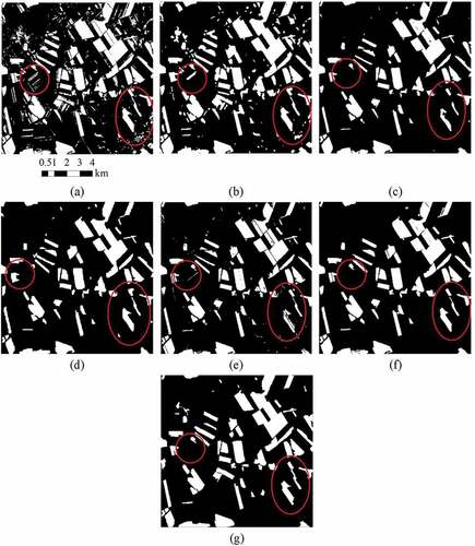
CD maps of the data set 2 are presented in Figure 8, which are generated by EM, EMMRF, FLICM and the proposed method, respectively. The value of parameter $\beta$ in EMMRF was set to 0.4, the segment scale Q and the μ value were set to 128 and 0.2, the μ value of UDWTAC was set to 0.1. All values of parameters in the above contrast experiments were manually set to obtain highly accurate results. The overlap threshold T in the proposed method was set to 0.5 by referencing the accuracy change patterns under different overlap thresholds. Figure 8(a) displays the change map produced by EM, which contains few missed detections but much false alarms (e.g. circle region). As can be seen from Figure 8(b), EMMRF generates a more homogenous change map than the one of EM, but lots of false alarms still exist and some regions are over smoothed. FLICM and SACM produce more homogenous CD maps than the above-mentioned methods because of using the fuzzy and local spatial information, respectively. But some detailed changes are missed due to the overused spatial information. The result obtained by UDWTAC has much noise as shown in Figure 8(e). The proposed method not only reduces the missed details as shown in Figure 8(f), but also yields a very homogenous CD map, which is the most similar one with the ground reference map.

Figure 8. CD results of data set farmland obtained by (a) EM, (b) EMMRF, (c) FLICM, (d) SACM, (e) UDWTAC, (f) proposed method, and (g) is the ground reference map

Table 2 displays the accuracy of the CD maps generated by the above-mentioned methods. EM generates few missed detections and the maximum false alarms. Though EMMRF reduces the missed detections of EM, it still contains many false alarms. FLICM generates more missed detections but much less false alarms than EM and EMMRF, which reduces the false alarms to 1224 pixels by incorporating fuzzy local information. SACM and UDWTAC produce CD maps indicating similar accuracy with FLICM. It is worth noting that the proposed method produces the most accurate CD map by referencing the total errors and kappa coefficient, where both the false alarms and missed detections are significantly reduced compared with other methods used in this study. In total, the experiments indicate the effectiveness of the proposed method that removes false alarms and preserves detailed changes. The threshold method EM is very fast, which only needs 1.0 s, and the FLICM costs 10.0 s. Because the proposed method generates more accurate by combining EM and FLICM, it needs more computing time than other methods used in this paper.

Table 2. Quantitative CD results for the data set 2. P_m, P_f, and P_t are ratios of missed detections, false alarms and total errors, respectively, and $\kappa$ represents the kappa coefficient

	Missed detections		False alarms		Total errors
Methods	No. of pixels	$P_{\mathrm{m}}$	No. of pixels	$P_{\mathrm{f}}$	No. of pixels	$P_{\mathrm{t}}$	$\kappa$	Time (s)
EM	2329	7.69	10,040	7.74	12,369	7.73	0.7706	1.0
EMMRF	1852	6.11	9110	7.02	10,962	6.85	0.7956	4.8
FLICM	5647	18.64	1224	0.94	6871	4.29	0.8518	10.0
SACM	4635	15.29	1686	1.30	6321	3.95	0.8646	4.1
UDWTAC	5327	17.58	1547	1.19	6874	4.30	0.8530	7.8
Proposed	3564	11.76	2055	1.58	5619	3.51	0.8834	11.5

Discussion

This paper presents a CD framework by fusing threshold and clustering methods for optical medium resolution remote sensing images. Automatic threshold algorithms usually generate a CD map containing almost all real changes but many false alarms. Clustering methods usually produce less false alarms but many missed detections. A fusion strategy consisting of overlap fusion and local Markov random field fusion was proposed to detect more real changes and fewer false alarms. The proposed framework was tested using two Landsat EMT+ data sets. In the first data set, the changes between two images were caused by a forest fire. In the second data set, different kinds of changes happened because of crop planting. It was shown that the proposed method can obtain more accurate CD maps compared with other five popular CD methods. Through the second experiments, the proposed framework also works well for regions with different kinds of changes.

The proposed method is influenced by the overlap threshold and the weight parameter $\beta$. Its total errors firstly decrease when the overlap threshold increases and begin to increase after the overlap threshold reaching around 0.5. The main reason is that the false alarms cannot be removed when the overlap threshold is small, because most detected changes are retained for a small overlap threshold. Much real changes will be removed under a large overlap threshold. Therefore, the proposed method produces an accurate result under the overlap threshold value around 0.5. As for the weight parameter β, the ratio of missed detections slightly increases and the ratio of false alarms slightly decreases with the increasing weight parameter, respectively. But the ratio of total errors almost keeps stable and reaches minimal values at the weight parameter value of 0.5. Given that, both the overlap threshold and the weight parameters are suggested to set to 0.5 in other studies.

The advantage of the proposed method is that it achieves a good trade-off between missed detections and false alarms. It reduced many false alarms compared with the EM threshold method and EMMRF, and missed detections were slightly increased. The proposed method reduced missed detections when compared with the popular CD methods incorporating spatial information, such as FLICM, SACM and UDWTAC. The proposed method usually generates more accurate CD maps considering the total errors, and achieves a better consistency with the ground map referencing the kappa coefficients. The disadvantage is that the proposed method needs more time than other used methods in this study. The threshold method EM is very fast, which costs about 1.0 s for both experiments. However, the FLICM incorporating spatial information costs much time, about 10.0 s. As for the proposed method, though it generates more accurate results, it needs more computation time than other methods because of by combining EM and FLICM. Hence, when we want to obtain more accurate results, it is better to use the proposed method. It is better to obtain the threshold method when the change maps need producing in a shorter time.

This method was developed for medium-resolution images. Therefore, it should work for other images having similar resolution with Landsat images, such as Sentinel-2. However, it cannot work well for very-high-resolution (VHR) images so far. More challenges are raised when VHR images are used as input data sources in CD, such as larger reflectance variability in each class and different acquisition characteristics (e.g. sensor viewing geometry and shadow effect). The increased variability often results in too many false changes, known as the “salt and pepper” effect in the pixel-based CD approaches (Hussain, Chen, Cheng, Wei, & Stanley, 2013). The object-based methods take an image object as the unit, which makes better use of texture, shape, and spatial relationships with neighboring objects than the pixel-based ones. In the future work, we will extend this method to superpixel or object level to test its effectiveness. In addition, the proposed method can be extended to CD maps obtained by other methods, where few missed detections and false alarms exist, respectively, such as some fine- and coarse-resolution CD results. In this study, only Landsat ETM+ data sets were used to assess the proposed method, therefore, the future work will be focused on the evaluation to other type data sets and methods.

Conclusion

A CD framework of fusing the threshold and clustering CD methods is proposed to remove false alarms and preserve detailed changes simultaneously. The CD map generated by the clustering method of FLICM is used to refine the one obtained by EM threshold method through the overlap fusion. Therefore, false alarms can be removed and some potentially missed detections are found. Then, LMRF is implemented to verify the potentially missed detections. Experiments were conducted on two Landsat EMT+ data sets to assess the performance of the proposed method. Compared with some popular methods (i.e. EM, EMMRF, FLICM, SACM, and UDWTAC), the proposed method achieves improvements in both accuracy and visual interpretation, and produces the most accurate change maps. Results indicate that the proposed method not only obtains more homogenous CD maps, but also preserves more detailed changes than other methods used in this paper. In total, the proposed method provides an effective and unsupervised CD method from remote sensing images.

Acknowledgments

The authors would like to thank the editors and reviewers whose suggestions have significantly improved this paper.

Disclosure statement

The authors reported no potential conflict of interest.

Additional information

Funding

This work was supported by the Natural Science Foundation of Jiangsu Province [grant number BK20160248]; the National Natural Science Foundation of China grant number [41701504]; and Fundamental Research Funds for the Central Universities [grant number 2015XKQY09].

References

- Bazi, Y., Bruzzone, L., & Melgani, F. (2005). An unsupervised approach based on the generalized Gaussian model to automatic change detection in multitemporal SAR images. IEEE Transactions on Geoscience and Remote Sensing, 43, 874–887. doi:10.1109/TGRS.2004.842441
- Bezdek, J.C. (1981). Pattern recognition with fuzzy objective function algorithms. Norwell, MA, USA: Kluwer Academic Publishers.
- Bovolo, F., Bruzzone, L., & Marconcini, M. (2008). A novel approach to unsupervised change detection based on a semisupervised SVM and a similarity measure. IEEE Transactions on Geoscience and Remote Sensing, 46, 2070–2082. doi:10.1109/TGRS.2008.916643
- Bruzzone, L., & Prieto, D.F. (2000). Automatic analysis of the difference image for unsupervised change detection. IEEE Transactions on Geoscience and Remote Sensing, 38, 1171–1182. doi:10.1109/36.843009
- Celik, T., & Ma, K.K. (2011). Multitemporal image change detection using undecimated discrete wavelet transform and active contours. IEEE Transactions on Geoscience and Remote Sensing, 49, 706–716. doi:10.1109/TGRS.2010.2066979
- Chen, W., Moriya, K., Sakai, T., Koyama, L., & Cao, C.X. (2014). Monitoring of post-fire forest recovery under different restoration modes based on time series Landsat data. European Journal of Remote Sensing, 47, 153–168. doi:10.5721/EuJRS20144710
- Coltuc, D., Bolon, P., & Chassery, J.-M. (2006). Exact histogram specification. IEEE Transactions on Image Processing, 15, 1143–1152.
- Dunn, J.C. (1973). A fuzzy relative of the ISODATA process and its use in detecting compact well-separated clusters. Journal of Cybernetics, 3, 32–57. doi:10.1080/01969727308546046
- Fung, T., & LeDrew, E. (1988). The determination of optimal threshold levels for change detection using various accuracy indices. Photogrammetric Engineering and Remote Sensing, 54, 1449–1454.
- Ghosh, A., Mishra, N.S., & Ghosh, S. (2011). Fuzzy clustering algorithms for unsupervised change detection in remote sensing images. Information Sciences, 181, 699–715. doi:10.1016/j.ins.2010.10.016
- Hao, M., Shi, W., Deng, K., & Feng, Q. (2016). Superpixel-based active contour model for unsupervised change detection from satellite images. International Journal of Remote Sensing, 37, 4276–4295. doi:10.1080/01431161.2016.1210838
- Hao, M., Shi, W., Deng, K., & Zhang, H. (2014). A contrast-sensitive Potts model custom-designed for change detection. European Journal of Remote Sensing, 47, 643–654. doi:10.5721/EuJRS20144736
- Hao, M., Shi, W.Z., Zhang, H., & Li, C. (2014). Unsupervised change detection with expectation-maximization-based level set. IEEE Geoscience and Remote Sensing Letters, 11, 210–214. doi:10.1109/LGRS.2013.2252879
- Hao, M., Zhang, H., Li, Z.X., & Chen, B.Q. (2017). Unsupervised change detection using a novel fuzzy C-means clustering simultaneously incorporating local and global information. Multimedia Tools and Applications, 76, 20081–20098. doi:10.1007/s11042-017-4354-1
- Hussain, M., Chen, D., Cheng, A., Wei, H., & Stanley, D. (2013). Change detection from remotely sensed images: From pixel-based to object-based approaches. ISPRS Journal of Photogrammetry and Remote Sensing, 80, 91–106. doi:10.1016/j.isprsjprs.2013.03.006
- Im, J.H., Jensen, J.R., & Hodgson, M.E. (2008). Optimizing the binary discriminant function in change detection applications. Remote Sensing of Environment, 112, 2761–2776. doi:10.1016/j.rse.2008.01.007
- Krinidis, S., & Chatzis, V. (2010). A robust fuzzy local information C-means clustering algorithm. IEEE Transactions on Image Processing, 19, 1328–1337. doi:10.1109/TIP.2010.2040763
- Leichtle, T., Geiss, C., Wurm, M., Lakes, T., & Taubenboeck, H. (2017). Unsupervised change detection in VHR remote sensing imagery – An object-based clustering approach in a dynamic urban environment. International Journal of Applied Earth Observation and Geoinformation, 54, 15–27. doi:10.1016/j.jag.2016.08.010
- Li, H., Gong, M., & Liu, J. (2015). A local statistical fuzzy active contour model for change detection. IEEE Geoscience and Remote Sensing Letters, 12, 582–586. doi:10.1109/LGRS.2014.2352264
- Li, Z., Shi, W., Zhang, H., & Hao, M. (2017). Change detection based on Gabor wavelet features for very high resolution remote sensing images. IEEE Geoscience and Remote Sensing Letters, 14, 783–787. doi:10.1109/LGRS.2017.2681198
- Lu, D., Mausel, P., Brondizio, E., & Moran, E. (2004). Change detection techniques. International Journal of Remote Sensing, 25, 2365–2401. doi:10.1080/0143116031000139863
- Mari, N., Laneve, G., Cadau, E., & Porcasi, X. (2012). Fire damage assessment in Sardinia: The use of ALOS/PALSAR data for post fire effects management. European Journal of Remote Sensing, 45, 233–241. doi:10.5721/EuJRS20124521
- Mishra, N.S., Ghosh, S., & Ghosh, A. (2012). Fuzzy clustering algorithms incorporating local information for change detection in remotely sensed images. Applied Soft Computing, 12, 2683–2692. doi:10.1016/j.asoc.2012.03.060
- Moser, G., Angiati, E., & Serpico, S.B. (2011). Multiscale unsupervised change detection on optical images by Markov random fields and wavelets. IEEE Geoscience and Remote Sensing Letters, 8, 725–729. doi:10.1109/LGRS.2010.2102333
- Nemmour, H., & Chibani, Y. (2006). Multiple support vector machines for land cover change detection: An application for mapping urban extensions. ISPRS Journal of Photogrammetry and Remote Sensing, 61, 125–133. doi:10.1016/j.isprsjprs.2006.09.004
- Shi, W., Shao, P., Hao, M., He, P., & Wang, J. (2016). Fuzzy topology–based method for unsupervised change detection. Remote Sensing Letters, 7, 81–90. doi:10.1080/2150704X.2015.1109155
- Subudhi, B.N., Ghosh, S., Nanda, P.K., & Ghosh, A. (2017). Moving object detection using spatio-temporal multilayer compound Markov random field and histogram thresholding based change detection. Multimedia Tools and Applications, 76, 13511–13543.
- Wang, Q., Shi, W., Atkinson, P.M., & Li, Z. (2015). Land cover change detection at subpixel resolution with a Hopfield neural network. IEEE Journal of Selected Topics in Applied Earth Observations and Remote Sensing, 8, 1339–1352.
- Xu, D., Ricci, E., Yan, Y., Song, J., & Sebe, N. (2015). Learning deep representations of appearance and motion for anomalous event detection. arXiv preprint arXiv:1510.01553.
- Ye, Y., & Shan, J. (2014). A local descriptor based registration method for multispectral remote sensing images with non-linear intensity differences. ISPRS Journal of Photogrammetry and Remote Sensing, 90, 83–95. doi:10.1016/j.isprsjprs.2014.01.009
- Zhang, H., Wang, Q., Shi, W., & Hao, M. (2017). A novel adaptive fuzzy local information C-means clustering algorithm for remotely sensed imagery classification. IEEE Transactions on Geoscience and Remote Sensing, 55, 5057–5068. doi:10.1109/TGRS.2017.2702061