SUSM: a scenario-based urban growth simulation model using remote sensing data

ABSTRACT

The introduction of the Foreign Direct Investment (FDI) policy in 1991 made India one of the fastest growing economies in the world. This has had a profound effect on India’s urbanization. The rapid urbanization of Indian cities poses a threat to natural and social environments, as expansion of the cities often outpaces the urban planning process. Thus, smart and strategic planning processes that use current and easily available datasets in combination with future urbanization scenarios are needed. To this end, we developed the scenario-based urban growth simulation model (SUSM), which can be used for impact analysis of different planning measures in both spatial and temporal contexts. SUSM uses remote sensing derived inputs, such as land use maps, slope, roads and centres of urban areas along with urban development scenarios. It uses logistic regression for calibration and a constrained stochastic cellular automaton for simulation of urban growth.

SUSM is tested in one of the fastest growing urban agglomerations of India: The Pune metropolis, which covers an area of 1642 km². SUSM is calibrated using urban growth maps derived from LANDSAT satellite images from 1992 to 2001. Subsequently, SUSM was used to simulate urban growth of Pune for 2013. A comparison of the SUSM simulation result with the actually measured urban growth derived from a LANDSAT 8 scene from 2013 is used to validate SUSM and to assess the effect of urban plans upon the growth of Pune. Our results show that: (i) SUSM is capable of predicting the location of future urbanization with an accuracy of 79% and a fuzzy kappa index of agreement 0.81; (ii) inclusion of official urban development plans as input for SUSM did not provide a better agreement with the observed growth; (iii) SUSM, parameterized with remote sensing data, can be used effectively to understand urban growth and assess the effects of alternative urban development plans in terms of the spatial expansion of cities.

KEYWORDS:

• Cellular automata
• development plan
• logistic regression
• SUSM
• urban growth
• urban planning

Introduction

Today, urban areas are home to more than 54% of the world’s population and are expected to shelter 60% by 2030 (United Nations, 2016). The share of developing countries in the world’s urban population is rapidly increasing in comparison with developed countries (Berry, 2008; United Nations, 2016). Thus, developing countries face many challenges of rapid urbanization (Butsch et al., 2017), such as biodiversity loss (Grimm, Grove, Pickett, & Redman, 2008), reduced green spaces (Ramachandra, Aithal, & Sowmyashree, 2014), increased fragmentation of land (Shrestha, York, Boone, & Zhang, 2012), decreased air and water quality (Borges, Dos Santos, Caldas, & Lapa, 2015; Mage et al., 1996), loss of fertile agriculture (Li, Zhou, & Ouyang, 2013) and alteration of natural drainage (Wagner et al., 2016). Rapid urban growth, unless managed efficiently, can lead to serious environmental degradation and socio-economic disparities (Sandamali, Kantakumar, & Sivanantharajah, 2018). Sustainable and planned urbanization has many positive effects such as better accessibility to education, health care, employment and culture (Aguayo, Wiegand, Azócar, Wiegand, & Vega, 2007). However, traditional urban planning procedures used in developing countries are often outpaced by the rapid actual development. Moreover, datasets used in urban planning are often outdated resulting in insufficient infrastructure, as well as haphazard and unsustainable urban development. Many planners inherently use static urban growth models and mathematical formulations to characterize urban growth patterns and trends of rapidly growing cities (Batty, 2012; Itami, 1994; Roy, 2009). As a result, development plans prepared using traditional urban planning often bear little resemblance to reality (Itami, 1994; Roy, 2009). As an example, Mahadevia and Joshi (2009, p. 3) stated that “the preparation of master plans in India has become a statutory exercise to allocate the urban space with false notations of comprehensiveness using positivist methodologies that freezes lands and makes them unavailable for development and by that declaring large parts of city as illegal and informal”. Thus, planning itself has come to be regarded as part of the problem rather than the solution (Batty, 2008; Mahadevia & Joshi, 2009; Roy, 2009).

Figure 1. SUSM model structure.

The problem of timeliness of appropriate data can be addressed in part by using remote sensing. Remote sensing datasets can be effectively used to map, monitor and assess present and past trends and patterns of urban growth experienced by cities (Bhatta, 2010; Ellefsen, Swain, & Wray, 1973; Imhoff, Lawrence, Stutzer, & Elvidge, 1997; Jensen, 1981; Kantakumar, Kumar, & Schneider, 2016; Zha, Gao, & Ni, 2003). Also, urban growth monitoring approaches that are based on remote sensing are particularly efficient in terms of cost and time as compared to traditional ground survey techniques. While development plans often use a top-down perspective implemented through policies and enforcement laws, urban growth in a city often emerges from a bottom-up process based on decisions of individuals and groups (Batty, 2012). Thus, urban planning approaches should reflect both, bottom-up processes as well as top-down planning. Simulation techniques, which combine knowledge of the driving factors for urban growth, rules and policies with measured evidence of actual growth derived for instance from remote sensing, are suitable approaches to guide sustainable city growth.

The availability of geospatial datasets with good spatial and temporal resolution has facilitated development of urban growth simulation models based on system dynamics (Senge & Forrester, 1980), fractal geometry (Batty, Longley, & Fotheringham, 1989), Markov chains (López, Bocco, Mendoza, & Duhau, 2001), logistic regression (Cheng & Masser, 2003), artificial neural networks (Tayyebi at al., 2011), cellular automata (CA) (Barredo, Kasanko, McCormick, & Lavalle, 2003; Clarke, Hoppen, & Gaydos, 1997), or agent-based (Crooks, 2006) models to simulate and predict the urban growth. However, among these methods, CA models are widely used to simulate urban growth, due to their simplicity, flexibility, intuitiveness, transparency, and easy integration with GIS (Santé, García, Miranda, & Crecente, 2010). Due to the intrinsic complex character of urban systems, many researchers combine different modelling approaches for simulation or prediction of urban growth of cities. Often CA are combined with logistic regression (Liu & Feng, 2012; Shafizadeh-Moghadam, Asghari, Tayyebi, & Taleai, 2017), artificial neural networks (Shafizadeh-Moghadam et al., 2017), system dynamics (Han, Hayashi, Cao, & Imura, 2009), potential models (He, Okada, Zhang, Shi, & Li, 2008; Kong, Yin, Nakagoshi, & James, 2012), Markov chains (Arsanjani, Helbich, Kainz, & Darvishi Boloorani, 2013; Moghadam & Helbich, 2013), etc.

A meta-analysis of global urban land expansion carried out by Seto, Fragkias, Güneralp, and Reilly (2011) that was based on 326 global studies using remote sensing data concluded that India, China and Africa have experienced the highest rates of urban land expansion. Furthermore, the United Nations (UN) world urbanization prospective shows that one-third of the world’s urban population will live either in China or India by 2030 (United Nations, 2012). India is experiencing rapid urban growth, since the introduction of the Foreign Direct Investment (FDI) policy in 1991 (Kantakumar et al., 2016; Kavilkar, 2018). This rapid urbanization of Indian cities poses a threat to natural and social environments, as expansion of the cities often outpaces the traditional urban planning process in India (Kantakumar et al., 2016; Kavilkar, 2018; Roy, 2009). To avoid such unsustainable urbanization, the Government of India launched the smart city mission to ensure sustainable urbanization, which will invest billions of rupees in the near future (Butsch et al., 2017; Ministry of urban development, 2015). However, smart and strategic planning processes are needed to ensure sustainable urbanization.

To support this agenda, we developed SUSM. SUSM treats a city or an urban area as a complex adaptive system due to the inherent dynamics and complex non-linear behaviour that exist among different components in an urban system. SUSM uses a logistic regression model for calibration and a stochastic constrained cellular automaton for spatial simulation of urban growth. SUSM is tested for its applicability and efficacy to simulate urban growth in the rapidly growing metropolis of Pune. The manuscript is organised in the following three sections:

1. The first part of the paper explains the structure and associated modules of SUSM.

2. The second part reports the results of implementation of SUSM with respect to the city of Pune and also evaluates the efficacy of model simulations.

3. The third section discusses the significance of SUSM simulation for the urban planning process.

Scenario-based urban growth simulation model (SUSM)

SUSM has five modules (Figure 1): (1) input data module, (2) scenario development module, (3) transition potential module, (4) allocation module and (5) validation module.

Input dataset module

SUSM requires maps of the urban area for at least two points in time to calibrate the model. A third urban area map is needed for validation. In addition, the slope in degrees, reserved forest, protected areas, water bodies, city and suburban centres, existing and/or proposed major infrastructure (here: railways and the road network) are needed as input. It also requires, as optional data, information of existing and/or proposed other location factors (e.g. airport, industries, street network, or city development plans). The input data module is used to process all input datasets to yield the same spatial resolution and spatial extent. It is also used to calculate the percentage of urban area in one square kilometre circular neighbourhood (%Urb) for each pixel and Euclidian distance maps from (i) existing built-up (DBul), (ii) city centre (DCcn), (iii) transportation hubs (DRly), (iv) industries (DInd) and (v) transportation networks (DRd).

Scenario development module

Spatial polices or development plans largely control the urban development at regional and national levels (Dieleman & Wegener, 2004). Thus, while protected areas such as reserved forests and biodiversity parks, water bodies, recreational spaces, hill slopes and defence installations are excluded from urban development, agricultural lands, eco-sensitive zones, banks of water bodies and areas around vital defence and civil installations are subject to development restrictions. For realistic simulations, these rules must be accounted for appropriately. The scenario module combines all of these resistance/restrictions of spatial policies into a single layer by using the following formula (Equation (1)) to calculate the development suitability restriction for a given location.

(1) $S={\prod }_{i=1}^n{R}_i\left(x\right)$(1)

where $R_i\left(x\right)=\left\{\begin{array}{c}{w}_i,x=1\\ 1,x=0\end{array}\right.$

$S$ is the suitability restriction layer that contains the suitability score ranging from “0” to “1”. A cell with value “0” will be excluded from the development and a cell with value “1” will have no development restrictions. $w_i\in \left[0,1\right]$ is the weight of development restriction, while $R_i$ is a map of restriction zone.

As opposed to suitability restrictions, “Incentive zones” are areas that are preferred for development. This is mainly due to the proximity to designated special economic zones (SEZ) and proposed development activities. The planner can provide information about areas, which are best suited for urbanization (e.g. residential zones), and implement these areas as incentive zones into SUSM for scenario analysis of development plans. Besides the incentive layers, the planners can also provide information about the location of existing or planned important civil and industrial buildings to the model, in order to understand their impact on future urbanization, e.g. via the seed planting sub-module.

(2) $I\left(x\right)=\left\{\begin{array}{c}1,x\in Insentivezone\\ 0,x\in non-insentivezone\end{array}\right.$(2)

Transition potential module

The transition potential indicates the conversion suitability of non-urban land use into urban, relative to the suitability of other locations (Dieleman & Wegener, 2004). It is calculated by using the following formula (Equation (3)).

(3) $T=P\times S$(3)

where $S=suitabilityrestrictionandP=transitionprobability$

The transition probability (P) is generally estimated based on various bio-physical, socio-economic and proximal factors (Arsanjani et al., 2013; Feng, Liu, & Batty, 2016; Li et al., 2013; Liu & Feng, 2012; Osman, Divigalpitiya, & Arima, 2016; Verburg, van Eck, de Nijs, Dijst, & Schot, 2004). Logistic regression, artificial neural networks, weighted product or sum, and multi-criteria evaluation are usually used to estimate the transition probability (Santé et al., 2010). Among these methods, logistic regression is widely used to derive the transition probabilities of urban growth due to its ability to model the relationships between binary dependent variables such as urban growth and several independent continuous and categorical variables (Arsanjani et al., 2013). Thus, SUSM uses logistic regression to derive the transition probability of non-urban pixels to urban pixels.

Logistic regression

Logistic regression is used to model the relationship between a binary variable (here: urban growth expressed either as 1: conversion of a non-urban pixel to urban or 0: no change in the state of a non-urban pixel) and a set of independent urban growth driving factors (Hosmer & Lemeshow, 2004):

(4) $P=p\left(X\right)=\frac{e^{f\left(X\right)}}{1+e^{f\left(X\right)}}$(4)

where

$P\left(Y=1|X\right)=p\left(X\right)istheconditionalprobabilityofnon-urbanlandusepixeltobeurbanized$

$X=\{x_1,x_2,\dots ,x_7\}$ is the set of seven spatial variables, namely, slope in degrees, distance to the city centre, roads, railway stations, industries, and built up land and percentage of urban in one square km area around the location. The variables ${\beta }_0,{\beta }_1,{\beta }_2,\dots ,{\beta }_7$ are regression coefficients of the driving factors.

Allocation module

The allocation module in SUSM is responsible for modelling urban land demand and allocating urban growth to specific locations by using a stochastic constrained cellular automaton.

Urban land demand module

The estimation of urban land demand is a necessary first step prior to allocate urban land use to a specific pixel. Ordinary least squares regression (Wu, Liu, Wang, & Wang, 2010), annual urban growth rate (Alsharif & Pradhan, 2013), GDP and population growth (Han et al., 2009) are some of the widely used methods for estimating urban land demand. The above methods project the growth linearly; hence, they fill the open land in a city completely after a certain time period. However, urban development rarely fills the entire space (Batty, 2012).

Typically, urbanization starts slowly. This first phase can be referred to as the lag phase. After a certain point in time, the city experiences rapid urbanization. This can be referred to as the boom or exponential phase of urbanization. Finally, a saturation point is reached and the urbanization rate decreases. This can be referred to as the plateau stage. These three phases can be effectively modelled by using a sigmoid curve (Figure 2). The sigmoid curve follows a logistic function and is suitable for modelling urban growth (Chen, 2016). SUSM’s urban land demand sub-model thus uses the following sigmoid curve formula (Equation (5)) to estimate urban land demand.

(5) $U_t=\frac{U_{max}}{1+\left(\frac{U_{max}-U_0}{U_0}\right)\times e^{-c\ast t}}$(5)

Figure 2. Urban growth curve (S growth curve).

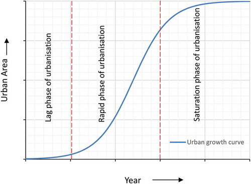
where $U_t$= urban area at time t, $U_{max}$= maximum developable urban land in the region, $U_0$= initial urban area, c = growth coefficient.

Spatial allocation module

The spatial allocation module in SUSM is a constrained stochastic urban cellular automaton, which is a stochastic artificial process for locating urban activities based on simple transition rules pertaining to local neighbourhoods. It is capable of simulating complex global patterns that mirror the spatial patterns of cities (Batty, 1997). It is composed of six fundamental elements: (i) the urban space or lattice, i.e. the geographic area of city, (ii) the state of a pixel in the urban space, i.e. either urban or non-urban state of pixel in SUSM, (iii) the neighbourhood used by the cellular automaton, (iv) the transition rules, (v) time step of the model, and (vi) stochastic component to simulate realistic patterns of urban growth. The neighbourhood around the cellular automaton (element (iii)) can be either von-Neumann (Batty, 1997), Moore (Clarke et al., 1997), circular (He et al., 2008) or a combination of the above. SUSM uses three types of neighbourhoods. These are Moore neighbourhoods, circular neighbourhoods with a five-pixel radius and circular neighbourhoods encompassing one square kilometre area around the pixel available for urbanization.

The transition rules are the engine of a cellular automaton (Torrens, 2000). The identification of transition rules is crucial to generate realistic urban growth patterns (Feng et al., 2016). The spatial allocation module applies transition rules to an urban area by utilizing three sub-modules: (i) developable land, (ii) seed planting and (ii) simulation sub-modules successively.

1. Developable land sub-module: Development control rules restrict urban development. Protected areas, biodiversity parks, reserved forest, water bodies and steep slope etc. are exempt from development. Thus, the developable land sub-model is used to select those non-urban pixels available for urban development.

2. Seed planting sub-module: The seed planting sub-module plants the urban seeds of urbanization. An urban seed is a starting point for urbanization. It uses two sub-modules to plant seeds. The first sub-module plants the seeds as per the location and year information provided by the town planner or by the SUSM user. By using this sub-module, the planners can plant the seeds of urbanization such as location of upcoming or proposed industrial firms, townships, or other proposed development projects to enable testing their impact upon urbanization and/or devise strategic planning measures. Cities are complex social and economic systems which show some degree of stochasticity (Barredo et al., 2003). A stochastic perturbation function (Equation (6)) is capable of producing a leap-frog or emergent development. Leap-frog or emergent development is a discontinuous development in the vicinity of an urbanized area, but it is not linked to the urban fringe or linear structures such as streets or railways (ribbon development). This development pattern may be due to institutional policy or social processes (Barredo et al., 2003; Feng et al., 2016). Thus, the second sub-module uses the stochastic perturbation function (Equation (6)), along with the transition potential derived from Equation (3) and two multi-criteria functions (namely, leap-frog (Equation (9)) and ribbon development (Equation (10)) to generate seeds at random locations. The second sub-module of the seed planting is designed to plant more seeds in the incentive/planned zones for urbanization.

   The stochastic perturbation function is defined as (White, Engelen, & Uljee, 1997):

   (6) $\vartheta =1+{\left[-\mathrm{l}\mathrm{n}\left(rand\right)\right]}^{\propto }$(6)

   where $\vartheta :$stochastic perturbation factor, $rand:$ a random value between 0 and 1, drawn from a uniform distribution and $\propto :$ a power parameter controls the size of the perturbation.

   These Two multi-criteria functions (namely, leap-frog and ribbon development) are used in SUSM to guide the planting of urban growth seeds in locations, which are far away from the existing development and major transportation networks. Both functions use the weighted sum of fuzzy layers pertaining to non-urban pixels produced by two fuzzy functions, namely FuzzyMSsmall (Equation (7)) and FuzzyMSlarge (Equation (8)). The FuzzyMSsmall and FuzzyMSlarge functions use mean and standard deviation of the input parameter/layer to scale the input values from “0” to “1”. The smaller input data values have a membership closer to 1 in FuzzyMSsmall, whereas larger input values have a membership closer to 1 in FuzzyMSlarge (Luo & Dimitrakopoulos, 2003).

   (7) $FuzzyMSsmall={\mu }_l\left(x\right)=\left\{\begin{array}{c}s/\left(x-m+s\right),x>m\\ 0,x\le m\end{array}\right.$(7)
   (8) $FuzzyMSlarge={\mu }_l\left(x\right)=\left\{\begin{array}{c}1-(s/\left(x-m+s\right)),x>m\\ 0,x\le m\end{array}\right.$(8)

   where$x=$ input data value; $m=$ mean value of input data layer, $s=$ standard deviation of input data values pertaining to non-urban pixel.

   (9) $Leap-frogcriteria\left(LFC\right)=\frac{{\mu }_s\left(DC{C}_{nu}\right)+{\mu }_s\left(DOG{V}_{nu}\right)+{\mu }_s\left(DR{D}_{nu}\right)+{\mu }_l\left(Per{U}_{nu}\right)}{4}$(9)
   (10) $Ribbondevelopmentcriteria\left(RDC\right)=\frac{{\mu }_s\left(DC{C}_{nu}\right)+{\mu }_s\left(DOG{V}_{nu}\right)+2\times {\mu }_s\left(DR{D}_{nu}\right)+{\mu }_l\left(Per{U}_{nu}\right)}{5}$(10)

   where ${\mu }_s()$ = FuzzyMSsmall function; ${\mu }_l()=$ Fuzzy-MSlarge function;$DC{C}_{nu}$ = Euclidian distance to city centre of non-urban pixels; $DOG{V}_{nu}=$ Euclidian distance to outgrowth village centres of non-urban pixels; $DR{D}_{nu}$ = Euclidian distance to major roads of non-urban pixels; $Per{U}_{nu}=$ Percentage of urban land around a non-urban pixel in one square kilometre area.

3. Urban growth simulation sub-module: The urban growth simulation module simulates urban growth around built-up pixels and urban seeds planted by the “seed planting sub-module”. It uses three transition rules, namely speculation, incentive and general growth rules. The speculation growth rule is used for simulation of non-urban pixels under land speculation. Land speculation can be represented by SUSM as the resistance of a non-urban pixel to be converted into urban although it has a high transition potential. In contrast, the incentive growth rule stimulates urban growth in the incentive zones. The general growth rule simulates the urban growth of non-urban pixels, which are neither under speculation nor located in incentive zones. For details about growth rules, please refer to supplement-1.

Validation module

Urban growth simulations can be used to test different development scenarios. Since urban growth models are an approximation of a complex adaptive urban system, validation of an urban growth model is essential to determine whether the model is capable of replicating the system behaviour in a given scenario with sufficient accuracy (Law, 2008; McDonnell, Azar, & White, 2013; Sargent, 2009). SUSM uses (i) a confusion matrix, (ii) an improved fuzzy kappa and (iii) a receiver operating characteristic (ROC) curve to evaluate the reliability of simulations under the observed historical trend scenario.

1. Confusion matrix: SUSM estimates a confusion matrix (Table 1) by comparing the simulated urban growth map with the observed urban growth map derived from remote sensing data to calculate the producer’s (Equation (11)), user’s (Equation (12)), and overall (Equation.(13)) accuracies along with the specificity (Equation (14)), “Matthews correlation coefficient (MCC)”(Equation (15)) and a “figure of merit” (Equation 16).

   (11) $Produce{r}^{\prime }saccuracy\left(Sensitivity\right)=\frac{Hits}{Hits+Misses}$(11)
   (12) $Use{r}^{\prime }saccuracy\left(Precision\right)=\frac{Hits}{Hits+Falsealarms}$(12)
   (13) $Overallaccuracy=\frac{Hits+Correctrejections}{Hits+Misses+Flasealarms+Correctrejections}$(13)
   (14) $Specificity\left(Truenegativerate\right)=\frac{Correctrejections}{Correctrejections+Falsealarms}$(14)
   (15) $Matthewscorrelationcoefficient\left(MCC\right)=\frac{\left(Hits\times Correctrejections\right)-\left(Falsealarms\times Misses\right)}{\sqrt{\left(Hits+Falsealarms\right)\left(Hits+Misses\right)\left(Correctrejections+Falsealarms\right)\left(Correctrejections+Misses\right)}}$(15)
   (16) $Figureofmerit=\frac{Hits}{Hits+Misses+Flasealarms}$(16)

   The producer’s accuracy of simulation refers to the “probability of detection”. It is a measure of the ability of the model to simulate urban pixels at the correct locations. The user’s accuracy refers to the precision of the model. The overall accuracy is a measure of agreement of the model results (simulated pixels both urban and non-urban at correct locations) with the observed reference derived from the remote sensing image. The user’s accuracy may not provide enough information if the class of interest (non-urban to urban) is small in comparison with the rest (Olofsson et al., 2014). In this case, we can use the specificity (true negative rate) as a measure of the model ability to avoid simulation of non-urban pixels that are not suitable for urbanization as an additional metric. The Matthews correlation coefficient (MCC) is regarded as a balanced measure to assess the quality of a binary classifier or a model when the classes are of very different sizes (Boughorbel, Jarray, & El-Anbari, 2017; Powers, 2011). The value of MCC varies between −1 and +1. A MCC value of +1 represents a perfect simulation, 0 is no better than random simulation and −1 indicates total disagreement between simulation and observation. The figure of merit is a ratio of the intersection of observed and simulated urban growth to the union of both (Pontius et al., 2008). A figure of merit value of 0 refers to no overlap between observed and simulated urban growth, whereas a value of “1” refers to a perfect match between simulated and observed urban growth.

2. Improved Fuzzy Kappa: The simulation of an urban pixel at the exact location is not possible in most cases due to the complex nature of urban growth processes (Wu et al., 2010). However, the spatial patterns simulated by the model should be similar to the observed patterns. Thus, the use of traditional kappa statistics, which uses a cell-by-cell comparison, is not suitable for assessing performance of simulation models. Hence, the improved fuzzy kappa (Hagen‐Zanker, 2009) is used to evaluate the SUSM results with respect to the observed urban growth derived from remote sensing data. The fuzzy kappa statistic (Hagen, 2003) uses fuzziness of location, based on the distance decay function, whereas improved fuzzy kappa accounts for the effect of spatial autocorrelation (for more details see Hagen-Zanker, 2009). The fuzzy kappa statistic achieves higher values (i.e. near to one) with the increase of matching categories found in the neighbourhood. The improved fuzzy kappa value can be calculated by using the following formula,

   (17) $K_{fuzzy}=\frac{P_o-P_e}{1-P_e}$(17)

   Table 1. Confusion matrix for validation of SUSM’s simulation.

   	Observed urban growth
   Simulated urban growth		Urban	Non-urban
   	Urban	Hits (H)	False alarms (F)
   	Non-urban	Misses (M)	Correct rejections (C)

   where $P_o=$ observed mean agreement and $P_e=$ expected agreement around a specified neighbourhood radius calculated by using an exponential distance decay function with a halving distance of two cells.

3. Receiver Operating Characteristic (ROC) curve: ROC is a two-dimensional graphical depiction of model performance (Fawcett, 2006). It is a useful measure to assess the performance of a model without a crisp classification about the state of the pixel (i.e. urban or non-urban). The ROC curve is used to assess the reliability of transition potential maps produced by SUSM. Thus, it enables validation of the model performance with respect to a specific location rather than committing to a specific quantity of change (Pontius & Schneider, 2001). An area under curve (AUC) value of 1 represents a perfect model, a AUC value greater than 0.5 represents a model, which is statistically better than random, and 0.5 represents agreement due to chance (Pontius & Schneider, 2001).

SUSM implementation

Test site

We tested the performance of SUSM for the Pune metropolis (Figure 3), which is the eighth largest urban agglomeration in India and is the southern headquarters of the Indian army. The test site contains two municipal corporations, i.e. Pune and Pimpri-Chinchwad, one municipality, i.e. Talegaon-Dabhade, three cantonment boards (areas under the military), i.e. Kirkee, Pune and Dehuroad and more than a 100 rural administrative bodies. It is bounded between latitudes 18° 19ʹ to 18°45ʹ N and longitudes 73°35ʹ to 74°12ʹ E with an area covering 1643 km².

Figure 3. Pune metropolis, PMC: Pune Municipal corporation, PCMC: Pimpiri Chinchwad Municipal Corporation, PCB: Pune Cantonment Board, KCB: Kirkee Cantonment Board.

The open economic policy by the Government of India in 1991 and the special economic zone policy by the state of Maharashtra in 2006 spurred widespread urbanization in the Pune metropolis attracting many global and national automobile, biotech and information technology firms. The population in Pune increased from 2.6 million in 1991 to 5.9 million in 2011 (Census of India, 2011). This rapid increase in population led to haphazard urban growth. In order to ensure sustainable urbanization, the state government constituted the Pune Metropolitan Regional Development Authority (PMRDA) in 2015. Thus, using Pune as a test site is not only a proof of concept of SUSM, but a successful model will also be rather useful in assisting the newly formed PMRDA in the planning process.

Input datasets

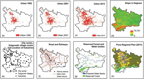
SUSM uses remote sensing derived land use and digital elevation maps as input and to validate simulation results. Moreover, GIS datasets such as roads, point locations of industries, transportation hubs, city and village centres and development plans, etc. can be derived from remote sensing data. In this study, we used a maximum-likelihood supervised classification of cloud free Landsat images from 4 December 1992, 3 November 2001 and 14 December 2013 to determine the urban extents for the respective years (Figure 4(a–c)). The producer’s accuracy of the extracted urban extents for 1992, 2001 and 2013 are 86.3%, 99.4% and 91.3%, respectively. The Aster DEM Version 2 was used to derive a slope in degrees (Figure 4(d)) map of the study area. The city centre and outgrowth village centres (Figure 4(e)), highway road network (Figure 4(f)), locations of major industries (Figure 4(e)) and railway stations (Figure 4(f)) were extracted from Google Earth, while reserved forests and water bodies (Figure 4(g)) were taken from the Survey of India and land use/land cover maps, respectively. The street network (Figure 4(f)) used in this study was extracted from the Open Street Map webserver. The boundaries of defence establishments and proposed land use of the study area were extracted from the development plan of Pune, Pimpri-Chinchwad municipal corporations and Maharashtra Regional and Town Planning office web portals.

Figure 4. Input datasets of SUSM.

Scenario development

Urban growth models may be used to analyse urban growth patterns for different scenarios. We prepared one simulation for model validation and two simulations to test scenarios, namely, with (i) urban planning information and ii) without urban plans. Urban growth of the Pune metropolis was simulated for the year 2013 based on the analysis of the urban growth process observed from 1992 to 2001.

1. The simulation for model validation was performed to evaluate the model performance. The model simulation was initialized with data from 2001 and the SUSM simulation runs until 2013. The locations of upcoming industrial areas were provided as “seeds” of urbanization and the observed urban growth was supplied as an “Intensity zone” of future urbanization in the validation scenario. Defence lands and recreational areas such as playgrounds and parks are restricted from urban development by assigning them with resistance coefficient value of 0.2. For open space in public and semi-public properties, a resistance coefficient of 0.3 is applied. Open lands under the Cantonment boards are assigned a resistance coefficient of 0.5, as these areas experienced minimal urban expansion during the period from 1992 to 2001(Kantakumar et al., 2016). In this validation run, the following locations of SEZ, major IT parks and townships are supplied as “seeds” of future urbanization (Table 2).

2. The official Pune metropolitan regional development plan of 2011 is used as input to SUSM in scenario 1: “Urban development plan”. The proposed residential, mixed land use, industrial and commercial lands are included as incentive zones of urbanization. Recreational spaces and green belts are restricted for development since they are assigned a resistance coefficient value of 0.2. Protected hill slopes, forests and afforestation lands are assigned a resistance coefficient value of 0.1, and agriculture land is assigned a resistance coefficient value of 0.8.

3. Scenario 2: “No urban development plan” is used to simulate urban expansion of Pune from 2001 to 2013 based only on the historic trend experienced from 1992 to 2001. Thus, urban planning measures are ignored in this simulation. Accordingly, urban seeds, incentive zones and zonal planning measure are not applied.

Table 2. Location of urban growth seeds supplied to SUSM in scenario 1.

Name of the seed, location	Year of seed planting	Latitude	Longitude
Hinjewadi SEZ Phase 1	2004	18°35ʹ13.22”N	73°44ʹ3.48”E
Magarpatta City, Hadapsar	2004	18°30ʹ44.59”N	73°55ʹ47.20”E
Hinjewadi SEZ Phase 2	2008	18°35ʹ41.24”N	73°42ʹ28.48”E
Eon IT park, Kharadi	2008	18°33ʹ0.32”N	73°57ʹ8.27”E
Hinjewadi SEZ Phase 3	2011	18°34ʹ45.23”N	73°40ʹ52.52”E

Transition potential estimation

Seven spatial variables, namely, slope, distance to city centre (DCcn), major roads (DRd), distance to railways stations (DRly), industries (DInd), built-up areas (DBul) and percentage of urban pixels in one square kilometre circular neighbourhood (%Urb), pertaining to the period of 1992–2001 are used in Equation (4) and Equation (3) to estimate the regression coefficients of the logistic regression (Table 3) and the transition potential of non-urban pixels.

Table 3. Logistic regression coefficients for the period of 1992 to 2001.

	1991–2001
Spatial variable	β		S.E.
Intercept	3.215	***	0.338
Slope	−0.015		0.030
Distance to city centre	−0.051	***	0.015
Distance to important roads	−0.133	*	0.069
Distance to railway stations	−0.123	***	0.026
Distance to major industries	−0.032	***	0.012
Distance to built-up	−2.531	***	0.252
Percentage of urban in one sq.km	0.020	**	0.008
Nagelkerke’s R^2	0.64
AIC	944.59
Moran’s I of Residuals	0.0699***

***p < .01; **p < .05; *p < 0.1

Projecting urban land demand

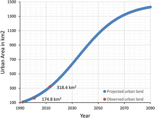
The Pune metropolis witnessed a massive increase in urban area of about 215.4 km² from 107.5 km² in 1992 to 162.4 km² in 2001 and to 322.9 km² in 2013 with an annual expansion rate of 6.1 km² per annum from 1992 to 2001 and 13.4 km² per annum from 2001 to 2013. The maximum developable urban land ($U_{max}$ = 1481 km²) is estimated by subtracting the areas covered by reserved forest (132 km²) and water bodies (30 km²) from the total area of the study region (1643 km²). The historic urban growth trend, i.e. the annual expansion rate of 6.1 km² per annum for the period of 1992–2001 is used to estimate the growth coefficient (c = 0.0596) of Pune metropolis. Figure 5 shows the projection of the urban land up to 2090 using the urban land demand module (see section 2.3.1). Table 4 shows the comparison of projected urban land to the remote sensing derived urban growth.

Table 4. Comparison of projected urban area to the remote sensing–derived urban area.

Year	Observed urban area (km^2) from remote sensing data	Projected urban area (km^2) using SUSM	Discrepancy
1990	107.5	–
2001	162.4	174.8	12.4
2013	322.9	318.4	−4.5

Figure 5. The urban growth curve of Pune metropolis (total area:1643 km²).

SUSM simulations of Pune

Validation

The transition potential derived from the transition potential sub-model for the period of 1992 to 2001 and the urban land demand projected from the allocation module (Figure 5) were used in the simulation of the validation run to simulate the urban expansion of Pune for the year 2013. Figure 6 shows a map of the estimated urban growth transition potential and the simulation result for 2013.

Figure 6. SUSM simulations used for validation (a) Urban growth transition potential and (b) Urban growth simulation maps of 2013.

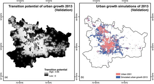
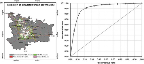
The simulated urban growth for 2013 is compared with the observed urban growth derived from a LANDSAT image of the same year. Table 5 shows the scores of the fit metrics used to validate the SUSM simulations. Figure 7(a) shows a pixel-by-pixel comparison of SUSM’s urban growth simulation and the LANDSAT classification result. Figure 7(b) shows the ROC curve estimated by comparing the modelled urban growth transition potentials with the respective observed urban growth from 2001 to 2013. The area under ROC curve with a value 0.90 shows that SUSM accurately estimates the transition potential of a non-urban pixel to be urbanised.

Table 5. Validation results of SUSM.

Fit metric	Score	95% C.I.
Producer’s accuracy (Sensitivity)	75.76%	[75.38%, 76.14%]
User’s accuracy (Precision)	78.85%	[78.66%, 79.04%]
Overall accuracy	95.06%	[95.02%, 95.09%]
Specificity (True negative rate)	97.46%	[97.44%, 97.49%]
Matthews correlation coefficient	0.75	–
Figure of fit	0.63	–
Fuzzy Kappa	0.81	–
AUC	0.90	–

Figure 7. (a) Validation map showing the pixel level comparison of SUSM’s urban growth simulation with respect to observed urban growth from 2001 to 2013. (b) ROC curves of modelled urban growth transition potential of Pune for 2013.

Simulation results using urban development plans and without urban development plans

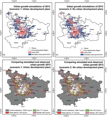
SUSM is used to simulate the urban growth of Pune from 2001 to 2013 to assess the impact of urban development plans on Pune’s urbanization by comparing two scenarios: 1: using urban development plans as input and 2: without urban development plans. A strict implementation of the development plan (scenario 1) might result in an urban growth of Pune for the year 2013 as shown in Figure 8(a). Figure 8(b) shows the modelled urban growth of Pune for the year 2013 for scenario 2: no urban development plan. Figure 8(c,d) show the comparison of simulated urban growth with observed urban growth for these two scenarios. From Figure 8, we can see that the simulation based on scenario 2 performed marginally better (hits: 85.5 km²) than the simulation based on the urban development plan, i.e. scenario 1 (hits: 77.7 km²). The urban growth patterns simulated under the “no urban development plan scenario” (scenario 2) are consistent with the urban growth pattern observed for 2013.

Figure 8. (a) Urban growth simulations based on scenario 1: urban development plan (i.e. PMR regional development plan), (b) Urban growth simulations based on scenario 2: no urban development plan (i.e. business as usual based on the historic trend observed from 1992–2001 and without any future development measures), (c) and (d) comparison of simulated growth of Pune based on scenario 1 and scenario 2, respectively, with observed urban growth from 2001 to 2013.

Discussion

The results of SUSM simulations are discussed with respect to (i) the performance of SUSM and (ii) urban planning processes.

Performance of SUSM

The assessment of performance of an urban growth model by comparison to a measured reference is essential to understand the potentials and limits of the model. The results of the validation run show that SUSM simulates urban growth with a producer’s accuracy of 75.76% and a user’s accuracy of 78.85%. SUSM yields producer’s accuracies ranging from 75.38% to 76.14% and user’s accuracies ranging from 78.66% to 79.04% at 95% confidence level (Table 5). The transition potentials maps of SUSM provide a 90% agreement. The overall accuracy of spatial simulations of SUSM is 95.06%. However, this cannot be interpreted as a direct measure of the SUSM simulation accuracy due to the fact that the persistence of non-urban pixels is far higher than the urban growth observed in the test site. Thus, SUSM uses a balanced measure namely the “Matthews correlation coefficient (MCC)” to assess the quality of model simulations (Boughorbel et al., 2017; Powers, 2011). The MCC value of 0.75 reveals that SUSM captures urban growth dynamics of Pune very well.

Using the reported score of fit, user’s and producer’s accuracies (see table-1 in supplement) show that the SUSM performance is slightly better as compared to other urban growth and land use models. Eleven different models were used for this comparison: i.e. CLUE, CLUES-S, Geomod, Environment Explorer, Land Use Scanner, Logistic regression, LTM, SAMADA, SLEUTH (Pontius et al., 2008), Patch-logistic-CA and cell/pixel based logistic-CA (Chen, 2016; Li, Gong, Yu, & Hu, 2017) and SLEUTH(Yin, Kong, Yang, James, & Dronova, 2018). Also, the fuzzy kappa value of SUSM simulation is slightly higher than the reported values in other studies (Long, Han, Lai, & Mao, 2013; Vliet et al., 2009; Wu et al., 2010) (refer to table-2 in supplement). Simulations based on urban growth models are affected by many parameters such as quality of the input datasets, scenarios, initial conditions, modelling concepts and techniques used (Batty & Torrens, 2005). However, due to differences in the model setup, inputs, locations etc., the comparison discussed need to be assessed with caution.

Urban planning and SUSM

Simulation models are often used to inform rather than predict. Thus, the practical utility of an urban growth simulation model hinges on its applicability to assess the impact of planning measures or to devise strategic plans to avoid undesirable effects. Here, we incorporated the official regional development plan of 2011 of Pune via scenario 1 into SUSM. The simulation revealed that the strict implementation of the regional development plan might have resulted in spatial patterns of urbanization as shown in Figure 8(a). These patterns of spatial simulation resemble the proposed growth patterns in the multiple nuclei model proposed by Harris and Ullman (1945). The simulation based on scenario 1 encompasses 48% of the urban growth experienced by Pune from 2001 to 2013. The important result from the simulations from scenario 1 are: (i) Pune’s Regional development plan of 2011 allotted more land for residential land use in the Talegaon municipality and Urli-Kanchan villages, even though they have less potential for future urbanization (refer Figures 4(h), 8(a,c)). (ii) The simulation of ribbon development along the Saswad road and the Pune-Hinjewadi road reveals the importance of these roads, which were not adequately considered during the planning process. (iii) Most of the simulated growth agreed with the observed growth in PMC and PCMC. This reveals that the development plan was more successful in the municipal corporation limits as compared to the notified town and outgrowth villages, suggesting the need for an overarching nodal authority to implement the planning measures to avoid haphazard and unsustainable growth of Pune. In 2015, the Maharashtra state government formed Pune Metropolitan Regional Development Authority (PMRDA) as a nodal planning agency for Pune metropolis.

The SEZ namely Hinjawadi phase II and phase III were not proposed/planned in the Pune’s regional development of 2011. However, plans from Hinjawadi phase II and phase III SEZs near the foot hills of the Western Ghats of India spurred urbanization along the valleys. This unforeseen and unplanned urbanization has not only led to heavy traffic congestion but also poses a threat to the flora and fauna in foothills of the Western Ghats. The impact of such development as well as the influence of SEZs on urban growth can be assessed by utilizing the seed planting sub-module of SUSM.

The spatial patterns simulated without using the urban development plan (scenario 2) are more consistent with the observed urbanization patterns from 2001 to 2013 in comparison with the results using the urban development plan (scenario 1) (Figures 4(c) and 8). Scenario 2 effectively captures the ribbon development along highways. In-spite of the fact that no “seeds” are supplied in scenario 2, the simulation of urban growth around Hinjawadi, Wakad, Pashan, Kharadi villages and ribbon development along the Pune-Saswad road reveals the importance of these areas in future urbanization. Thus, planning of sufficient road infrastructure in these areas could have avoided the heavy traffic congestion presently faced by citizens of Pune. The business as usual simulation suggests a lower urbanization rate around Talegaon, Dehu and Urli-Kanchan areas. This may be due to land speculations. However, the regional development plan proposed larger residential areas, which might be due to proposed industries in these areas. Such mismatches of land use allocations are often a result of imposing a top-down planning process for the sake of rational planning and may nevertheless result in irrational outcomes of urbanization (Mahadevia & Joshi, 2009). The simulation result without urban planning scenario is marginally better (53% of match with observed growth) than the result achieved when using the urban development plan as input (48% match). The inclusion of urban seeds with strategic importance might further improve the accuracy of SUSM simulations when using scenario 2 (no development plan). Thus, SUSM simulations can help planners to test urban or regional development plans by analysing the impacts of proposed planning measures through scenario analysis.

Conclusion

The practical utility of urban growth simulation models hinges on their ability to assess the implication of development plans and policies on future urbanization of a city. This paper described the SUSM using generally available remote sensing datasets as input and it exemplified the use of SUSM in assessing the regional development plan of the rapidly growing Pune metropolis in India. The results show that (i) SUSM is capable of simulating the urban expansion with a user accuracy of 79%. (ii) The development plans provide an envelope for urban development, but do not provide a prediction of urban growth. (iii) The urban growth patterns simulated based on no urban planning measures (scenario 2) are consistent with the urban growth patterns derived from remote sensing data and marginally more accurate than the simulations based on urban planning measures (scenario 1). This study showed that SUSM can be used effectively to assess the impact of development plans upon a rapidly growing metropolis such as Pune. The use of widely available, inexpensive remote sensing datasets, logistic regression and a constrained stochastic cellular automaton with fairly simple transition rules offers transferability and applicability of SUSM to other cities.

In this research, we used simple scenarios to assess urban growth, i.e. regional development plan and business as usual scenario. Additional research is needed to explore the full potential of the scenario development module of SUSM by developing and testing more dynamic and complex scenarios, which includes socioeconomic datasets to understand the implication of urban plans and polices. The integration of other machine learning algorithms such as artificial neural networks and random forest besides the logistic regression model into SUSM calibration method is another future direction for development.

Acknowledgments

We greatly acknowledge Landsat data from EROS data centre, USGS, Sioux Falls, ASTER DEM data from Japan space system and Census data from Census of India. The authors gratefully appreciate the support of the director and other staff members of Maharashtra and Goa Geospatial Data Centre, Pune. Special thanks go to Karen Schneider for proof reading the manuscript.

Disclosure statement

No potential conflict of interest was reported by the authors.

Supplementary material

Supplemental data for this article can be accessed here

References

- Aguayo, M.I., Wiegand, T., Azócar, G.D., Wiegand, K., & Vega, C.E. (2007). Revealing the driving forces of mid-cities urban growth patterns using spatial modeling: A case study of Los Ángeles, Chile. Ecology and Society, 12, 1. Retrieved from http://www.ecologyandsociety.org/vol12/iss1/art13/
- Alsharif, A.A.A., & Pradhan, B. (2013). Urban Sprawl analysis of Tripoli Metropolitan City (Libya) using remote sensing data and multivariate logistic regression model. Journal of the Indian Society of Remote Sensing, 42(1), 149–163. doi:10.1007/s12524-013-0299-7
- Arsanjani, J., Helbich, M., Kainz, W., & Darvishi Boloorani, A. (2013). Integration of logistic regression, Markov chain and cellular automata models to simulate urban expansion. International Journal of Applied Earth Observation and Geoinformation, 21, 265–275. doi:10.1016/j.jag.2011.12.014
- Barredo, J.I., Kasanko, M., McCormick, N., & Lavalle, C. (2003). Modelling dynamic spatial processes: Simulation of urban future scenarios through cellular automata. Landscape and Urban Planning, 64(3), 145–160. doi:10.1016/S0169-2046(02)00218-9
- Batty, M. (1997). Cellular automata and urban form: A primer. Journal of the American Planning Association, 63(2), 266–274. doi:10.1080/01944369708975918
- Batty, M. (2008). Fifty years of urban modeling: Macro-statics to micro-dynamics. In P.D.D.h c S. Albeverio, D. Andrey, P. Giordano, & D.A. Vancheri (Eds.), The dynamics of complex urban systems (pp. 1–20). Physica-Verlag HD. Retrieved from (), (pp.). .http://link.springer.com/chapter/10.1007/978-3-7908-1937-3_1
- Batty, M. (2012). Building a science of cities. Cities, 29(Supplement 1), S9–S16. doi:10.1016/j.cities.2011.11.008
- Batty, M., & Torrens, P.M. (2005). Modelling and prediction in a complex world. Futures, 37(7), 745–766. doi:10.1016/j.futures.2004.11.003
- Batty, M., Longley, P., & Fotheringham, S. (1989). Urban growth and form: Scaling, fractal geometry, and diffusion-limited aggregation. Environment and Planning A, 21(11), 1447–1472. doi:10.1068/a211447
- Berry, B.J.L. (2008). Urbanization. In J.M. Marzluff, E. Shulenberger, W. Endlicher, M. Alberti, G. Bradley, C. Ryan, & C. ZumBrunnen (Eds.), Urban ecology (pp. 25–48). Springer US. Retrieved from http://link.springer.com/chapter/10.1007/978-0-387-73412-5_3
- Bhatta, B. (2010). Analysis of urban growth and sprawl from remote sensing data. Heidelberg, Germany: Springer Science & Business Media.
- Borges, R.C., Dos Santos, F.V., Caldas, V.G., & Lapa, C.M.F. (2015). Use of geographic information system (GIS) in the characterization of the Cunha Canal, Rio de Janeiro, Brazil: Effects of the urbanization on water quality. Environmental Earth Sciences, 73(3), 1345–1356. doi:10.1007/s12665-014-3493-1
- Boughorbel, S., Jarray, F., & El-Anbari, M. (2017). Optimal classifier for imbalanced data using Matthews correlation coefficient metric. PLOS ONE, 12(6), e0177678. doi:10.1371/journal.pone.0177678
- Butsch, C., Kumar, S., Wagner, P.D., Kroll, M., Kantakumar, L.N., Bharucha, E., … Kraas, F. (2017). Growing ‘smart’? Urbanization processes in the Pune urban agglomeration. Sustainability, 9(12), 2335. doi:10.3390/su9122335
- Census of India. (2011). Provisional population totals. New Delhi: Office of the Register General and Census Commissioner.
- Chen, Y. (2016). Defining urban and rural regions by multifractal spectrums of urbanization. Fractals, 24(01), 1650004. doi:10.1142/S0218348X16500043
- Cheng, J., & Masser, I. (2003). Urban growth pattern modeling: A case study of Wuhan city, PR China. Landscape and Urban Planning, 62(4), 199–217. doi:10.1016/S0169-2046(02)00150-0
- Clarke, K.C., Hoppen, S., & Gaydos, L. (1997). A self-modifying cellular automaton model of historical urbanization in the San Francisco Bay Area. Environment and Planning B: Planning and Design, 24(2), 247–261. doi:10.1068/b240247
- Crooks, A.T. (2006). Exploring cities using agent-based models and GIS (Working Paper-109). London, UK: CASA, University College London.
- Dieleman, F., & Wegener, M. (2004). Compact city and urban sprawl. Built Environment, 30(4), 308–323. doi:10.2148/benv.30.4.308.57151
- Ellefsen, R., Swain, P., & Wray, J. (1973). Urban land-use mapping by machine processing of ERTS-1 multi spectral data: A San Francisco Bay Area example. LARS Technical Reports, 115, 2A–10.
- Fawcett, T. (2006). An introduction to ROC analysis. Pattern Recognition Letters, 27(8), 861–874. doi:10.1016/j.patrec.2005.10.010
- Feng, Y., Liu, Y., & Batty, M. (2016). Modeling urban growth with GIS based cellular automata and least squares SVM rules: A case study in Qingpu–Songjiang area of Shanghai, China. Stochastic Environmental Research and Risk Assessment, 30(5), 1387–1400. doi:10.1007/s00477-015-1128-z
- Grimm, N.B., Grove, J.M., Pickett, S.T.A., & Redman, C.L. (2008). Integrated approaches to long-term studies of urban ecological systems. In J.M. Marzluff, E. Shulenberger, W. Endlicher, M. Alberti, G. Bradley, C. Ryan, & C. ZumBrunnen (Eds.), Urban ecology (pp. 123–141). Springer US. Retrieved from http://link.springer.com/chapter/10.1007/978-0-387-73412-5_8
- Hagen, A. (2003). Fuzzy set approach to assessing similarity of categorical maps. International Journal of Geographical Information Science, 17(3), 235–249. doi:10.1080/13658810210157822
- Hagen‐Zanker, A. (2009). An improved Fuzzy Kappa statistic that accounts for spatial autocorrelation. International Journal of Geographical Information Science, 23(1), 61–73. doi:10.1080/13658810802570317
- Han, J., Hayashi, Y., Cao, X., & Imura, H. (2009). Application of an integrated system dynamics and cellular automata model for urban growth assessment: A case study of Shanghai, China. Landscape and Urban Planning, 91(3), 133–141. doi:10.1016/j.landurbplan.2008.12.002
- Harris, C.D., & Ullman, E.L. (1945). The nature of cities. The Annals of the American Academy of Political and Social Science, 242, 7–17. doi:10.1177/000271624524200103
- He, C., Okada, N., Zhang, Q., Shi, P., & Li, J. (2008). Modelling dynamic urban expansion processes incorporating a potential model with cellular automata. Landscape and Urban Planning, 86(1), 79–91. doi:10.1016/j.landurbplan.2007.12.010
- Hosmer, D.W., & Lemeshow, S. (2004). Applied logistic regression. New York, NY: John Wiley & Sons.
- Imhoff, M.L., Lawrence, W.T., Stutzer, D.C., & Elvidge, C.D. (1997). A technique for using composite DMSP/OLS “city lights” satellite data to map urban area. Remote Sensing of Environment, 61(3), 361–370. doi:10.1016/S0034-4257(97)00046-1
- Itami, R.M. (1994). Simulating spatial dynamics: Cellular automata theory. Landscape and Urban Planning, 30(1–2), 27–47. doi:10.1016/0169-2046(94)90065-5
- Jensen, J.R. (1981). Urban change detection mapping using landsat digital data. The American Cartographer, 8(2), 127–147. doi:10.1559/152304081784447318
- Kantakumar, L.N., Kumar, S., & Schneider, K. (2016). Spatiotemporal urban expansion in Pune metropolis, India using remote sensing. Habitat International, 51, 11–22. doi:10.1016/j.habitatint.2015.10.007
- Kavilkar, R.D. (2018). Influence of socialism and neo-liberalism and their policies on growth of Indian cities. Springer International Publishing. doi:10.1007/978-3-319-76267-8_8
- Kong, F., Yin, H., Nakagoshi, N., & James, P. (2012). Simulating urban growth processes incorporating a potential model with spatial metrics. Ecological Indicators, 20(Supplement C), 82–91. doi:10.1016/j.ecolind.2012.02.003
- Law, A.M. (2008). How to build valid and credible simulation models. In Proceedings of the 40th Conference on Winter Simulation (pp. 39–47). Miami, FL: Winter Simulation Conference.
- Li, X., Zhou, W., & Ouyang, Z. (2013). Forty years of urban expansion in Beijing: What is the relative importance of physical, socioeconomic, and neighborhood factors?. Applied Geography, 38, 1–10. doi:10.1016/j.apgeog.2012.11.004
- Li, X., Gong, P., Yu, L., & Hu, T. (2017). A segment derived patch-based logistic cellular automata for urban growth modeling with heuristic rules. Computers, Environment and Urban Systems, 65(SupplementC), 140–149. doi:10.1016/j.compenvurbsys.2017.06.001
- Liu, Y., & Feng, Y. (2012). A logistic based cellular automata model for continuous urban growth simulation: A case study of the Gold Coast City, Australia. In Agent-based models of geographical systems (pp. 643–662). Dordrecht: Springer. doi:10.1007/978-90-481-8927-4_32
- Long, Y., Han, H., Lai, S.-K., & Mao, Q. (2013). Urban growth boundaries of the Beijing Metropolitan Area: Comparison of simulation and artwork. Cities, 31, 337–348. doi:10.1016/j.cities.2012.10.013
- López, E., Bocco, G., Mendoza, M., & Duhau, E. (2001). Predicting land-cover and land-use change in the urban fringe: A case in Morelia City, Mexico. Landscape and Urban Planning, 55(4), 271–285. doi:10.1016/S0169-2046(01)00160-8
- Luo, X., & Dimitrakopoulos, R. (2003). Data-driven fuzzy analysis in quantitative mineral resource assessment. Computers & Geosciences, 29(1), 3–13. doi:10.1016/S0098-3004(02)00078-X
- Mage, D., Ozolins, G., Peterson, P., Webster, A., Orthofer, R., Vandeweerd, V., & Gwynne, M. (1996). Urban air pollution in megacities of the world. Atmospheric Environment, 30(5), 681–686. doi:10.1016/1352-2310(95)00219-7
- Mahadevia, D., & Joshi, R. (2009). Subversive urban development in India: Implications on planning education. 10th Congress of the Association of Planning Schools of Asia (APSA) (pp. 1–18), Ahmedabad, IN: Congress of the Association of Planning Schools of Asia, CEPT University, Ahmedabad.
- McDonnell, G., Azar, A.T., & White, J.C. (2013). Renal system dynamics modeling. In Modeling and control of dialysis systems (pp. 1275–1320). Berlin, Heidelberg: Springer. doi:10.1007/978-3-642-27558-6_11
- Ministry of urban development. (2015). Smart cities - mission statement and guidelines. Ministry of Urban Development, Govt. Of India. Retrieved from http://moud.gov.in/
- Moghadam, H.S., & Helbich, M. (2013). Spatiotemporal urbanization processes in the megacity of Mumbai, India: A Markov chains-cellular automata urban growth model. Applied Geography, 40, 140–149. doi:10.1016/j.apgeog.2013.01.009
- Olofsson, P., Foody, G.M., Herold, M., Stehman, S.V., Woodcock, C.E., & Wulder, M.A. (2014). Good practices for estimating area and assessing accuracy of land change. Remote Sensing of Environment, 148, 42–57. doi:10.1016/j.rse.2014.02.015
- Osman, T., Divigalpitiya, P., & Arima, T. (2016). Driving factors of urban sprawl in Giza governorate of the Greater Cairo Metropolitan Region using a logistic regression model. International Journal of Urban Sciences, 20(2), 206–225. doi:10.1080/12265934.2016.1162728
- Pontius, R.G., Boersma, W., Castella, J.-C., Clarke, K., de Nijs, T., Dietzel, C., … Verburg, P.H. (2008). Comparing the input, output, and validation maps for several models of land change. The Annals of Regional Science, 42(1), 11–37. doi:10.1007/s00168-007-0138-2
- Pontius, R.G., Jr., & Schneider, L.C. (2001). Land-cover change model validation by an ROC method for the Ipswich watershed, Massachusetts, USA. Agriculture, Ecosystems & Environment, 85(1–3), 239–248. doi:10.1016/S0167-8809(01)00187-6
- Powers, D.M. (2011). Evaluation: from precision, recall and F-measure to ROC, informedness, markedness and correlation.
- Ramachandra, T.V., Aithal, B.H., & Sowmyashree, M.V. (2014). Urban structure in Kolkata: Metrics and modelling through geo-informatics. Applied Geomatics, 6(4), 229–244. doi:10.1007/s12518-014-0135-y
- Roy, A. (2009). Why India cannot plan its cities: Informality, insurgence and the idiom of urbanization. Planning Theory, 8(1), 76–87. doi:10.1177/1473095208099299
- Sandamali, S.P.I., Kantakumar, L.N., & Sivanantharajah, S. (2018). Remote sensing data and SLEUTH urban growth model: As decision support tools for urban planning, remote sensing data and SLEUTH urban growth model: As decision support tools for urban planning. Chinese Geographical Science, 28(2), 274–286. doi:10.1007/s11769-018-0946-6
- Santé, I., García, A.M., Miranda, D., & Crecente, R. (2010). Cellular automata models for the simulation of real-world urban processes: A review and analysis. Landscape and Urban Planning, 96(2), 108–122. doi:10.1016/j.landurbplan.2010.03.001
- Sargent, R.G. (2009). Verification and validation of simulation models. In Simulation Conference (WSC), Proceedings of the 2009 Winter (pp. 162–176). Austin, TX: IEEE.
- Senge, P.M., & Forrester, J.W. (1980). Tests for building confidence in system dynamics models. System Dynamics, TIMS Studies in Management Sciences, 14, 209–228.
- Seto, K.C., Fragkias, M., Güneralp, B., & Reilly, M.K. (2011). A meta-analysis of global urban land expansion. PLoS ONE, 6(8), e23777. doi:10.1371/journal.pone.0023777
- Shafizadeh-Moghadam, H., Asghari, A., Tayyebi, A., & Taleai, M. (2017). Coupling machine learning, tree-based and statistical models with cellular automata to simulate urban growth. Computers, Environment and Urban Systems, 64, 297–308. doi:10.1016/j.compenvurbsys.2017.04.002
- Shrestha, M.K., York, A.M., Boone, C.G., & Zhang, S. (2012). Land fragmentation due to rapid urbanization in the Phoenix Metropolitan Area: Analyzing the spatiotemporal patterns and drivers. Applied Geography, 32(2), 522–531. doi:10.1016/j.apgeog.2011.04.004
- Tayyebi, A., Pijanowski, B.C., & Tayyebi, A.H. (2011). An urban growth boundary model using neural networks, GIS and radial parameterization: An application to Tehran, Iran. Landscape and Urban Planning, 100(1), 35–44. doi:10.1016/j.landurbplan.2010.10.007
- Torrens, P.M. (2000). How cellular models of urban systems work (1. Theory). Retrieved from http://eprints.ucl.ac.uk/1371/1/paper28.pdf
- United Nations. (2012). World urbanization prospects: The 2011 revision (pp. 1–50). New York: Department of Economic and Social Affairs (DESA).
- United Nations. (2016). The world’s cities in 2016 – data booklet. Department of Economic and Social Affairs, Population Division. Retrieved from http://www.un.org/en/development/desa/population/publications/pdf/urbanization/the_worlds_cities_in_2016_data_booklet.pdf
- van Vliet, J., White, R., & Dragicevic, S. (2009). Modeling urban growth using a variable grid cellular automaton. Computers, Environment and Urban Systems, 33(1), 35–43. doi:10.1016/j.compenvurbsys.2008.06.006
- Verburg, P.H., van Eck, J.R.R., de Nijs, T.C.M., Dijst, M.J., & Schot, P. (2004). Determinants of land-use change patterns in the Netherlands. Environment and Planning B: Planning and Design, 31(1), 125–150. doi:10.1068/b307
- Wagner, P.D., Bhallamudi, S.M., Narasimhan, B., Kantakumar, L.N., Sudheer, K.P., Kumar, S., … Fiener, P. (2016). Dynamic integration of land use changes in a hydrologic assessment of a rapidly developing Indian catchment. Science of the Total Environment, 539, 153–164. doi:10.1016/j.scitotenv.2015.08.148
- White, R., Engelen, G., & Uljee, I. (1997). The use of constrained cellular automata for high-resolution modelling of urban land-use dynamics. Environment and Planning B: Planning and Design, 24(3), 323–343. doi:10.1068/b240323
- Wu, D., Liu, J., Wang, S., & Wang, R. (2010). Simulating urban expansion by coupling a stochastic cellular automata model and socioeconomic indicators. Stochastic Environmental Research and Risk Assessment, 24(2), 235–245. doi:10.1007/s00477-009-0313-3
- Yin, H., Kong, F., Yang, X., James, P., & Dronova, I. (2018). Exploring zoning scenario impacts upon urban growth simulations using a dynamic spatial model. Cities. doi:10.1016/j.cities.2018.04.010
- Zha, Y., Gao, J., & Ni, S. (2003). Use of normalized difference built-up index in automatically mapping urban areas from TM imagery. International Journal of Remote Sensing, 24(3), 583–594. doi:10.1080/01431160304987