Fusion of Sentinel-1 data with Sentinel-2 products to overcome non-favourable atmospheric conditions for the delineation of inundation maps

2

ABSTRACT

729Sentinel-1 data are an alternative for monitoring flooded inland surfaces during cloudy periods. Supervised classification approaches with a single-trained model for the entire image demonstrate poor accuracy due to confusing backscatter conditions of the inundated areas in relation with the prevailing land cover features. This study follows instead a pixel-centric approach, which exploits the varying backscatter values of each pixel through a time series of Sentinel-1 images to train local Random Forest classification models per 3×3 pixels, and classifies each pixel in the target Sentinel-1 image, accordingly. Reference training data is retrieved from the timely close Sentinel-2-derived inundation maps. This study aims to identify the furthest mean day difference between the target Sentinel-1 image and available Sentinel-2 high accurate inundation maps (kappa coefficient—k > 0.9) that allows for the estimation of credible inundation maps for the Sentinel-1 target date. Various combinations of Sentinel-2 and Sentinel-1 training datasets are examined. The evaluation for eight target dates confirms that a Sentinel-1 inundation map with a k of 0.75 on average can be generated, when mean day difference is less than 30 days. The increment of the considered Sentinel-2 maps allows for the estimation of Sentinel-1 inundation maps with higher accuracy.

KEYWORDS:

• Inundation mapping
• Sentinel-1
• Sentinel-2
• wetland
• marshland
• pixel-centric supervised classification

Introduction

Wetlands partially exhibit areas with shallow water levels covered by emergent plants during the growing and water saturation period (e.g. seasonal marshlands) (Guo, Li, Sheng, Xu, & Wu, 2017). These are important for water-related ecosystem services including water filtration, shoreline protection and food provision. Additionally, they are key habitats for wildlife including native and migratory water-bird species (Green, Bustamante, Janss, Fernández-Zamudio, & Díaz-Paniagua, 2016; Guo et al., 2017; Wang & Yésou, 2018). Wetlands are also popular destinations for recreational activities including hiking, fishing, bird watching and photography (Musamba, Boon, Ngaga, Giliba, & Dumulinyi, 2012; Park, Lee, & Peters, 2017). They constitute significant nature’s reserves for biodiversity preservation (Beatty, Kesler, Webb, Raedeke, Naylor, & Humburg, 2014; Zhang, Wang, Hu, & Ho, 2010).

The combined effect of climate change and human activities poses a threat to wetlands’ functions and services. In particular, more frequent droughts (especially in the Mediterranean coasts) and wetlands reclamation for agriculture purposes could cause shrinkage of wetland area extent, disturbance of the available to-be-flooded zone, decrease of the annual biomass production, and habitat degradation. Therefore, monitoring of the spatiotemporal variability of the hydrological cycle of a wetland is important for taking timely appropriate mitigation actions. Satellite data, which are available at no or low cost, offer the possibility to monitor the extent of water coverage over wetlands frequently and with high accuracy. Satellite-based inundation maps can be also used in hydrological models for the generation of flood mapping forecasts (Giustarini, Chini, Hostache, Pappenberger, & Matgen, 2015; Khan et al., 2011; Ramos-Fuertes, Marti-Cardona, Bladé, & Dolz, 2014).

Multi-spectral satellite data are preferred for the estimation of water coverage under cloud-free weather conditions due to their high spectral correlation with the open water surface on the ground and respective mapping accuracy (Irwin, Beaulne, Braun, & Fotopoulos, 2017). Several methods apply thresholds to one or more spectral bands or indices including short-wave infrared bands (Díaz-Delgado, Aragonés, Afán, & Bustamante, 2016; Kordelas, Manakos, Aragonés, Díaz-Delgado, & Bustamante, 2018) and indices such as Normalised Difference Water Index (NDWI) (Du et al., 2016; Sun, Sun, Chen, & Gong, 2012; Yang & Lu, 2013) and the Modified NDWI (Donchyts, Schellekens, Winsemius, Eisemann, & van de Giesen, 2016; Du et al., 2016; Sun et al., 2012), whose estimation relies on green and near-infrared or short-wave infrared (SWIR) bands. Other approaches perform classification relying on machine learning algorithms, such as Random Forests (RFs) (Feng, Gong, Liu, & Li, 2015; Ko, Kim, & Nam, 2015), and support vector machines (Nandi, Srivastava, & Shah, 2017; Sarp & Ozcelik, 2017).

However, as flood events take place during periods of extended cloud coverage the exploitation of multi-spectral data may become questionable. Thus, space-borne radar data may be the only wide covering real time resource for generating frequently updated inundation maps. Images from Radarsat-2 (Behnamian et al., 2017; Bolanos, Stiff, Brisco, & Pietroniro, 2016; Li & Wang, 2015; Nakmuenwai, Yamazaki, & Liu, 2017), TerraSAR-X (Gstaiger, Huth, Gebhardt, Wehrmann, & Kuenzer, 2012; Hahmann & Wessel, 2010; Martinis, Twele, & Voigt, 2009), Envisat ASAR (Gstaiger et al., 2012; Henry, Chastanet, Fellah, & Desnos, 2006; Marti-Cardona, Dolz-Ripolles, & Lopez-Martinez, 2013), COSMO-SkyMed (Pierdicca, Pulvirenti, Chini, Guerriero, & Candela, 2013) and ALOS PALSAR (Arnesen et al., 2013; Chapman et al., 2015) have been utilised, among others, for inundation mapping. The recent launch of C-band Sentinel-1 satellite constellation offers new possibilities for flood mapping (Huang et al., 2018; Pham-Duc, Prigent, & Aires, 2017), due to its high resolution and frequent revisit time. The objective of this work is to investigate the usefulness of Sentinel-1 (S1) for open surface water detection in wetlands, bearing in mind that water detection in wetlands is more challenging than in open-water areas, due to the existence of emergent vegetation that is not penetrable by the wavelength of C-band.

Thresholding is the most common approach for discriminating inundated from non-inundated regions. It relies on the fact that the backscatter of water is lower compared to that of the surrounding areas. Thresholding algorithms are presented in (Behnamian et al., 2017; Bolanos et al., 2016; Bovolo & Bruzzone, 2007; Chapman et al., 2015; Gstaiger et al., 2012; Li & Wang, 2015; Martinis et al., 2015, 2009; Nakmuenwai et al., 2017). Other approaches rely on unsupervised (Martinis, Twele, & Voigt, 2011) and supervised classifications (Huang et al., 2018; Pham-Duc et al., 2017; Skakun, 2012), and exploitation of contour models (Hahmann & Wessel, 2010; Mason, Horritt, Dall’Amico, Scott, & Bates, 2007; Sui, An, Xu, Liu, & Feng, 2018). Several of supervised classification approaches train a classification model with information derived at sampled areas of interest across a scene (Huang et al., 2018; Pham-Duc et al., 2017; Skakun, 2012). In this study, they are referred to as area-centric approaches. Pham-Duc et al. (Pham-Duc et al., 2017) form the training dataset using features from S1 data and the class from Landsat-8 multi-spectral data, and then train a neural network classifier to be used for classifying the complete S1 scene. Several algorithms integrate Synthetic Aperture Radar (SAR) imagery with other map types for flood mapping. Huang et al. (Huang et al., 2018) use existing water body datasets including Shuttle Radar Topography Mission-derived water body dataset, and composites of dynamic surface water extent products, as a reference. Pierdicca et al. in (Pierdicca et al., 2013) integrated SAR imagery, land cover map and Digital Elevation Model (DEM) into a fuzzy scheme for the flood mapping.

The accuracy of the radar-based open water surface detection algorithms depends on the land cover synthesis of the scene and weather conditions. For example, water in cases of emergent vegetation is difficult to be detected due to vegetation volume backscatter, which causes the increase of the radar intensity to values equal or higher than those of non-flooded areas. Additionally, strong winds can make the water surface rough, hence impeding water discrimination. Upon own experiments in this study, area-centric approaches demonstrated poor accuracy due to confusing backscatter conditions of the inundated or non-inundated areas in relation with the prevailing land cover features. This study proposes a pixel-centric supervised classification for a target S1 image at a local basis (a 3 × 3 pixels window), using pixel backscatter values from a time series of S1 images to train numerous local RF models. Reference is provided by timely close and high accurate Sentinel-2 (S2)-derived inundation maps (k > 0.9).

Main aim is to identify the furthest mean day difference between the target S1 image and available Sentinel-2 inundation maps that allows for the estimation of credible inundation maps for the S1 target date, in view of lack of available multi-spectral data for this date. The objective of the majority of approaches (Bovolo & Bruzzone, 2007; Gstaiger et al., 2012; Hahmann & Wessel, 2010; Huang et al., 2018; Li & Wang, 2015; Nakmuenwai et al., 2017; Pham-Duc et al., 2017; Skakun, 2012) is to detect open surface water. The detection of water under emergent vegetation is more challenging using S1 C-band, compared to L-band SAR satellites (Arnesen et al., 2013; Chapman et al., 2015), since it cannot penetrate vegetation. Additionally, HH (horizontal transmitted and horizontal received) polarisation, which has been identified as the ideal polarisation for mapping open water under windy conditions (Bolanos et al., 2016; Martinis et al., 2009), is provided by S1 only for areas at very high geographical parallel coordinates. Methods attempting to detect water under emergent vegetation (Martinis et al., 2009; Pierdicca et al., 2013; Marti-Cardona et al., 2013) by applying SAR images make use of additional maps, e.g. DEM. The presented approach, which is based on reference S2 data that include such areas (Kordelas et al., 2018) and the oblique acquired SAR signal, allows partially for the detection of water below emergent vegetation in addition to open surface water relying solely on space-borne data.

Materials and methods

Study area

The Doñana complex of wetlands, one of the largest wetlands in Western Europe, lies within the delta of the Guadalquivir River in Southwest Spain (Figure 1). It contains two main habitat types: seasonal marshes and adjacent eolian sands. Doñana climate is sub-humid with mild and wet winters and dry and hot summers. The average annual rainfall is 550 mm, occurring mainly between October and April and being almost absent between May and September. Marshland’s depth, turbidity and vegetation cover varies depending on the amount and seasonal pattern of precipitation (Díaz-Delgado et al., 2016).

Figure 1. Map of the Biosphere Reserve area located in southwest Spain with underlying Sentinel-2 RGB image on 21/02/2018. Blue line: boundary of the Reserve area, Red shaded area: marshland wetland area.

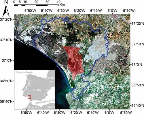
Usually, the highest monthly precipitation takes place in November and maximum inundation levels are reached during February. In late spring, marshes dry up slowly and most of their surface gets completely dry by the end of July (Green et al., 2016). Doñana, due to its strategic location between the continents of Europe and Africa, holds a high biodiversity reserve of European and Africa flora and fauna. Doñana marshes are breeding ground as well as a stopover point for birds moving between Europe and Africa, and host many species of migratory birds during the winter (Green et al., 2016; Kloskowski, Green, Polak, Bustamante, & Krogulec, 2009). Thus, water cycle information is of high importance for Doñana Protected Area managers to make decisions that balance bird nesting and cattle breeding ecosystem services, as expressed via the amount of biomass production due to water presence.

Satellite imagery

75 S1 Ground Range Detected (GRD) products, between 9 December 2015 and 14 July 2018, were downloaded from the Copernicus Open Access Hub. These products belong to the same 12-day repeat orbit cycle of S1A satellite. The Science Toolbox Exploitation Platform (SNAP) Toolkit, developed by ESA and distributed freely under the GNU GPL license, was used for S1 data pre-processing. The SNAP graph for the pre-processing was implemented with the support of Terradue (based in Rome, Italy), on their Ellip Cloud Computing environment, providing automated data processing, and systematic delivery of results to the ECOPOTENTIAL EO Data archive (Brito, Gonçalves, & Caumont, 2016). The graph sequentially applies pre-processing steps as follows: (i) radiometric calibration, (ii) speckle filtering using Lee filter with window size 3 × 3 and (iii) Range-Doppler Terrain Correction. Backscatter intensities were converted into decibel-scale (dB).

Reference date

A total of 42 inundation maps of the Doñana area for the period between 19 December 2015 and 16 July 2018, which are generated by the unsupervised approach upon S2 data as described in (Kordelas et al., 2018), are used in the training phase of the classification approach and for the evaluation of the S1-based generated inundation maps. Their accuracy is considered high enough to be used as the reference ground data. In particular, kappa coefficient for the complete buffered Biosphere Reserve area and the marshland wetland subarea (the study area in this work) is 0.8827 and 0.9413, respectively.

Methods

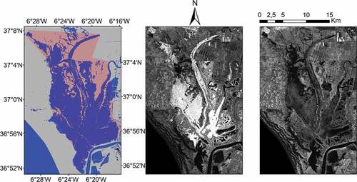
Clear water and emergent vegetation return diverse SAR backscatter, e.g. water returns low backscatter while emergent vegetation returns higher backscatter. During the training phase of a supervised approach, the use of pixels with diverse backscatter that are assigned to the same reference class may affect negatively the performance of the generated classification model. Figure 2 shows an example where it is evident that for the pixels classified as water in the S2 inundation map (Figure 2(a)) the vertically transmitted and vertically received (VV) and vertically transmitted and horizontally received (VH) polarisation values, as shown, respectively, in Figure 2(b,c), vary from very low to very high backscatter. This fact is more evident in the VV band. In order to suppress this problem, the introduced approach suggests pixel-centric multi-temporal classification instead of area-centric classification (as presented, for example at (Huang et al., 2018; Pham-Duc et al., 2017)).

Figure 2. (a) S2 inundation map on 02/04/2017 (with pale red over blue is denoted the marshland area), (b) VV and (c) VH polarization bands of S1 image on 02/04/2017.

Pixel-centric classification performs classification at a local but multi-temporal basis, and utilises in the training process multiple reference S2 inundation maps (and a swarm of S1 images, timely close to each one of them) that are distant in time to the target S1 data, for which there is interest to generate an inundation map (Figure 3). As a result numerous local classification models are applied; each one to the respective pixel, based on the location in the image. This is the approach examined in this study, whereas following ones are used for performance comparison: (a) area-centric classification that performs classification for the entire image utilising a single classification model and one S2 inundation map timely coinciding to the target S1 data (Figure 4); (b) simple thresholding that estimates thresholds on the intensity histograms of SAR bands, upon which the inundated areas are discriminated from the non-inundated ones (Figure 5).

Figure 3. Schematic flow diagram of the pixel centric classification approach.

Figure 4. Schematic flow diagram of the area centric classification approach.

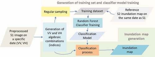
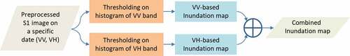
Figure 5. Schematic flow diagram of the simple thresholding approach.

Training dataset preparation for the pixel-centric classification

The training set is composed of 3 × 3 pixel samples, where each sample includes information about each pixel’s backscatter coefficient in the VV and VH polarisation bands of S1, algebraic combinations of VV and VH bands (as suggested in (Huang et al., 2018)), and the season of the year (Table 1), while the reference sample class for each pixel is derived from one or more S2 inundation maps at close temporal interval from the S1 data (less than 20 days). The meteorological season is defined according to the date of S1 acquisition as follows: “Winter” is the period from 1st December to 28th February (or 29th for leap years), “Spring” is from 1st March to 31st May, “Summer” is from 1st June to 31st August and “Autumn” is from 1st September to 30th November. More than one sample may correspond to a pixel, as the number of samples depends on the S1 images and the S2 reference maps to be taken into account according to the approach described below.

Table 1. Features used for classification training.

Feature	Equation	Reference
VH polarisation	${\sigma }_0^{\mathrm{V}\mathrm{H}}$
VV polarisation	${\sigma }_0^{\mathrm{V}\mathrm{V}}$
Polarised Ratio Index	${\sigma }_0^{\mathrm{V}\mathrm{H}}/{\sigma }_0^{\mathrm{V}\mathrm{V}}$	Brisco, Kapfer, Hirose, Tedford, & Liu, 2011
Normalised Difference Polarised Index (NDPI)	$\left({\sigma }_0^{\mathrm{V}\mathrm{V}}-{\sigma }_0^{\mathrm{V}\mathrm{H}}\right)/\left({\sigma }_0^{\mathrm{V}\mathrm{V}}+{\sigma }_0^{\mathrm{V}\mathrm{H}}\right)$	Mitchard et al., 2012
Normalized VH Index (NDHI)	${\sigma }_0^{\mathrm{V}\mathrm{H}}/\left({\sigma }_0^{\mathrm{V}\mathrm{V}}+{\sigma }_0^{\mathrm{V}\mathrm{H}}\right)$	McNairn & Brisco, 2004
Normalized VV Index (NVVI)	${\sigma }_0^{\mathrm{V}\mathrm{V}}/\left({\sigma }_0^{\mathrm{V}\mathrm{V}}+{\sigma }_0^{\mathrm{V}\mathrm{H}}\right)$	McNairn & Brisco, 2004
Meteorological season	(winter, spring, summer, autumn)

Two different cases were examined for generating the training sets (Figure 3): (a) in the first case, abbreviated as TIM, two S2 ground truth inundation maps, one of them preceding and the other one following the date of target S1 image, and their timely close S1 images, are used to train local RF models used for the classification of the S1 target image, and (b) in the second case, abbreviated as GRP, a group of S2 ground truth inundation maps, where half of the maps precede chronologically the date of target S1 image and the rest of them follow this date, and their timely close S1 images, are used for the classification of the S1 target image. In case of TIM, S2 maps are selected based on the following four subcases: (i) the closest before and the closest after the target date, i.e. TIM-1, (ii) the second closest before and the second closest after the target date, i.e. TIM-2, (iii) the third closest before and the third closest after the target date, i.e. TIM-3 and (iv) the fourth closest before and the fourth closest after the target date, i.e. TIM-4. In case of GRP, S2 maps are selected based on the following four subcases: (i) the closest before and the closest after the target date, i.e. GRP-1, (ii) the combination of the two closest before and the combination of the two closest after the target date, i.e. GRP-2, (iii) the combination of the three closest before and the combination of the three closest after the target date, i.e. GRP3 and (iv) the combination of the four closest before and the combination of the four closest after the target date, i.e. GRP-4.

Key to the formation of the training dataset for both TIM and GRP is the implementation of the approach for the time proximity of S1 data to the S2-derived reference maps. S1 image shall not be timely further away more than 20 days (less than 2 orbit overpasses of S1A away) from the S2 reference map, otherwise the S1 image is not utilised. If the S1 image is timely close to more than one S2 maps, then the class assignment per pixel follows the one of the closest preceding S2 map, provided that following ruleset is satisfied:

• If the closest preceding S2 date has Da days difference in relation to the S1 image and the closest following S2 date has Db days difference in relation to the S1 image, and the absolute value of (Da/(Da + Db) – Db/(Da + Db)) is bigger than 0.15 (i.e. more than 5 days out of 35 days of aggregated time interval between the preceding and the following date; keeping the aforementioned condition for the S1A data take to remain timely away no more than 20 days from the S2 reference map), and

• Da<Db,

then it is assumed that the class can be derived reliably from the closest preceding S2 map. If the last rule of the ruleset is Da > Db instead of Da < Db, then the class is derived from the closest following S2 map. If the aforementioned ruleset is not satisfied then the pixel class is the one corresponding to the one appearing in the majority of the timely close S2 maps (less than 20 days). If no majority is evident, then the pixel sample is not taken into consideration.

As a result, multiple training datasets are created for non-overlapping windows of 3 × 3 pixels by combining the respective samples.

Training dataset preparation for the area-centric classification

The sampling of the points on the S1 image is regular, and one per three pixels is sampled for the inundation class, while one per nine pixels is sampled for the non-inundation class. Pixels classes are derived from the S2 inundation map that is overlaid on the S1 image. The sampling interval is chosen this way to keep a balance in the sample numbers, because of the usual lesser extent covered by the inundated pixels in the study area. The same sampling frequency is applied to both horizontal and vertical axes. Per sample point, the features given in Table 1 are estimated, and the class is derived from the S2 inundation map. Provided that the acquisition date of S1 coincides with the date of the S2 inundation map, it is ensured that the sample class can be reliably derived. In this way, a training set is generated for a specific date (Figure 4).

Contrary to the training dataset preparation of the pixel-centric classification approach under investigation, in this approach there is one training dataset derived from the complete image, and no multiple datasets derived from small windows. At the same time, the S2 inundation map used as reference map timely overlaps to the S1 image and no multiple S2 inundation maps are used.

Random Forest classification

Pixel-centric classification

Sets of training samples are used to train one local RF classifier per small image subset corresponding to pixel windows of size 3 × 3. The number of the RF trees is set to 128. A fivefold cross validation repeated three times is performed in order to limit and reduce overfitting on the training set. The RF model estimated per subset is applied to the features estimated for the pixels of this subset on the target S1 image in order to classify the product into inundated and non-inundated areas.

Area-centric classification

The training set is used to train a RF classifier for a specific date, using the same RF training parameters described in the previous paragraph. The resulting RF model is applied to the features calculated for the pixels of the S1 image acquired at the same date, in order to classify the image into inundated and non-inundated areas.

Simple thresholding approach

This approach relies on the estimation of thresholds on the histograms of the VV and VH bands. A threshold is detected on the first deep valley of the histogram, so as to separate low-intensity areas that most probably correspond to inundated area from areas with higher backscatter intensity. This way VV-based and VH-based inundation maps are generated. A combined inundation map is generated by denoting that an area is inundated if it is inundated in both VV-based and VH-based maps, otherwise it is denoted as non-inundated (Figure 5).

Accuracy assessment of the complete inundations maps generated via the pixel-centric classification, area-centric classification and simple thresholding approaches, is performed for eight different dates where S1 and S2 acquisition days coincide (see Table 2). For the experiments evaluating the pixel-centric classification approach, S1 and S2 data coinciding on each of eight different dates were excluded from the formation of the training datasets in order to avoid bias of the accuracy estimation results. On the other hand, for the area-centric classification approach, S1 and S2 data coinciding on the same date were used for the formation of the training datasets.

Table 2. Dates of coinciding S1 and S2 acquisition. Green colour highlights the presence of emergent vegetation covering the marshland area.

Reference dates
06/06/2016	05/08/2016	04/10/2016	02/04/2017	01/06/2017	31/07/2017	27/01/2018	28/03/2018

Results

Accuracy assessment for TIP and GRP cases of pixel-centric classification

The accuracy estimation results include the kappa coefficient (k). k < 0 is indicating no agreement, 0–0.20 as slight, 0.21–0.40 as fair, 0.41–0.60 as moderate, 0.61–0.80 as substantial and 0.81–1 as almost perfect agreement between the observed and predicted classes (Landis & Koch, 1977).

Classification was performed for the TIM and GRP cases and the k results are presented in Figures 6 and 7, for the two cases, respectively. The x axis in both figures is the mean day difference (mdd) between the S1 inundation map and the S2 inundation maps, which are used as ground reference. The different subcases of the TIM (TIM-1 to TIM-4) or GRP (GRP-1 to GRP-4) cases are depicted with markers of different shape and color.

Figure 6. Kappa of four different pairs in relation with the Mean Day Difference of the S2 reference map to the S1 target date (TIM case).

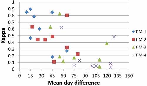
TIM case results show that when mdd is below 30 days, k is over 0.4 and its average value is 0.6664. Between 30 and 70 mdd, more than half of the examined pairs have k over 0.4 and its average value is 0.4294, while after 70 mdd, k is below 0.4 for all of the pairs, except for one. It is evident that the closest are the S2 maps to the S1 data the higher is the value of k.

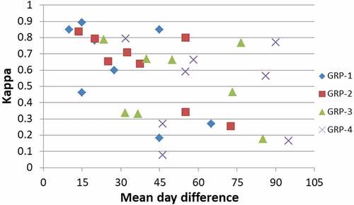
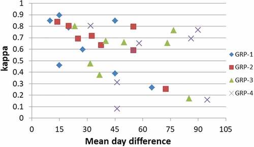
GRP results show that k is evidently much higher than 0.4 in all groups when mdd is below 30 and its average value is 0.7399. When mdd is between 30 and 70 mdd k is over 0.4 for more than half of the groups and its average value is 0.5112. Same situation reveals over 70 mdd with an average value of 0.4514. From the observation of the points corresponding to each group, it can be concluded that it is preferable to have more than one training dates considered but these shall be at the same time the closer possible to the target S1 date.

The comparison between Figures 6 and 7 shows that the results of GRP case outperform these of TIM case. Therefore, the incorporation of multiple S2 maps in the process assists in increasing k and consequently the credibility of the result.

Figure 7. Kappa of four different groups in relation with the Mean Day Difference of the S2 reference map to the S1 target date (GRP case).

Minimisation of the classification speckle effect

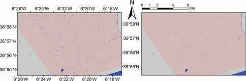
Since the classification is performed locally for small windows, some misclassified outcomes may appear. In order to examine their influence on the result, inundated objects up to 10 pixels are switched to the non-inundated class. Figure 8 depicts a sub-set of the inundation map generated on 04/10/2016 for GRP case, GRP-2. The comparison between Figure 8(a,b), shows that spurious inundated pixels have been efficiently removed from the inundation map. From the quantitative perspective, k increases from 0.3414 to 0.5917 after this speckle effect minimisation.

Figure 8. Inundation map on 04/10/2016 for GRP case, GRP-2, (a) before noise removal, (b) after noise removal. Water and dry areas are denoted with blue and gray, respectively, and with pale red is denoted the marshland area.

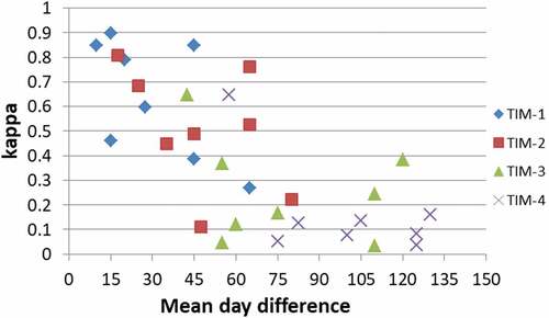
Following the minimisation of the classification speckle effect for the TIM case (Figure 9) results show that k is over 0.6 when mdd is below 30 days, with the exception of one pair, and its average value is 0.7264, while before the speckle effect minimisation k value was over 0.4 and on average 0.6664, respectively. Between 30 and 70 mdd, about half of the points have k over 0.4 and an average value is 0.4360, showing no significant change against the original result. After 70 mdd, k is below 0.4 for all of the points. On average, k increases about 0.0081 after possible misclassification cases were minimised.

Figure 9. Kappa of four different pairs (TIM case) in relation with the Mean Day Difference of the S2 reference map to the S1 target date, after taking into consideration possible misclassified outcomes.

The classification results for the GRP case (Figure 10) show that k is over 0.6 when mdd is below 30, with the exception of one experiment, and its average value is about 0.7479, while before speckle effect minimisation average k value was 0.7399. At the same time, when mdd is between 30 and 70 mdd k is over 0.6 for most of the experiments and average k is 0.5546, while before speckle effect minimisation k value was over 0.4 and on average 0.5112, respectively. After mdd 70, k still varies significantly from low to high values, but for most of the experiments k is over 0.6 after the speckle effect minimisation, while prior its application most of the experiments had a k below 0.6. On average, k increases by 0.03347 after possible misclassification cases were minimised.

Figure 10. Kappa of four different groups (GRP case) in relation with the Mean Day Difference of the S2 reference map to the S1 target date, after taking into consideration possible misclassified outcomes.

Pixel-centric classification compared to area-centric classification and simple thresholding

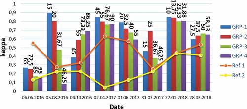
Figures 11 and 12 demonstrate the classification results for TIM and GRP cases after speckle effect minimisation, respectively, against the area-centric reference classification (referred to also as “Ref. 1”) and simple thresholding (referred to also as “Ref. 2”). Each clustered column corresponds to a date and the examined pairs or groups per date. Each point of each line corresponds to the kappa result of the area-centric reference classification or simple thresholding for each date. Specifically, for the latter approach, VV-based, VH-based and combined inundation maps of a date are separately evaluated for their accuracy and the highest k is the final result presented for this date, as results vary significantly due to the variable backscatter response in VV and VH (Figure 2). The numbers appearing on top of the columns of Figures 11 and 12, correspond to the mdd values of the experiments performed for the TIM and GRP cases, respectively.

Figure 11. Kappa of TIM case per date and pair after classification speckle effect minimization, given in clustered columns; kappa of the area centric reference classification given as orange line with markers (referred to as ‘Ref.1’); and kappa of the simple thresholding given as yellow line with markers (referred to as ‘Ref.2’). The mdd value of each date and pair is given on top of the corresponding column indicating kappa.

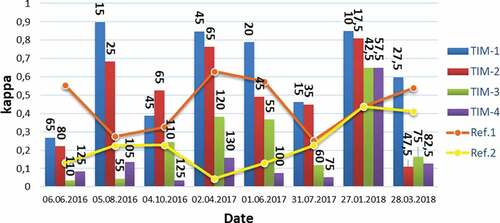
Figure 12. Kappa of GRP case per date and group after classification speckle effect minimization, given in clustered columns; kappa of the area centric reference classification given as line with markers (referred to as ‘Ref.1’); and kappa of the simple thresholding given as yellow line with markers (referred to as ‘Ref.2’). The mdd value of each date and group is given on top of the corresponding column indicating kappa.

The results of Figure 11 show that on 06/06/2016, k is lower for all pairs compared to Ref. 1. For the rest of the dates, k of TIM-1 and TIM-2 is higher than k of Ref. 1 and Ref. 2, with the exception of 28/03/2018, where k of TIM-2 is lower than k of Ref. 1 and Ref. 2. k for TIM-3 is lower than Ref. 1 for six out of eight dates and lower than Ref. 2 for four out of eight dates, and k for TIM-4 is lower than Ref. 1 for seven out of eight dates and lower than Ref. 2 for six out of eight dates. Figure 11 also shows that for each date, TIM-1 has higher k than the rest of the pairs, with the exception of 04/10/2016, where k for TIM-2 is higher than the one for TIM-1. Also, the trend is that when moving from TIM-1 to TIM-4, and as mdd increases, k decreases significantly. In particular, average k for TIM-1, TIM-2, TIM-3, TIM-4 is 0.6371, 0.5063, 0.2508, 0.1643, respectively, whereas average k for the area-centric reference classification and simple thresholding is 0.449 and 0.2292, respectively.

The results of Figure 12 show that on 06/06/2016, k is lower for all groups compared to Ref. 1. This is probably related to the mdd values of all groups on 06/06/2016, which are significantly higher than the mdd values of the respective groups on other dates. For the rest of the dates, k of GRP-1, GRP-2, GRP-3 and GRP-4 is higher than k of Ref. 1 and Ref. 2, with the exception of 05/08/2016, where k of GRP-4 is lower than k of Ref. 1 and Ref. 2. Average k for groups GRP-1, GRP-2, GRP-3, GRP-4 is 0.6371, 0.6658, 0.5722, 0.5074, respectively, whereas average k for the area-centric reference classification and simple thresholding is 0.449 and 0.2292, respectively.

Supplementary material I in Annex 1, Annex 2, Annex 3 provides information on the confusion matrices of the experiments performed to estimate k results presented in Figures 6, 7 and 9–12. Supplementary material II shows several examples of inundation maps considered in the accuracy assessment.

Discussion

In this study the relative value changes of a pixel in time are considered indicative for the situation on the ground (e.g. x to x’ backscatter coefficient change means for this specific pixel the transition from the non-inundated to inundated condition) rather than the pixel absolute value pairing with a specific state (e.g. x backscatter coefficient means inundation for all pixels). As such, for example, it is considered that a higher backscatter, which may have excluded a pixel from assigning it to the inundation class according to the thresholding approach result, may still lead the classification process to assign it to the inundation class. It is assumed that an area could show a different backscatter temporal signature than another one, even if similar inundation states are present. Water depth (Kasischke et al., 2009), water surface roughness (Bolanos et al., 2016; Martinis et al., 2015; Marti-Cardona et al., 2013), emergent vegetation from time to time at different intensity (Huang et al., 2018), landscape features in relation with the SAR incidence angle (Bolanos et al., 2016; White, Brisco, Dabboor, Schmitt, & Pratt, 2015), among others, may influence the backscatter intensity in a way that a grey value here may be related to the same ground state with a darker or a lighter value elsewhere. The changes of the backscatter through time may also vary with a different pace for similar developing influencing phenomena (e.g. inundation).

The pixel-centric approach presented in this study manages, as shown from the results, to capture this pixel-related backscatter fluctuation in time, train local RF classification models, and achieve credible for the user results. Comparison results of the pixel-centric classification against the area-centric one confirm that the accuracy of the former classification is superior. Additionally, based on the comparison between pixel-centric classification and simple thresholding, it is expected that the suggested classification approach will outperform thresholding approaches, e.g. (Li & Wang, 2015; Martinis et al., 2009; Nakmuenwai et al., 2017), attempting to estimate thresholds on SAR intensity histograms, in order discriminate low from high backscatter areas. Moreover, the suggested approach requires for no auxiliary data, which is a prerequisite for (Hahmann & Wessel, 2010; Mason et al., 2007; Pierdicca et al., 2013; Sui et al., 2018; Marti-Cardona et al., 2013), or any manual intervention that is necessary in several approaches relying on contour models, e.g. (Hahmann & Wessel, 2010).

Next and main research step for this study was to identify its constraints towards its operational application. The performance of the approach depends on the availability of S2 inundation maps at close temporal proximity to the target S1 image. Experiments have shown that high classification accuracy can be achieved when mdd between target S1 image and available S2 maps is below 30. This means that the suggested approach can be reliably used even if the cloud conditions last for up to six sequential S2 data takes, bearing in mind that S2 revisit time is 5 days. When mdd overcomes 30, the maintenance of high accuracy becomes doubtful for an operational use. The experiments also confirm that accuracy may vary for different dates even if considering the same case and subcase and similar mdd. For example, according to Figure 12, for GRP-2 on 04/10/2016 and 02/04/2017, k is 0.3878 and 0.8474, respectively, for the same mdd:55, and for GRP-4 on 05/08/2016 and 31/07/2017, k is 0.0783 and 0.4613, respectively, for the same mdd: 46.25.

Given that S2 inundation maps are used as reference for the training of local classifiers, possible classification errors in the S2 inundation maps will lead to erroneous classifications in S1-derived inundation maps. Moreover, the two cases adopted for generating training samples per S1 product that is close to one or more S2 reference inundation maps, introduce a degree of uncertainty in the definition of the reference classes. This is because it is not completely certain that the real class of a pixel on the S1 image coincides to the class assigned based on its close S2 inundation maps, bearing in mind that the acquisition date of S1 image most possibly will not coincide with the dates of S2 maps.

Regarding the computational cost, the pixel- and area-centric classification approaches require much more time compared to the thresholding one, considering that (a) for the pixel-centric classification the number of training pixels per 3 × 3 pixels window and for the eight dates considered in the accuracy assessment varies from 27 to 63 for the TIM case and from 27 to 144 for the GRP case; and (b) for the area-centric classification the average number of training points for the eight dates considered in the accuracy assessment is 100143. However, the cost of the pixel-centric classification can be minimised, since multiple datasets of non-overlapping 3 × 3 windows can be trained in parallel using multiple cores. On the contrary, the training dataset of the area-centric classification, which is takes into account the entire image at once should be executed in a single core.

Application of the introduced supervised method to additional study areas shall examine its credibility towards method transferability to other locations and biogeographical zones. Widely applicable hydrological models could be also used complementary with S1 and S2 inundation maps to fill in inundation mapping gaps for prolonged periods of cloud coverage; thus, allowing for finer monitoring of the temporal variability of the hydrological cycle.

Conclusion

This study presents a pixel-centric classification approach for estimating inundation maps in the Doñana marshland fusing S1 data and S2-derived inundation maps. The methodology relies on multiple local RF classification models trained with samples formed by S1-based features and S2 inundation map classes. TIM and GRP cases were examined for the formation of training samples. The evaluation results indicated that an inundation map can be generated for a target S1 image with high accuracy, when mdd between the date of the target S1 image and the dates of the S2 inundation maps are below 30 days, i.e. average kappa is 0.6664 and 0.7479 for the TIM and GRP cases, respectively. Beyond this result and without considering the mdd threshold of 30 days, the GRP-2 subcase outperformed all others with an average classification accuracy of 0.6658. The comparison of the pixel-centric classification approach against area-centric and thresholding approaches shows overall higher performance for the pixel-centric one. In particular, the best kappa achieved via the area-centric approach is 0.6658, while for the area centric and thresholding approaches is 0.449 and 0.2292, respectively.

In the future, the suggested approach could be applied to other wetland areas to examine transferability of the approach and limitations. The utilisation of ancillary information, such as the DEM, may further correct for erroneous classifications. Additionally, alternative post-processing techniques could be examined for the removal of small objects erroneously denoted as inundated.

Once verified at more areas and transformed into an operational tool, this study’s approach may support Protected Areas managers and personnel—at least—towards finer data-driven decisions, as the influence of non-favourable atmospheric conditions on the availability of monitoring data may be minimised. Latter shall be advantageous in tropical areas or areas at higher latitudes.

Acknowledgments

This study is supported and funded by the European Union’s Horizon 2020 research and innovation programme under grant agreement No 641762, ECOPOTENTIAL. We gratefully acknowledge the support of Fabrice Brito (Terradue Srl) for the provision of pre-processed S1 data delivered via the EO Data Processing tools (Terradue‘s Ellip Workflows solution) of ECOPOTENTIAL project.

Disclosure statement

No potential conflict of interest was reported by the authors.

Supplementary material

Supplemental data for this article can be accessed here.

Correction Statement

This article has been republished with minor changes. These changes do not impact the academic content of the article.

Additional information

Funding

This work was supported partially by the European Union’s Horizon 2020 ECOPOTENTIAL RIA project [641762], and partially by EARSeL.

References

- Arnesen, A.S., Silva, T.S., Hess, L.L., Novo, E.M., Rudorff, C.M., Chapman, B.D., & McDonald, K.C. (2013). Monitoring flood extent in the lower Amazon River floodplain using ALOS/PALSAR ScanSAR images. Remote Sensing of Environment, 130, 51–61. doi:10.1016/j.rse.2012.10.035
- Beatty, W.S., Kesler, D.C., Webb, E.B., Raedeke, A.H., Naylor, L.W., & Humburg, D.D. (2014). The role of protected area wetlands in waterfowl habitat conservation: Implications for protected area network design. Biological Conservation, 176, 144–152. doi:10.1016/j.biocon.2014.05.018
- Behnamian, A., Banks, S., White, L., Brisco, B., Milard, K., Pasher, J., … Battaglia, M. (2017). Semi-automated surface water detection with synthetic aperture radar data: A Wetland case study. Remote Sensing, 9(12), 1209. doi:10.3390/rs9121209
- Bolanos, S., Stiff, D., Brisco, B., & Pietroniro, A. (2016). Operational surface water detection and monitoring using Radarsat 2. Remote Sensing, 8(4), 285. doi:10.3390/rs8040285
- Bovolo, F., & Bruzzone, L. (2007). A split-based approach to unsupervised change detection in large-size multitemporal images: Application to tsunami-damage assessment. IEEE Transactions on Geoscience and Remote Sensing, 45(6), 1658–1670. doi:10.1109/TGRS.2007.895835
- Brisco, B., Kapfer, M., Hirose, T., Tedford, B., & Liu, J. (2011). Evaluation of C-band polarization diversity and polarimetry for wetland mapping. Canadian Journal of Remote Sensing, 37(1), 82–92. doi:10.5589/m11-017
- Brito, F., Gonçalves, P., & Caumont, H. (2016). EO data processing tools v1 (Deliverable No: 3.2), ECOPOTENTIAL H2020 EU project (pp. 87).
- Chapman, B., McDonald, K., Shimada, M., Rosenqvist, A., Schroeder, R., & Hess, L. (2015). Mapping regional inundation with spaceborne L-Band SAR. Remote Sensing, 7(5), 5440–5470. doi:10.3390/rs70505440
- Díaz-Delgado, R., Aragonés, D., Afán, I., & Bustamante, J. (2016). Long-term monitoring of the flooding regime and hydroperiod of Doñana marshes with Landsat time series (1974–2014). Remote Sensing, 8(9), 775. doi:10.3390/rs8090775
- Donchyts, G., Schellekens, J., Winsemius, H., Eisemann, E., & van de Giesen, N. (2016). A 30 m resolution surface water mask including estimation of positional and thematic differences using landsat 8, srtm and openstreetmap: A case study in the Murray-Darling Basin, Australia. Remote Sensing, 8(5), 386. doi:10.3390/rs8050386
- Du, Y., Zhang, Y., Ling, F., Wang, Q., Li, W., & Li, X. (2016). Water bodies’ mapping from Sentinel-2 imagery with modified normalized difference water index at 10-m spatial resolution produced by sharpening the SWIR band. Remote Sensing, 8(4), 354. doi:10.3390/rs8040354
- Feng, Q., Gong, J., Liu, J., & Li, Y. (2015). Flood mapping based on multiple endmember spectral mixture analysis and random forest classifier—The case of Yuyao, China. Remote Sensing, 7(9), 12539–12562. doi:10.3390/rs70912539
- Giustarini, L., Chini, M., Hostache, R., Pappenberger, F., & Matgen, P. (2015). Flood hazard mapping combining hydrodynamic modeling and multi annual remote sensing data. Remote Sensing, 7(10), 14200–14226. doi:10.3390/rs71014200
- Green, A.J., Bustamante, J., Janss, G.F.E., Fernández-Zamudio, R., & Díaz-Paniagua, C. (2016). Doñana Wetlands (Spain). In Finlayson C., Milton G., Prentice R., Davidson N. (eds), The Wetland book (pp. 1–14). Dordrecht: Springer.
- Gstaiger, V., Huth, J., Gebhardt, S., Wehrmann, T., & Kuenzer, C. (2012). Multi-sensoral and automated derivation of inundated areas using TerraSAR-X and ENVISAT ASAR data. International Journal of Remote Sensing, 33(22), 7291–7304. doi:10.1080/01431161.2012.700421
- Guo, M., Li, J., Sheng, C., Xu, J., & Wu, L. (2017). A review of wetland remote sensing. Sensors, 17(4), 777. doi:10.3390/s17050968
- Hahmann, T., & Wessel, B. (2010, June). Surface water body detection in high-resolution TerraSAR-X data using active contour models. In Synthetic Aperture Radar (EUSAR), 2010 8th European conference on (pp. 1–4), Aachen, Germany, 7−10 June 2010.
- Henry, J.B., Chastanet, P., Fellah, K., & Desnos, Y.L. (2006). Envisat multi‐polarized ASAR data for flood mapping. International Journal of Remote Sensing, 27(10), 1921–1929. doi:10.1080/01431160500486724
- Huang, W., DeVries, B., Huang, C., Lang, M.W., Jones, J.W., Creed, I.F., & Carroll, M.L. (2018). Automated extraction of surface water extent from Sentinel-1 data. Remote Sensing, 10(5), 797. doi:10.3390/rs10050797
- Irwin, K., Beaulne, D., Braun, A., & Fotopoulos, G. (2017). Fusion of SAR, optical imagery and airborne LiDAR for surface water detection. Remote Sensing, 9(9), 890. doi:10.3390/rs9090890
- Kasischke, E.S., Bourgeau-Chavez, L.L., Rober, A.R., Wyatt, K.H., Waddington, J.M., & Turetsky, M.R. (2009). Effects of soil moisture and water depth on ERS SAR backscatter measurements from an Alaskan wetland complex. Remote Sensing of Environment, 113, 1868–1873. doi:10.1016/j.rse.2009.04.006
- Khan, S.I., Hong, Y., Wang, J., Yilmaz, K.K., Gourley, J.J., Adler, R.F., … Irwin, D. (2011). Satellite remote sensing and hydrologic modeling for flood inundation mapping in Lake Victoria basin: Implications for hydrologic prediction in ungauged basins. IEEE Transactions on Geoscience and Remote Sensing, 49(1), 85–95. doi:10.1109/TGRS.2010.2057513
- Kloskowski, J., Green, A.J., Polak, M., Bustamante, J., & Krogulec, J. (2009). Complementary use of natural and artificial wetlands by waterbirds wintering in Doñana, south-west Spain. Aquatic Conservation: Marine and Freshwater Ecosystems, 19(7), 815–826. doi:10.1002/aqc.v19:7
- Ko, B.C., Kim, H.H., & Nam, J.Y. (2015). Classification of potential water bodies using Landsat 8 OLI and a combination of two boosted random forest classifiers. Sensors, 15(6), 13763–13777. doi:10.3390/s150613763
- Kordelas, G., Manakos, I., Aragonés, D., Díaz-Delgado, R., & Bustamante, J. (2018). Fast and automatic data-driven thresholding for inundation mapping with Sentinel-2 data. Remote Sensing, 10(6), 910. doi:10.3390/rs10060910
- Landis, J.R., & Koch, G.G. (1977). The measurement of observer agreement for categorical data. Biometrics, 159–174. doi:10.2307/2529310
- Li, J., & Wang, S. (2015). An automatic method for mapping inland surface waterbodies with Radarsat-2 imagery. International Journal of Remote Sensing, 36(5), 1367–1384. doi:10.1080/01431161.2015.1009653
- Marti-Cardona, B., Dolz-Ripolles, J., Lopez-Martinez, C. (2013). Wetland inundation monitoring by the synergistic use of ENVISAT/ASAR imagery and ancilliary spatial data. Remote sensing of environment, 139, 171–184. doi:10.1016/j.rse.2013.07.028
- Martinis, S., Kuenzer, C., Wendleder, A., Huth, J., Twele, A., Roth, A., & Dech, S. (2015). Comparing four operational SAR-based water and flood detection approaches. International Journal of Remote Sensing, 36(13), 3519–3543. doi:10.1080/01431161.2015.1060647
- Martinis, S., Twele, A., & Voigt, S. (2009). Towards operational near real-time flood detection using a split-based automatic thresholding procedure on high resolution TerraSAR-X data. Natural Hazards and Earth System Sciences, 9(2), 303–314. doi:10.5194/nhess-9-303-2009
- Martinis, S., Twele, A., & Voigt, S. (2011). Unsupervised extraction of flood-induced backscatter changes in SAR dat` using Markov image modeling on irregular graphs. IEEE Transactions on Geoscience and Remote Sensing, 49(1), 251–263. doi:10.1109/TGRS.2010.2052816
- Mason, D.C., Horritt, M.S., Dall‘Amico, J.T., Scott, T.R., & Bates, P.D. (2007). Improving river flood extent delineation from synthetic aperture radar using airborne laser altimetry. IEEE Transactions on Geoscience and Remote Sensing, 45(12), 3932–3943. doi:10.1109/TGRS.2007.901032
- McNairn, H., & Brisco, B. (2004). The application of C-band polarimetric SAR for agriculture: A review. Canadian Journal of Remote Sensing, 30(3), 525–542. doi:10.5589/m03-069
- Mitchard, E.T., Saatchi, S.S., White, L., Abernethy, K., Jeffery, K.J., Lewis, S.L., … Meir, P. (2012). Mapping tropical forest biomass with radar and spaceborne LiDAR in Lopé National Park, Gabon: Overcoming problems of high biomass and persistent cloud. Biogeosciences, 9(1), 179–191. doi:10.5194/bg-9-179-2012
- Musamba, E.B., Boon, E.K., Ngaga, Y.M., Giliba, R.A., & Dumulinyi, T. (2012). The recreational value of Wetlands: Activities, socio-economic activities and consumers’ surplus around Lake Victoria in Musoma Municipality, Tanzania. Journal of Human Ecology, 37(2), 85–92. doi:10.1080/09709274.2012.11906451
- Nakmuenwai, P., Yamazaki, F., & Liu, W. (2017). Automated extraction of inundated areas from multi-temporal dual-polarization RADARSAT-2 images of the 2011 central Thailand flood. Remote Sensing, 9(1), 78. doi:10.3390/rs9010078
- Nandi, I., Srivastava, P.K., & Shah, K. (2017). Floodplain mapping through support vector machine and optical/infrared images from Landsat 8 OLI/TIRS sensors: Case study from Varanasi. Water Resources Management, 31(4), 1157–1171. doi:10.1007/s11269-017-1568-y
- Park, E., Lee, S., & Peters, D.J. (2017). Iowa wetlands outdoor recreation visitors’ decision-making process: An extended model of goal-directed behavior. Journal of Outdoor Recreation and Tourism, 17, 64–76. doi:10.1016/j.jort.2017.01.001
- Pham-Duc, B., Prigent, C., & Aires, F. (2017). Surface water monitoring within Cambodia and the Vietnamese Mekong Delta over a year, with Sentinel-1 SAR observations. Water, 9(6), 366. doi:10.3390/w9060366
- Pierdicca, N., Pulvirenti, L., Chini, M., Guerriero, L., & Candela, L. (2013). Observing floods from space: Experience gained from COSMO-SkyMed observations. Acta astronautica, 84, 122–133. doi:10.1016/j.actaastro.2012.10.034
- Ramos-Fuertes, A., Marti-Cardona, B., Bladé, E., & Dolz, J. (2014). Envisat/ASAR images for the calibration of wind drag action in the Doñana wetlands 2D hydrodynamic model. Remote Sensing, 6(1), 379–406. doi:10.3390/rs6010379
- Sarp, G., & Ozcelik, M. (2017). Water body extraction and change detection using time series: A case study of Lake Burdur, Turkey. Journal of Taibah University for Science, 11(3), 381–391. doi:10.1016/j.jtusci.2016.04.005
- Skakun, S. (2012). A neural network approach to flood mapping using satellite imagery. Computing and Informatics, 29(6), 1013–1024.
- Sui, H., An, K., Xu, C., Liu, J., & Feng, W. (2018). Flood detection in PolSAR images based on level set method considering prior geoinformation. IEEE Geoscience and Remote Sensing Letters, 15(5), 699–703. doi:10.1109/LGRS.2018.2810122
- Sun, F., Sun, W., Chen, J., & Gong, P. (2012). Comparison and improvement of methods for identifying waterbodies in remotely sensed imagery. International Journal of Remote Sensing, 33(21), 6854–6875. doi:10.1080/01431161.2012.692829
- Wang, Y., & Yésou, H. (2018). Remote sensing of floodpath Lakes and Wetlands: A challenging frontier in the monitoring of changing environments. Remote Sensing, 10(12), 1955. doi:10.3390/rs10121955
- White, L., Brisco, B., Dabboor, M., Schmitt, A., & Pratt, A. (2015). A collection of SAR methodologies for monitoring wetlands. Remote Sensing, 7(6), 7615–7645. doi:10.3390/rs70607615
- Yang, X., & Lu, X.X. (2013). Delineation of lakes and reservoirs in large river basins: An example of the Yangtze River Basin, China. Geomorphology, 190, 92–102. doi:10.1016/j.geomorph.2013.02.018
- Zhang, L., Wang, M.H., Hu, J., & Ho, Y.S. (2010). A review of published wetland research, 1991–2008: Ecological engineering and ecosystem restoration. Ecological Engineering, 36(8), 973–980. doi:10.1016/j.ecoleng.2010.04.029