Nonlinear unmixing of minerals based on the log and continuum removal model

ABSTRACT

Spectral mixing models for minerals can be complex, and choosing the right unmixing model is indispensable to ensure the accuracy of spectral unmixing. Continuum removal (CR) and natural log operation have the potential to eliminate nonlinear effects in spectral mixing, and have already been used in nonlinear spectral unmixing applications. In this study, the newly proposed log and CR (LCR) model and four other spectral unmixing models for mineral analysis (the linear model, CR model, natural log model, and simplified Hapke model) were summarized and applied to both laboratory mineral powder spectra and hyperspectral data of Cuprite, Nevada, USA. This paper summarizes the concept of mixing reflectance reconstruction (MRR), along with a comprehensive method to determine accuracy based on MRR results, which can be performed in different dimensions, such as spatial dimension and spectral dimension. The LCR model performed the best in both laboratory experiments and image data analysis, indicating its strong potential for practical application. The level of atmospheric correction’s influence on unmixing accuracy varied for different spectral unmixing models, among which LCR model also had the best performance.

KEYWORDS:

• Spectral unmixing
• hyperspectral data
• continuum removal
• natural-log operation
• mineral mapping

Introduction

In laboratory research, reflectance spectra of many minerals have been examined (Adams, 1974; Hunt, 1977), but natural surfaces are commonly composed of a set of intimately mixed minerals and alteration products (Mustard & Pieters, 1987). Although hyperspectral data have been successfully used for mineral detection (Brandmeier, Erasmi, & Hansen, 2013; Clark, Swayze, & Livo, 2003; Meer, Werff, & Ruitenbeek, 2012), mineral abundance is difficult to retrieve. The retrieval of mineral abundances is hindered by the complexities of mineral spectra due to the mixture characteristics.

Spectral unmixing is an effective tool for retrieving mineral abundance using hyperspectral data, which decomposes a mixed pixel into a collection of constituents, or endmembers. This involves the extraction of endmember spectra and the estimation of abundance values (Chen, Richard, & Honeine, 2013). In geological remote sensing, spectral unmixing can be utilized to achieve the precise abundance and distribution of minerals, which is acquired from satellite data, airborne data, field data, or core data (Van der Meer, van der Werff, & van Ruitenbeek, 2012; Zhao, Zhang, Wu 2013).

Depending on the hyperspectral image under study, mixing models for spectral mixtures can be linear or nonlinear, and the linear mixing model (LMM) is most commonly used model (Halimi, Altmann, & Dobigeon, 2011). Spectral unmixing models can generally be divided into two categories: linear unmixing models based on LMM and nonlinear unmixing models (Ichoku & Karnieli, 1996). As the most widely used model, LMM has abundant applications in mineral analysis (Li, Fang, & Zhou, 2014; Schmidt, Legendre, & Le Mouëlic, 2014; Zhang, Rivard, & Sanchez-Azofeifa, 2004). When nonlinear effects are strong, they can affect the accuracy of spectral unmixing based on the LMM (Hapke, 1981; Nascimento & Bioucas-Dias, 2010). Therefore, the mixing model for minerals tends to be more complicated, and it is necessary to select a suitable spectral unmixing model before conducting mineral spectral unmixing.

In nonlinear unmixing models, linearization based on a reasonable physical model is a commonly used approach to eliminate nonlinear effects, so the pre-processed data can be handled in the same way as in a linear unmixing model. Another approach used in nonlinear unmixing models is to perform nonlinear unmixing on original reflectance data directly, such as bilinear methods, kernel-based methods, neural networks, etc. (Halimi et al., 2011; Haykin, 2009; Heylen & Gader, 2014). In this study, the principle issues are the physical mechanism and the reversibility of spectral unmixing models, and the models using the first approach will be discussed. One of the most representative nonlinear models for minerals is the classical radiative transfer model (Hapke, 1981). Nonlinearity can be eliminated by transforming reflectance to albedo, and a simplified version of the Hapke model is commonly used (Nascimento & Bioucas-Dias, 2010). Continuum removal (CR) and natural log operation can also be used to eliminate the nonlinear effects (Huang et al., 2004; Zhang, Kovacs, & Wachowiak, 2013). CR is a commonly used spectroscopy analysis method (Clark & Roush, 1984) that can also be applied in spectral unmixing as a pre-processing step. CR can enhance subtle spectral shifts, eliminate sloping effects, and achieve better positional information regarding absorption features (Clark, 1999). Furthermore, CR can eliminate the effects of topography and illumination on spectral intensity and the depth of absorption features (Yan, Wang, & Gan, 2010). In geological studies, CR has widely been used in mineral abundance mapping on Earth (Kruse, 1988), the Moon (Lucey, Blewett, & Hawke, 1998), and Mars (Pelkey, Mustard, & Murchie, 2007). Natural log operation plays an important role in absorption analysis and has great potential for the elimination of nonlinearity (Sunshine & Pieters, 1993). Although absorbance is only rigorously defined for transmission through a non-scattering sample, the energy change of reflectance spectra after natural log operation can be attributed to absorption processes. It provides satisfactory results in usual applications of near infra-red (NIR) spectroscopy (Teye, Huang, & Afoakwa, 2013).

Research exists on the accuracy comparison of different spectral unmixing models (Dobigeon, Tourneret, & Richard, 2013; Heylen & Gader, 2014; Plaza, Martín, & Plaza, 2011), but none of them mention the effects of CR and natural log operation on spectral unmixing accuracy. When dealing with laboratory mixtures, the root mean square error (RMSE) of the true and estimated abundance fractions can be an effective metric for validation. However, when the real fractions are not available, which often occurs in real-world scenarios, no effective accuracy evaluation system has yet been established. Usually, the reconstruction error is used to display the accuracy distribution of different spectral unmixing methods (Dobigeon et al., 2013; Plaza et al., 2011), but the relationship between reconstruction error and spectral unmixing accuracy has not previously been effectively validated. Atmospheric correction is a necessary step in many quantitative algorithms (Nascimento & Dias, 2005). The performance of spectral unmixing models can also be affected by the issue of atmospheric correction (Neville, Lévesque, & Staenz, 2003).

In this study, we will summarize the existing spectral unmixing models of minerals and propose a new model based on CR and natural log operation. On this basis, the unmixing accuracy of different models will be compared based on reconstruction error, and the range of potential applications for the new model will be considered.

Materials and methods

Data

Laboratory experimental data

In the experiment, gypsum and epidote samples were crushed into particles with diameter under 645 µm, and seven mixtures of different volume proportions were prepared, with accurate measurements made using an electronic balance and graduated cylinder. Table 1 lists the mineral mixture scheme.

Table 1. The compositions of laboratory mineral powders (2-endmember mixtures)

Mixture No.	Gypsum	Epidote
Mixture 1	5%	95%
Mixture 2	10%	90%
Mixture 3	30%	70%
Mixture 4	50%	50%
Mixture 5	70%	30%
Mixture 6	90%	10%
Mixture 7	95%	5%

A HR-1024 hand-held spectrometer (Spectra Vista Corporation (SVC), Poughkeepsie, NY, USA) covering the UV, visible, and NIR wavelengths from 350 to 2500 nm with 1024 bands was used to measure in situ reflectance with a 25° field of view fiber at a distance of 5 cm above the specimen. The coverage area of each specimen was much larger than the field of view. Spectral reflectance was calculated as the ratio of measured radiance to the radiance from a white standard reference panel. Spectral reflectance data were obtained between 9:00 pm and 12:00 pm, with the standard light source of the HR-1024 spectrometer, whose radiance spectrum is very similar to that of solar radiance. To facilitate the subsequent derivation, the original reflectance spectra were resampled at 1-nm intervals with ViewSpecPro software (Spectra Vista Corporation (SVC), Poughkeepsie, NY, USA).

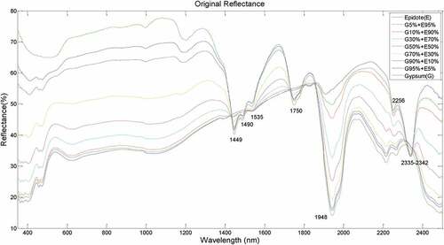
As a typical sulfate mineral, the reflectance spectrum of gypsum (CaSO4.2H2O) has three consecutive water absorption features at 1449 nm, 1490 nm, and 1535 nm, a diagnostic sulfate absorption feature at 1750 nm, and a strong water absorption feature at 1948 nm (shown in Figure 1). Epidote is a form of calcium silicate with the formula of Ca2Fe3+ Al2O.OH.Si2O7.SiO4. The spectrum of epidote has an absorption feature of Fe-OH at 2256 nm, and a diagnostic strong absorption feature between 2335 nm and 2342 nm. The intensity of the mixing spectra represented the mixture of gypsum and epidote, with a combination of the spectral features of both materials.

Figure 1. The spectra of laboratory mineral powders (2-endmember mixtures)

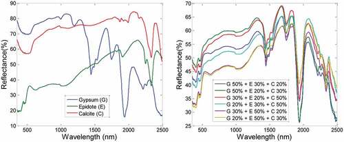
To make further research on more complicated situations, we also perform experiments on powder mixtures of three endmembers: gypsum, epidote, and calcite. The mixture scheme is in Table 2. The measuring conditions are the same as that of two-endmember mixtures. The spectra of endmembers and mixtures are shown in Figure 2.

Table 2. The compositions of laboratory mineral powders (3-endmember mixtures)

Mixture No.	Gypsum	Epidote	Calcite
Mixture 1	50%	30%	20%
Mixture 2	50%	20%	30%
Mixture 3	30%	20%	50%
Mixture 4	20%	30%	50%
Mixture 5	30%	50%	20%
Mixture 6	20%	50%	30%

Figure 2. The spectra of laboratory mineral powders (3-endmember mixtures). (left: endmembers; right: mixtures)

Airborne data

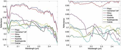
The Airborne Visible/Infrared Imaging Spectrometer (AVIRIS), operated by the NASA/Jet Propulsion Laboratory (JPL), is a 224-channel imaging spectrometer with approximately 10-nm spectral resolution that covers the 0.4–2.5 μm spectral range (Kruse, Boardman, & Huntington, 2003). The scene that was used for our experiment was the well-known image of the Cuprite mining district (NV, USA) captured by AVIRIS in 1997. Cuprite has been used as a geological remote sensing test site since the early 1980s, and many studies have been published (e.g. Goetz, Vane, & Solomon, 1985; Kruse, Boardman, & Huntington, 2002). The data used here were the reflectance dataset after correction using the Atmospheric REMoval (ATREM) (Gao & Goetz, 1990) and Empirical Flat Field Optimal Reflectance Transformation (EFFORT) (Boardman & Huntington, 1996) programs (1.96–2.51 μm, 50 bands). The endmember spectra (shown in Figure 3) were extracted using the pixel purity index (PPI) algorithm (Boardman, 1995). The reflectance data and endmember spectra were downloaded from the Exelis website (http://www.exelisvis.com, 11:00AM, 09/02/2015).

Figure 3. The endmember spectra of AVIRIS Cuprite data

To analyze the effects of atmospheric correction and verify the analysis results based on the above dataset, the reflectance datasets of the same scene after correction with ATREM and Flat Field (both without EFFORT processing) are introduced for comparison. These datasets were also downloaded from the Exelis website (http://www.exelisvis.com, 15:00AM, 01/02/2016). Lacking recognized endmembers for these two datasets, we select the pixels verified to be relatively pure as the endmembers. Usually, endmember should be the average spectrum of multi-pixels within the region of interest. However, only one single pure pixel in the image is available for each endmember, so selecting a single pixel as endmember is the easiest and most effective choice for this research. The accuracy of spectral unmixing can be decided by two factors: endmember extraction and spectral unmixing model. In order to investigate the effects of atmospheric correction on spectral unmixing models, we have to make sure that ATREM and Flat Field datasets have no difference in the endmember extraction process. Although atmospheric correction has strong influence on most endmember extraction methods, but it would not affect the relative relationship between the reconstruction accuracies of these two datasets, which can be used to analyze the robustness of these spectral unmixing models. The endmember spectra of these two datasets are shown in Figure 4. The coordinates and mineral components of these pixels in the image are listed in Table 3.

Table 3. Selected pixels for endmembers of ATREM and Flat Field datasets

Mineral Component	Sample	Line
Playa	590	570
Varnished Tuff	435	555
Silica	494	514
Alunite	531	541
Kaolinite	502	589
Buddingtonite	448	505
Calcite	260	613

Figure 4. The endmember spectra of ATREM and Flat Field datasets (left: ATREM; right: Flat Field)

Comparing the endmember spectra in Figure 4, it is obvious that atmospheric correction has significant influence on the waveform of reflectance spectra. In Flat Field dataset, some pixels have reflectance value more than 1. In the Flat Field method, the average spectrum of a highly reflective and a flat region was chosen as the reference spectrum, which might not be the maximum reflectance in the image. Consequently, some highly reflective pixels might have a reflectance value greater than one. Natural log result of real number above 1 will be positive number, and the result of number between 0 and 1 is negative. The endmember spectra must be all positive or all negative, so we have corrected the invalid values above 1 in Flat Field dataset to be 1. The ATREM dataset does not have this kind of problem.

Spectral unmixing models

Linear model

In the LMM, the reflectance of a pixel in each spectral band is expressed as a linear combination of the characteristic spectra of its component endmembers, weighted by their respective areal proportions within the pixel. Thus, the reflectance of a mixing pixel is given by (Bioucas-Dias, Plaza, & Dobigeon, 2012):

(1) $R=\sum _{i=1}^n{R}_i{a}_i+\epsilon ,$(1)

with i = 1,2,3…n, where $R_i$ denotes the reflectance of the ith component, $a_i$ is the abundance of the ith component in the pixel, n is the number of components in the pixel, and $\epsilon$is the error term.

If all the endmembers are included, the following additivity constraint will be satisfied:

(2) $\sum _{i=1}^n{a}_i=1.$(2)

Moreover, $a_i$ should meet the positivity conditions:

(3) $a_i\ge 0.$(3)

The algorithm for abundance estimation based on Formula 1 to 3 is called fully constrained least square (FCLS). Given the endmember spectra and the mixed spectra, we could determine the abundance of endmembers using FCLS.

Continuum removal model

Usually, the continuum is a convex hull fitted over the top of the spectrum. It consists of line segments connecting local maxima of the reflectance spectrum. The CR spectrum is realized using the following formula (Van der Meer, 2000):

(4) $R_{cr}=\frac{R}{R_c},$(4)

where $R_{cr}$is the spectrum for which the continuum is removed, $R$is the reflectance spectra, and $R_c$ is the spectra continuum. Through CR, the pure absorption features caused by transmitted radiation could be extracted. Here, we defined the linear spectral unmixing conducted on $R_{cr}$ as the CR model.

Natural log model

According to Beer–Lambert, the absorbance is directly proportional to the concentration of absorbers and the path length of irradiating energy. Therefore, to linearize the reflectance spectrum, natural log operation is often applied before quantitative analysis:

(5) $A=log(1/R),$(5)

where $A$ is the absorbance spectrum and $R$ is the reflectance spectrum. Absorbance is only rigorously defined for transmission through a non-scattering sample as $log(1/T)$, where $T$ is the transmittance spectrum. However, for reflectance spectra, the detected energy is composed of transmitted energy and non-transmitted energy (reflected energy). Through natural log operation, the transmitted energy can be linearized, but the non-transmitted energy is not effectively eliminated. Although lacking a functional relationship, NL model provides satisfactory results in usual applications of NIR diffuse reflectance spectroscopy (Blanco, Coello, & Iturriaga, 1998; Smith, Ollinger, & Martin, 2002). We defined the spectral unmixing model based on the absorbance spectrum as the NL model.

Log and continuum removal model

As stated in 2.2.3, the observed reflectance energy can be divided into the transmitted part and the non-transmitted part. For the non-transmitted part, the contributions of different endmembers are combined linearly. While for the transmitted part, natural log operation is needed for linearization. If we could separate these two parts, then a proper spectral unmixing model can be chosen easily. CR can be utilized to extract the transmitted energy. Accordingly, through combining the NL model and the CR model, alog and CR (LCR) model can be given.

In the LCR model, natural log operation was first performed on the reflectance spectra, and then the continuum was removed. For absorbance spectra, the continuum should be removed by subtraction, not division (Clark & Roush, 1984). Finally, linear spectral unmixing was performed on the pre-processed spectra. In some spectral deconvolution methods, such as modified Gaussian modeling (MGM), the data processing workflow is similar to the LCR model (Sunshine, Pieters, & Pratt, 1990). However, this is the first time that the LCR model has been proposed as a spectral unmixing model.

Simplified Hapke model

The Hapke model (Hapke, 1981) is the most widely used radiative transfer model. According to this model, the spectra of minerals and rocks are composed of two parts: a single scattering parameter, such as single scattering albedo (SSA) and scattering phase function; and a part related to multiple scattering behavior.

According to the Hapke model, bidirectional reflectance is given by:

(6) $R(i,e,g)=\frac{w}{4\pi }\frac{{\mu }_0}{{\mu }_0+\mu }[p(g)(1+B(g))+H(w,\mu )H(w,{\mu }_0)-1],$(6)

where $i$ is the angle of incidence, $e$ is the angle of emergence of detection, $g$ is the phase angle, $w$is the average single scattering albedo, $B(g)$ is the backscattering function, $p(g)$ is the average phase function of particles, and $H(w,\mu )$ is the multiple-scattering function: ${\mu }_0=cos(i)$, $\mu =cos(e)$.

B(g) can be only retrieved with datasets of different viewing geometries, which is not realistic in every real scene. When the scattering angle is larger than 15°, the $B(g)$ can be neglected (Mustard & Pieters, 1987). In the laboratory experiment, the scattering angle was 20°, which meets this condition. For the Cuprite data, according to the function of solar zenith angle, the solar altitude is approximately 75.8°, so the scattering angle is 14.2° (Bodhaine, Dutton, & Mckenzie, 1998). Although this is smaller than 15°, for the convenience of calculation, we chose to neglect the$B(g)$, and approximated the scattering angle at 15°. Assuming that scattering of a single mineral particle is isotropic (i.e. $p(g)=1$), function (6) can be simplified and transformed to obtain a single scattering albedo from the bidirectional reflectance data.

Accuracy analysis methods

Unmixing accuracy analysis

For laboratory samples, real fractions are available, so it is easy to calculate the unmixing accuracy using RMSE value. However, for image data, it is difficult to determine the real composition of each pixel, so it is hard to achieve a direct unmixing accuracy assessment. For a specific component in the mixture, the abundance RMSE (ARMSE) was used for estimation as follows:

(7) $ARMSE=\sqrt{\frac{\sum _{i=1}^m{(a_i-{a^{\prime }}_i)}^2}{m}},$(7)

where $a_i$ is the real abundance of each mixture, $a_i^{\prime }$is the calculated abundance of each mixture, and $m$ is the number of mixtures.

The following sections will introduce an evaluation system based on mixing reflectance spectra reconstruction.

Mixing reflectance reconstruction

After solving the fractions of endmembers, we were able to reconstruct the reflectance based on the above models to simulate the original reflectance data. By comparing the difference between the simulated reflectance data and original reflectance data, the effects of each model on spectral unmixing could be evaluated.

For the linear model, mixing reflectance could be directly simulated based on formula (1). For the other four models, inverse pre-processing was required to convert the mixing spectra back to reflectance spectra. Figure 5 presents a flow chart of the procedure for mixing reflectance reconstruction (MRR) data processing.

Figure 5. The flowchart of the data processing used in mixing reflectance reconstruction

Mixing reflectance reconstruction accuracy analysis

The accuracy of MRR could be evaluated individually from the spectral and spatial dimensions. Based on the spectral dimension, for each band a normalized RMSE value could be achieved, and their average value, maximum value, minimum value, and standard deviation could be used to describe the accuracy of a particular model. Based on the spatial dimension, for each pixel a normalized RMSE value could be determined, and the same four parameters could be calculated and compared between different models. Reconstruction RMSE (RRMSE) was used to estimate the reconstruction error as follows:

(8) $RRMSE=\frac{\sqrt{\sum _{i=1}^n{(y_i-y_i\prime )}^2/n}}{y_{max}-y_{min}},$(8)

where $y_i$ is real reflectance value at each sample, ${y_i}^{\prime }$ is the reconstructed reflectance value at each sample, n is the number of samples, $y_{max}$ is the maximum value of all samples, and $y_{min}$ is the minimum value of all samples.

However, if we combined the spectral and spatial dimensions, and transformed the three-dimensional reflectance data cube into a column vector, then a RRMSE value could be calculated for each model, which was called MRR accuracy analysis in the combined dimension in this paper. This process allowed effective comparison of the accuracy of different spectral unmixing models.

Data processing workflow

Workflow of laboratory data processing

To determine the effects of the NL and CR models, we set a total of five pre-processing conditions for the original reflectance data: NL, CR, NL plus CR, SH, and no processing at all (linear model). The processed data were then input into a FCLS processing, through which we could obtain the abundance estimation. Based on the estimated abundance and real abundance, an unmixing accuracy evaluation was conducted and the mixing reconstruction error was also calculated. Finally, based on the above results, the effects of the pre-processing methods and error evaluation indexes were comprehensively assessed. In particular, it is difficult to describe the spatial dimension for spectra collected by a pixel-based spectrometer. However, by assuming that the seven mixtures originated from different locations, each mixing spectrum could represent a pixel in the whole scene. From this perspective, we could conduct an MRR accuracy analysis in the spatial dimension. Figure 6 presents a flow chart of the analysis of laboratory data.

Figure 6. The flow chart of the analysis of laboratory data

Work flow of airborne data

The flow chart for the analysis of AVIRIS data was very similar to that for laboratory data, with the only differences being the unmixing algorithm and unmixing accuracy estimation (shown in Figure 7). We applied the Multiple Endmember Spectral Mixture Analysis (MESMA) algorithm via the Visualization and Image Processing for Environmental Research (VIPER) tool v1.5 (http://www.vipertools.org, 10:43AM, 09/17/2012), and selected the endmember composition group with least reconstruction error as the final result for each pixel. Both normalization and non-negative constraints were added, so the work flow was in accordance with that of laboratory data. For real image data, we could not obtain the real endmembers and their abundances, so estimation of the unmixing accuracy was not possible; therefore, only MRR accuracy estimation was performed.

Figure 7. Flow chart of the analysis of airborne data

Results

Results for laboratory data

Unmixing accuracy estimation

After performing FCLS on binary mixtures, the sum of abundance was one, and gypsum and epidote shared the same RMSE. Therefore, only the results for gypsum are listed (shown in Table 4). For the linear model, the estimated abundances were far less than the actual values, and the largest RMSE (0.1143) was recorded. If the ARMSE of the SH model (0.0262) was set as the standard, then the NL model was larger than the standard (0.0615), while the CR and LCR models were both smaller than the standard (0.017 and 0.0188). The NL model produced much better results than the linear model, but the RMSE was still larger than 5%. Generally, the estimated abundances of the CR model were slightly larger than those given by the LCR model, except when the abundance of gypsum is below 10%. They were both very accurate, with RMSE values were less than 1.9%.

Table 4. Abundance estimation results (volume proportion of gypsum) of the models (2-endmember (Gypsum (G) and Epidote (E)) powder mixtures)

Model	G5%+E95%	G10%+E90%	G30%+E70%	G50%+E50%	G70%+E30%	G90%+E10%	G95%+E5%	ARMSE
Linear	0.0332	0.0673	0.1963	0.3367	0.5297	0.7766	0.858	0.1143
NL	0.0409	0.0818	0.2419	0.4124	0.6198	0.8289	0.8908	0.0615
CR	0.0485	0.1061	0.3218	0.5193	0.7329	0.8954	0.9445	0.017
LCR	0.0533	0.1132	0.3209	0.5139	0.7179	0.875	0.9233	0.0188
SH	0.0446	0.0881	0.27	0.4685	0.6198	0.8652	0.9116	0.0262

Mixing reflectance reconstruction accuracy evaluation

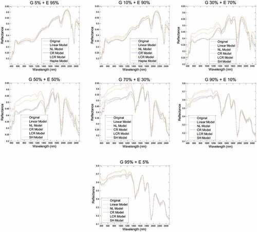
The MRR results of laboratory mixing spectra are shown in Figure 8. The LCR, CR, and SH models generally achieved very good results, while the NL model and the linear model performed relatively poorly. The LCR and CR models produced similar reconstruction results, and when epidote was dominant in the mixture, the MRR results were better. For the SH model, there was positive correlation between the proportion of gypsum in the mixture and the reconstruction accuracy.

Figure 8. Reconstructed spectra and real spectra of 2-endmember powder mixtures

Accuracy analysis in the spectral dimension

MRR error could be calculated in the spectral dimension for each sample; Figure 9 presents the results for the five models. The MRR error curves of all five models were similar, with several sharp peaks around 1500 nm, 1800 nm, and 2350 nm. These peaks correspond to the strong absorption features of the endmember minerals. Gypsum has three consecutive water absorption features around 1500 nm and a strong absorption feature around 1800 nm, while epidote has a diagnostic absorption feature around 2350 nm.

Figure 9. MRR error (RRMSE) of the models in the spectral dimension (2-endmember powder mixtures)

The boxplot of MRR error in the spectral dimension is presented in Figure 10. The boxplots in this paper were produced using OriginPro 8 software. If the input data is a matrix, there is one box per column. For the MRR error matrix, each model occupies a column, so there is one box for each model. On each box, the central mark is the median, the edges of the box are the 25th and 75th percentiles, the whiskers extend to the most extreme data points not considered outliers, and outliers are plotted individually. The results of the five models were similar, although the LCR model was the most accurate and the linear model was slightly weaker than the other models.

Figure 10. Boxplot of the MRR error (RRMSE) of the models in the spectral dimension (2-endmember powder mixture)

Accuracy analysis in the spatial dimension

The MRR error results of the seven mixing spectra were listed in Table 5. The LCR and SH models were generally more accurate. The LCR model had the smallest average RRMSE value, while the SH model had a very small standard deviation. For the SH model, the RRMSE values of the seven mixtures were very similar; for the other four models, when one component had a dominant role in the mixture, the reconstruction error was smaller. This finding suggests that the MRR accuracy of the SH model was not sensitive to the fractions of endmembers, whereas the other models were. To clarify these results, Figure 11 presents a boxplot of MRR results in the spatial dimension.

Table 5. MRR error (RRMSE) of the models in the spatial dimension (2-endmember (Gypsum (G) and Epidote (E)) powder mixtures)

	Linear	NL	CR	LCR	SH
G5%+E95%	0.027908	0.015606	0.015756	0.012116	0.036987
G10%+E90%	0.052744	0.02617	0.030343	0.020677	0.042839
G30%+E70%	0.166175	0.08781	0.063092	0.047876	0.049912
G50%+E50%	0.222277	0.131475	0.064524	0.052253	0.038602
G70%+E30%	0.16909	0.107397	0.054444	0.046206	0.029258
G90%+E10%	0.087845	0.066398	0.043102	0.039763	0.043497
G95%+E5%	0.059273	0.048862	0.030377	0.028746	0.037712
Mean	0.1122	0.0691	0.0431	0.0354	0.0398
Std	0.0734	0.0425	0.0185	0.0152	0.0065

Figure 11. Boxplot of MRR Error (RRMSE) in the spatial dimension (2-endmember powder mixtures)

Accuracy analysis in the combined dimension

To analyze the relationship between reconstruction error and abundance estimation accuracy, we also calculated the RRMSE of the results for the five models, and compared the sequence order of spectral unmixing accuracy and the reconstruction error (see Table 6).

Table 6. MRR error (RRMSE) of the models in the combined dimension (2-endmember powder mixtures)

Model	MRR Error (RRMSE)	Rank
Linear	0.0899	5
NL	0.0567	4
CR	0.0334	3
LCR	0.0282	1
SH	0.0311	2

Although the CR model achieved better spectral unmixing results than the SH model, it only achieved the third smallest RRMSE (0.0334) in the MRR results (shown in Table 6), which was larger than that of the SH model (0.0311). In general, the sequence of unmixing accuracy and the sequence of MRR accuracy were similar to each other, except for the CR model. Therefore, MRR error could be a qualified indicator of the performance of spectral unmixing in most situations when the actual proportions are not available. This approach was then applied to the analysis of AVIRIS data, as discussed in 3.1.3.

Multi-endmember mixture analysis

To analysis the accuracy of these spectral unmixing models for more complicated mixtures, powder mixtures of three endmemebers: gypsum, epidote, and calcite are processed in the same workflow in Figure 6. As the aim is to make comparison between these spectral unmixing models, only the results of reconstruction error are displayed in Table 7.

Table 7. MRR error (RRMSE) of the models in the combined dimension (3-endmember powder mixtures)

Model	MRR Error (RRMSE)	Rank
Linear	0.1940	5
NL	0.1269	4
CR	0.0615	3
LCR	0.0517	1
SH	0.0552	2

The RRMSE values of the three-endmember powder mixtures are larger than that of two-endmember mixtures, especially for the linear model and the NL model. This indicates that the spectral mixing mechanism can be more complicated for mixtures of three or more endmembers, and the linear model and the NL model are not very suitable for this kind of situation. However, the ranking sequence of three-endmember mixtures is exactly the same as that of two-endmember mixtures. It strongly verifies the effectiveness of previous experiments and model comparison results in 3.1.2. As for ARMSE results, the general model ranking sequence for ARMSE in the experiments on ternary mixtures was the same as that of binary mixtures.

The general model ranking sequence in the experiments on ternary mixtures was the same as that of binary mixtures (Table 7). For ternary mixtures, each component has a different ARMSE, so the results are much more complicated than binary mixtures, which will not be fully displayed in detail in this paper.

Results for airborne data

Unmixing results

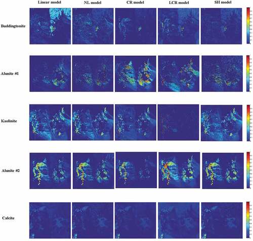
The unmixing results for the five models are shown in Figure 12. The abundance maps of the LCR model had more contrast, and the high abundance pixels were easy to identify because they were surrounded by low abundance pixels. The CR model also yielded good visibility. The NL and SH models produced very similar results.

Figure 12. Abundance maps of selected materials for the AVIRIS data. (top to bottom: buddingtonite, alunite #1, kaolinite, alunite#2, and calcite; left to right: linear model, NL model, CR model, LCR model, and SH model)

Mixing reflectance reconstruction accuracy analysis

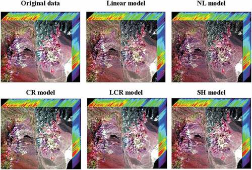
The MRR results for the five models together with the original reflectance data are shown in Figure 13. The MRR results were generally similar to the original reflectance data, and the quality differences were not obvious from the 3D data cubes. In the following sections, we evaluate the MRR results from spectral, spatial, and combined dimensions.

Figure 13. 3D data cubes of original reflectance data and MRR results. (line 1 from left to right: original data, linear model, NL model; line 2 from left to right: CR model, LCR model, and SH model)

Accuracy analysis in the spectral dimension

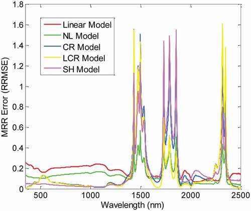
The RRMSE curves of the five models in the spectral dimension are shown in Figure 14. The error difference is apparent. The curve of the NL model is situated above the others, which indicates that it was the least accurate. The curves of the linear and SH model lie underneath and are close to each other. The LCR and CR models achieved the best accuracy, and at most bands, the LCR model was slightly more accurate than the CR model.

Figure 14. MRR error (RRMSE) of AVIRIS data in the spectral dimension

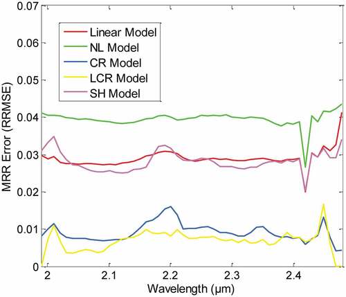
Some sharp peaks and valleys appeared on the RRMSE curves. Peaks were located around 2.01–2.02 μm, 2.2 μm, and 2.45 μm, while the valley of the linear model, NL model, and SH models was located at 2.42 μm. None of the above peaks or valleys was shared by all five models. For image data, the models had different changing trends in the spectral dimension, which was not the case for the laboratory data. This finding indicates that the formation of the peaks and valleys was not only related to the absorption features of the endmembers, but also the models themselves. Because the endmembers in this image were so complex, it is difficult to determine the exact causes of the valleys and peaks. This issue was beyond the scope of the present study, but future experiments involving other images or simulation data may help clarify the reasons for the peaks and valleys.

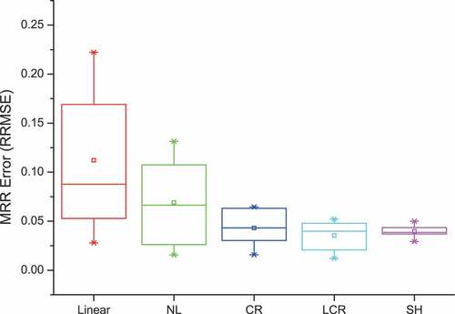
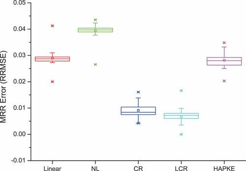
To better illustrate accuracy, Figure 15 presents a boxplot. As stated above, the LCR model had the best accuracy, while the NL model performed worst. In the spectral dimension, standard deviation values did not vary greatly between the five models.

Figure 15. Boxplot of the MRR error (RRMSE) of AVIRIS data in the spectral dimension

Accuracy analysis in the spatial dimension

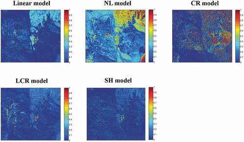
The MRR error in the spatial dimension is presented in Figure 16. The goal here is to show the characteristics of the error distribution for the different models, not the error value itself, so we set a different scale bar for each image to improve the visual effect.

Figure 16. Maps of MRR error (RRMSE) in the spatial dimension for AVIRIS Data

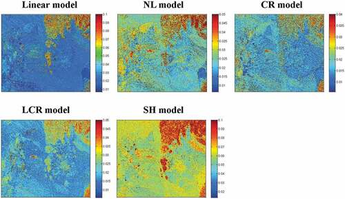
The error maps of different models had an obvious co-relationship with each other, and shared a common high error region at the center and top-right of the image. Considering the endmember effect, we selected the abundance map that was closest to the error maps from the individual unmixing results for each model; Figure 17 presents the results.

Figure 17. Abundance maps consistent with maps of MRR error (RRMSE)

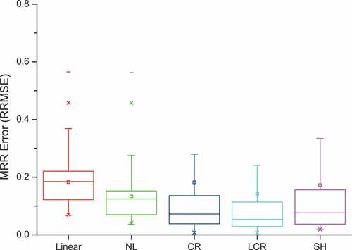
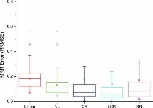
The boxplot of the spatial MRR error for the five models is presented in Figure 18. With the exception of the SH model, spatial MRR error was similar among the models. The LCR model and CR model outperformed the other models. The results for the linear model and the NL Model were very similar.

Figure 18. Boxplot of the MRR error (RRMSE) of AVIRIS data in the spatial dimension

Accuracy analysis in the combined dimension

The MRR error results for AVIRIS data in the combined dimension are listed in Table 8. The LCR and CR models had smaller RRMSE values than the other models, and LCR had the smallest RRMSE value (0.0050) in the list, which was also the case for mineral powder mixtures. The SH model and the linear model had RRMSE values of 0.0192 and 0.0196 separately, and the NL model had the largest RRMSE value (0.0269) in the list.

Table 8. MRR error for AVIRIS data in the combined dimension

Model	MRR Error (RRMSE)	Rank
Linear	0.0196	4
NL	0.0269	5
CR	0.0064	2
LCR	0.0050	1
SH	0.0192	3

With regard to the results of intimate mixtures, the linear model and the NL model still remained as the two most poorly performing models, and the linear model yielded better results than the NL model. This was largely because, at the spatial resolution of an aerial image, linear mixing plays a more important role in the whole spectral mixing process. Additionally, the physical properties of bare rock and mineral powder differ significantly. The NL model yielded poor results for both laboratory sample analysis and airborne image analysis, so it is doubtful that this model can be applied in practical applications.

Analysis of the atmospheric effects

To verify whether the model comparison results are the same for other datasets and investigate the influence of atmospheric correction on spectral unmixing models, the reflectance datasets after correction with ATREM and Flat Field were processed in the same workflow. Focusing on the accuracy comparison of different models and different datasets, only combined dimension MRR analysis is displayed here (shown in Table 9).

Table 9. MRR error (RRMSE) for ATREM and Flat Field datasets in the combined dimension

	ATREM		Flat Field
Model	RRMSE	Rank	RRMSE	Rank
Linear	0.0724	3	0.1725	4
NL	0.0953	4	0.1718	3
CR	0.0542	2	0.1366	2
LCR	0.0097	1	0.0224	1
SH	0.0981	5	0.3013	5

Generally, the RRMSE of the ATREM dataset is much smaller than that of the Flat Field dataset. Undoubtedly, ATREM has better correction accuracy than Flat Field method. This indicates that atmospheric correction has strong influence on spectral unmixing accuracy, and better atmospheric correction can improve the spectral unmixing accuracy. LCR model and CR model still outperformed the other models, and LCR model had much smaller RRMSE than the other models.

Discussions

In this study, the newly proposed log and CR (LCR) model and four other spectral unmixing models for mineral analysis (the linear model, CR model, natural log model, and simplified Hapke model) were summarized and applied to both laboratory mineral powder spectra and hyperspectral data. MRR was utilized to determine the unmixing accuracy, which was applied to different dimensions, such as spatial dimension and spectral dimension.

For laboratory data, the abundance estimation accuracy of different models was extracted and compared with the MRR results (Tables 4 and 6). For the linear model, the ARMSE value was larger than 10%. Previous experiments showed similar accuracy (Yan, Liu, & Wang, 2008). This finding strongly suggests that the linear model is not suitable for mineral powder mixtures. The accuracy of SH model is better than 5%, which is in accordance with previous research (Mustard & Pieters, 1987). The LCR model and the CR model had the highest accuracy. The good performance of the LCR model in both MRR and abundance estimation demonstrated its great potential for spectral mixture analysis. The fraction estimation results indicate that the absorption features have remarkable effects on the accuracy of spectral unmixing models, which was also proved in another study (Zhang et al., 2013).

In the spectral dimension, the MRR accuracy at different wavelengths was different, but all five models shared similar changing trends for the accuracy curves (Figure 9). In general, when a specific component was dominant in the mixture, the MRR accuracy was better, and the shortwave infrared bands had better MRR accuracy than the visible and near-infrared bands. The results of previous experiments were also in accordance with our conclusions (Yan et al., 2008). This phenomenon indirectly verifies the advantage of the shortwave infrared bands over NIR bands in mineral spectra analysis. The MRR accuracy near diagnostic absorption features was worse than that of the other wavelengths. This indicates that the spectral mixing mechanism is more complex within the band range of absorption features, which leads to relatively poor reconstruction accuracy. This is also supported by previous research (Zhao et al., 2013).

The scene for imagery analysis has been widely used in hyperspectral remote sensing and geologic research. In general, the abundance maps of the different models (Figure 12) were consistent and in accordance with previous mapping results (Kruse et al., 1990). When compared with the results for laboratory powder mixtures, the models with the smallest RRMSE in the combined dimension (Tables 7 and 8) did not change (i.e. LCR, CR, and SH models). This finding reveals that the LCR model improves mineral spectral unmixing, for intimate mixtures or aerial images, and provided accuracy even better than traditional radiative transfer models (such as the SH model). Additionally, it does not require a prior knowledge or any measurement parameters and is easy to perform. However, as mentioned in Section 2.2.5, B(g) was neglected in the SH model even though this simplification was not valid in the strict sense, which might be a reason for the relatively poor performance of SH model in the imagery analysis.

The distribution of the MRR accuracy in the spatial dimension showed close relationship with the distribution of specific endmembers, depending on the choice of spectral unmixing models. The types of endmember selected differed for each model (Figure 12), but were either buddingtonite or dark/black. This finding indicates that the spectra for these endmembers may not be representative, or that some endmembers were not located within the highly accurate region. The MRR error of the CR model was uniform for the whole image, which implies that in this model the MRR accuracy was only weakly influenced by spatial effects. This finding verifies that continuum-removal could eliminate the effects of topography, atmosphere, and illumination (Van der Meer, 2000).

In previous experiments, the LCR model and the CR model seem competitive. While in the experiment for analysis of effects of different atmospheric correction algorithms, the LCR model significantly outperformed the CR model in terms of MRR errors (Table 9). The ATREM model was proved to be superior to the Flat Field model in airborne image analysis (Huang et al., 2004). This result indicates that both the LCR model and the CR model work well but the LCR model has more robustness against atmospheric correction. In contrast, the SH model had the largest RRMSE value in this experiment. This implies that the SH model is very sensitive to the accuracy of atmospheric correction.

Conclusions

The choice of spectral unmixing model is essential for mineral abundance mapping using spectral analysis, but there is a lack of systematic research on how to make the choice. Continuum removal and natural log operation both have great potential in quantitative analysis of minerals, and the combination of them can be a strong contender for spectral unmixing. Therefore, we newly proposed the log and CR (LCR) model for spectral unmixing, conducted experiments on laboratory mineral mixtures and airborne hyperspectral data for bare rocks, and attempted to develop a comprehensive accuracy evaluation system for spectral unmixing. Five key findings were obtained:

1. A newly proposed LCR model is developed based on investigating the existing spectral unmixing algorithms and physical mechanism analysis. Existing models having typical applications related to mineral analysis, including the linear model, the natural-log (NL) model, the continuum-removal (CR) model and the simplified Hapke (SH) model, were also summarized.

2. Based on the concept of MRR, a thorough method to determine the accuracies of spectral unmixing models is proposed. The reconstruction error can be analyzed from the spectral dimension, the spatial dimension, and the combined dimension.

3. By measuring the spectra of proportionally mixed mineral powders, we were able to investigate and verify the relationship between MRR accuracy and spectral unmixing accuracy. This finding validates that when the actual fractions are not available, it is possible to estimate the spectral unmixing accuracy based on an MRR accuracy analysis.

4. Experiments on the well-known imagery data for Cuprite (NV, USA) allowed us to evaluate the effects of the five unmixing models based on an MRR accuracy analysis. The results revealed that the LCR model yielded good results in nearly all aspects and has considerable potential for practical application.

5. The effects of atmospheric correction on spectral unmixing accuracy were verified, but the level of influence was different for different unmixing models. The LCR model achieved the best results, which verified its robustness.

These findings provide a solid foundation for future research about spectral unmixing models. However, our experiments only included laboratory powder mixtures of specific minerals and airborne hyperspectral data. In future research, a wider range of intimate mixtures should be studied, including more types of minerals, core imaging spectrometer data, and hyperspectral data from the Moon or Mars. Based on this, a more comprehensive solution to mineral spectral mixture analysis can be developed. The accuracy evaluation method based on MRR may also be applied in other models, such as spectral unmixing models for urban areas, forests, and water bodies.

Acknowledgments

The author would like to thank Exelis Visual Information Solutions (which is now Harris Geospatial Solutions) for supplying the reflectance image data and endmember group.

Disclosure statement

No potential conflict of interest was reported by the authors.

Additional information

Funding

This work was supported by the Open Fund of State Key Laboratory of Remote Sensing Science [OFSLRSS201707]; National Natural Science Foundation of China [41701488]; Open Fund of State Key Laboratory of Coal Resources and Safe Mining (China University of Mining and Technology) [SKLCRSM16KFC02].

References

- Adams, J.B. (1974). Visible and near‐infrared diffuse reflectance spectra of pyroxenes as applied to remote sensing of solid objects in the solar system. Journal of Geophysical Research, 79(32), 4829–4836. doi:10.1029/JB079i032p04829
- Bioucas-Dias, J.M., Plaza, A., & Dobigeon, N. (2012). Hyperspectral unmixing overview: Geometrical, statistical, and sparse regression-based approaches. IEEE Journal of Selected Topics in Applied Earth Observations & Remote Sensing, 5(2), 354–379. doi:10.1109/JSTARS.2012.2194696
- Blanco, M., Coello, J., & Iturriaga, H. (1998). Near-infrared spectroscopy in the pharmaceutical industry. The Analyst, 123, 135R–150R. doi:10.1039/a802531b
- Boardman, J.W. (1995). Mapping target signatures via partial unmixing of AVIRIS data. Summaries of the Sixth Annual JPL Airborne Research Science Workshop, JPL Publication, 95(1), 23–26. Jet Propulsion Laboratory.
- Boardman, J.W., & Huntington, J.F. (1996). Mineral mapping with 1995 AVIRIS data. Summaries of the Sixth Annual JPL Airborne Research Science Workshop, JPL Publication, 96(1), 9–11. Jet Propulsion Laboratory.
- Bodhaine, B.A., Dutton, E.G., & Mckenzie, R.L. (1998). Calibrating broadband UV instruments: Ozone and solar Zenith angle dependence. Journal of Atmospheric & Oceanic Technology, 15(4), 916–926. doi:10.1175/1520-0426(1998)015<0916:CBUIOA>2.0.CO;2
- Brandmeier, M., Erasmi, S., & Hansen, C. (2013). Mapping patterns of mineral alteration in volcanic terrains using ASTER data and field spectrometry in Southern Peru. Journal of South American Earth Sciences, 48, 296–314. doi:10.1016/j.jsames.2013.09.011
- Chen, J., Richard, C., & Honeine, P. (2013). Nonlinear unmixing of hyperspectral data based on a linear-mixture/nonlinear-fluctuation model. IEEE Transactions on Signal Processing, 61(2), 480–492. doi:10.1109/TSP.2012.2222390
- Clark, R.N. (1999). Spectroscopy of rocks and minerals, and principles of spectroscopy. Manual of Remote Sensing, 3, 3–58.
- Clark, R.N., & Roush, T.L. (1984). Reflectance spectroscopy: Quantitative analysis techniques for remote sensing applications. Journal of Geophysical Research, 89(B7), 6329–6340. doi:10.1029/JB089iB07p06329
- Clark, R.N., Swayze, G.A., & Livo, K.E. (2003). Imaging spectroscopy: Earth and planetary remote sensing with the USGS Tetracorder and expert systems. Journal of Geophysical Research, 108(E12), 5131. doi:10.1029/2002JE001847
- Dobigeon, N., Tourneret, J., & Richard, C. (2013). Nonlinear unmixing of hyperspectral images: Models and algorithms. IEEE Signal Processing Magazine. doi:10.1109/MSP.2013.2279274
- Gao, B.C., & Goetz, A.F. (1990). Column atmospheric water vapor and vegetation liquid water retrievals from airborne imaging spectrometer data. Journal of Geophysical Research: Atmospheres (1984–2012), 95(D4), 3549–3564. doi:10.1029/JD095iD04p03549
- Goetz, A.F., Vane, G., & Solomon, J.E. (1985). Imaging spectrometry for earth remote sensing. Science, 228(4704), 1147–1153. doi:10.1126/science.228.4704.1147
- Halimi, A., Altmann, Y., & Dobigeon, N. (2011). Nonlinear unmixing of hyperspectral images using a generalized bilinear model. IEEE Transactions on Geoscience and Remote Sensing, 49(11), 4153–4162. doi:10.1109/TGRS.2010.2098414
- Hapke, B. (1981). Bidirectional reflectance spectroscopy: 1. Theory. Journal of Geophysical Research, 86(B4), 3039–3054. doi:10.1029/JB086iB04p03039
- Haykin, S.S. (2009). Neural networks and learning machines. Upper Saddle River: Pearson Education.
- Heylen, R., & Gader, P. (2014). Nonlinear spectral unmixing with a linear mixture of intimate mixtures model. IEEE Geoscience and Remote Sensing Letters, 11(7), 1195–1199. doi:10.1109/LGRS.2013.2288921
- Huang, Z., Turner, B.J., Dury, S.J., Wallis, I.R., & Foley, W.J.J.R.S.o.E. (2004). Estimating foliage nitrogen concentration from HYMAP data using continuum removal analysis. 93(1–2), 18-29. doi:10.1016/j.rse.2004.06.008
- Hunt, G.R. (1977). Spectral signatures of particulate minerals in the visible and near infrared. Geophysics, 42(3), 501–513. doi:10.1190/1.1440721
- Ichoku, C., & Karnieli, A. (1996). A review of mixture modeling techniques for sub‐pixel land cover estimation. Remote Sensing Reviews, 13(3–4), 161–186. doi:10.1080/02757259609532303
- Kruse, F.A. (1988). Use of airborne imaging spectrometer data to map minerals associated with hydrothermally altered rocks in the northern Grapevine Mountains, Nevada, and California. Remote Sensing of Environment, 24(1), 31–51. doi:10.1016/0034-4257(88)90004-1
- Kruse, F.A., Kierein-Young, K.S.,Boardman, J.W. (1990). Mineral mapping at cuprite, nevada with a 63-channel imaging spectrometer. Photogrammetric Engineering and Remote Sensing, 56:83-92.
- Kruse, F.A., Boardman, J.W., & Huntington, J.F. (2002). Comparison of EO-1 Hyperion and airborne hyperspectral remote sensing data for geologic applications. 2002 IEEE on Aerospace Conference Proceedings (pp. 3–1501). IEEE. doi: 10.1109/AERO.2002.1035288
- Kruse, F.A., Boardman, J.W., & Huntington, J.F. (2003). Comparison of airborne hyperspectral data and EO-1 Hyperion for mineral mapping. IEEE Transactions on Geoscience and Remote Sensing, 41(6), 1388–1400. doi:10.1109/TGRS.2003.812908
- Li, C., Fang, F., & Zhou, A. (2014). A novel blind spectral unmixing method based on error analysis of linear mixture model. IEEE Geoscience and Remote Sensing Letters, 11(7), 1180–1184. doi:10.1109/LGRS.2013.2285926
- Lucey, P.G., Blewett, D.T., & Hawke, B.R. (1998). Mapping the FeO and TiO2 content of the lunar surface with multispectral imagery. Journal of Geophysical Research, 103(E2), 3679–3699. doi:10.1029/97JE03019
- Meer, F.D.V.D., Werff, H.M.A.V.D., & Ruitenbeek, F.J.A.V. (2012). Multi- and hyperspectral geologic remote sensing: A review. International Journal of Applied Earth Observation & Geoinformation, 14(1), 112–128. doi:10.1016/j.jag.2003.09.001
- Mustard, J.F., & Pieters, C.M. (1987). Quantitative abundance estimates from bidirectional reflectance measurements. Journal of Geophysical Research: Solid Earth (1978–2012), 92(B4), E617–E626. doi:10.1029/JB092iB04p0E617
- Nascimento, J.M.P., & Bioucas-Dias, J.M. (2010). Unmixing hyperspectral intimate mixtures. Proceeding of SPIE. doi:10.1117/12.865118
- Nascimento, J.M.P., & Dias, J.M.B. (2005). Does independent component analysis play a role in unmixing hyperspectral data? IEEE Transactions on Geoscience & Remote Sensing, 43(1), 175–187. doi:10.1109/TGRS.2004.839806
- Neville, R.A., Lévesque, J., & Staenz, K. (2003). Spectral unmixing of hyperspectral imagery for mineral exploration: Comparison of results from SFSI and AVIRIS. Canadian Journal of Remote Sensing, 29(1), 99–110. doi:10.5589/m02-085
- Pelkey, S.M., Mustard, J.F., & Murchie, S. (2007). CRISM multispectral summary products: Parameterizing mineral diversity on Mars from reflectance. Journal of Geophysical Research: Planets (1991–2012), 112(E8). doi:10.1029/2006JE002831
- Plaza, A., Martín, G., & Plaza, J. (2011). Recent developments in endmember extraction and spectral unmixing. Optical Remote Sensing, 235–267. doi:10.1007/978-3-642-14212-3_12
- Schmidt, F., Legendre, M., & Le Mouëlic, S. (2014). Minerals detection for hyperspectral images using adapted linear unmixing: LinMin. Icarus, 237, 61–74. doi:10.1016/j.icarus.2014.03.044
- Smith, M., Ollinger, S.V., & Martin, M.E. (2002). Direct estimation of aboveground forest productivity through hyperspectral remote sensing of canopy nitrogen. Ecological Applications, 12(5), 1286–1302. doi:10.2307/3099972
- Sunshine, J., Pieters, C., & Pratt, S. (1990). Deconvolution of mineral absorption bands- An improved approach. Journal of Geophysical Research, 95(B5), 6955–6966. doi:10.1029/JB095iB05p06955
- Sunshine, J.M., & Pieters, C.M. (1993). Estimating modal abundances from the spectra of natural and laboratory pyroxene mixtures using the modified Gaussian model. Journal of Geophysical Research, 98(E5), 9075–9087. doi:10.1029/93JE00677
- Teye, E., Huang, X., & Afoakwa, N. (2013). Review on the potential use of near infrared spectroscopy (NIRS) for the measurement of chemical residues in food. American Journal of Food Science and Technology, 1(1), 1–8. doi:10.12691/ajfst-1-1-1
- Van der Meer, F. (2000). Spectral curve shape matching with a continuum removed CCSM algorithm. International Journal of Remote Sensing, 21(16), 3179–3185. doi:10.1080/01431160050145063
- Van der Meer, F.D., van der Werff, H., & van Ruitenbeek, F.J. (2012). Multi-and hyperspectral geologic remote sensing: A review. International Journal of Applied Earth Observation and Geoinformation, 14(1), 112–128. doi:10.1016/j.jag.2011.08.002
- Yan, B., Liu, S., & Wang, R. (2008). Experiment study on quantitative retrieval of mineral abundances from reflectance spectra. Society of Photo-Optical Instrumentation Engineers (SPIE) Conference Series (Vol. 3). doi: 10.1117/12.815549
- Yan, B., Wang, R., & Gan, F. (2010). Minerals mapping of the lunar surface with Clementine UVVIS/NIR data based on spectra unmixing method and Hapke model. Icarus, 208(1), 11–19. doi:10.1016/j.icarus.2010.01.030
- Zhang, C., Kovacs, J.M., & Wachowiak, M.P. (2013). Relationship between Hyperspectral Measurements And Mangrove Leaf Nitrogen Concentrations. Remote Sensing, 5(2), 891–908. doi:10.3390/rs5020891
- Zhang, J., Rivard, B., & Sanchez-Azofeifa, A. (2004). Derivative spectral unmixing of hyperspectral data applied to mixtures of lichen and rock. IEEE Transactions on Geoscience and Remote Sensing, 42(9), 1934–1940. doi:10.1109/TGRS.2004.832239
- Zhao, H., Zhang, L., & Cen, Y. (2013). Research on the characteristics of strong linearly related bands based on derivative of ratio spectroscopy. Journal of Infrared and Millimeter Waves, 32(6), 563–568. doi:10.3724/SP.J.1010.2013.00563
- Zhao, H., Zhang, L., & Wu, T. (2013). Research on the model of spectral unmixing for minerals based on derivative of ratio spectroscopy. Spectroscopy and Spectral Analysis, 33(1), 172–176. doi:10.3964/j.issn.1000-0593(2013)01-0172-05