Evaluating observed versus predicted forest biomass: R-squared, index of agreement or maximal information coefficient?

ABSTRACT

The accurate prediction of forest above-ground biomass is nowadays key to implementing climate change mitigation policies, such as reducing emissions from deforestation and forest degradation. In this context, the coefficient of determination ($R^2$) is widely used as a means of evaluating the proportion of variance in the dependent variable explained by a model. However, the validity of $R^2$ for comparing observed versus predicted values has been challenged in the presence of bias, for instance in remote sensing predictions of forest biomass. We tested suitable alternatives, e.g. the index of agreement ($d$) and the maximal information coefficient ($MIC$). Our results show that $d$ renders systematically higher values than $R^2$, and may easily lead to regarding as reliable models which included an unrealistic amount of predictors. Results seemed better for $MIC$, although $MIC$ favoured local clustering of predictions, whether or not they corresponded to the observations. Moreover, $R^2$ was more sensitive to the use of cross-validation than $d$ or $MIC$, and more robust against overfitted models. Therefore, we discourage the use of statistical measures alternative to $R^2$ for evaluating model predictions versus observed values, at least in the context of assessing the reliability of modelled biomass predictions using remote sensing. For those who consider $d$ to be conceptually superior to $R^2$, we suggest using its square $d^2$, in order to be more analogous to $R^2$ and hence facilitate comparison across studies.

KEYWORDS:

• Model assessment
• overfitting
• biomass
• LIDAR

Introduction

Obtaining accurate predictions of forest above-ground biomass ($AGB$) is nowadays key to estimating total carbon stock and implementing climate change mitigation policies, such as reducing emissions from deforestation and forest degradation (REDD) (Agrawal, Nepstad, & Chhatre, 2011; Eggleston, Buendia, Miwa, Ngara, & Tanabe, 2006; UNFCCC, 2014). To facilitate REDD implementation, tree allometry models are currently being developed in order to avoid the need for destructive sampling (Basuki, van Laake, Skidmore, & Hussin, 2009; Chave et al., 2005, 2014; Cuny et al., 2015; Iais et al., 2011; Krainovic, Almeida, & Sampaio, 2017; Marshall et al., 2012; Sawadogo et al., 2010). Methods combining field measurements and remote sensing technologies can provide robust and cost-effective means for reliably predicting $AGB$ from large areas of forests (Asner, 2011; Clark & Kellner, 2012; Goetz & Dubayah, 2014). For this reason, earth observation technologies using remote sensors are also nowadays extensively used to obtain predictions over large areas (Adnan et al., 2019; Asner & Mascaro, 2014; Bottalico et al., 2017; Hansen et al., 2013; Næsset, 2004; Tyukavina et al., 2017). Methods developed for $AGB$ estimation made use of the predictive power of spectral sensors (e.g. Franco-Lopez, Ek, & Bauer, 2001), LIDAR (e.g. Coomes et al., 2017; d’Oliveira, Reutebuch, McGaughey, & Andersen, 2012; Domingo, Lamelas, Montealegre, García-Martín, & de la Riva, 2018; García, Riaño, Chuvieco, & Danson, 2010; Montealegre, Lamelas-Gracia, García-Martín, de la Riva-Fernández, & Escribano-Bernal, 2017) or combinations of both (e.g. Asner, 2009; Bright, Hicke, & Hudak, 2012; Egberth et al., 2017; Estornell, Ruiz, Velázquez-Martí, & Hermosilla, 2012; Hernando et al., 2019). Zolkos et al., (2013) compiled a comprehensive revision of studies obtaining remote sensing predictions of $AGB$ by calibrating regional models with field plot information.

The correct evaluation of $AGB$ models is key to REDD, as errors may propagate when $AGB$ estimations are upscaled (Chave et al., 2004; Molto, Rossi, & Blanc, 2013; Valbuena et al., 2016). However, there is at the moment a critical lack of consensus on good practices for predicting forest $AGB$, both in the determination of allometric biomass equations (Sileshi, 2014; Temesgen, Affleck, Poudel, Gray, & Sessions, 2015) and in the evaluation of $AGB$ predictions using remote sensing methods (Loew et al., 2017; Valbuena et al., 2017a). The large variety of modelling methods and approaches for evaluating their accuracy complicates meta-analyses comparing various approaches (Loew et al., 2017; Zolkos et al., 2013). In a recent article (Valbuena et al., 2017a), we focused on the evaluation of final $AGB$ predictions from remote sensing with measures of accuracy and precision. We recommended the use of Piñeiro, Perelman, Guerschman, and Paruelo (2008) hypothesis test, considered the usability of Theil’s (1958) partial inequality coefficients, and suggested means for preventing overfitting to the sample (Valbuena et al., 2017a). In this paper, we focus on the evaluation of agreement between the $AGB$ observed and the $AGB$ predicted by the model.

The agreement between the observed and predicted values is an important indicator in model evaluation, and the best approach for its assessment is a subject of current discussion (Duveiller, Fasbender, & Meroni, 2016; Loew et al., 2017; Simon & Tibshirani, 2011; Willmott, Robeson, & Matsuura, 2012). The coefficient of determination ($R^2$) is widely used as the most suitable statistic for describing the agreement of model predictions with those observed empirically. $R^2$ expresses the proportion of variance in the dependent variable explained by a model. However, the use of $R^2$ in performance evaluation for predictive methods has been criticized for not being necessarily related to the accuracy of predictions (e.g. Fox, 1981; Paruelo, Jobbágy, Sala, Lauenroth, & Burke, 1998; Willmott, 1982). Alternatives have been proposed, such as the index of agreement ($d$), which can be interpreted as the relative prediction error (Willmott, 1981; Willmott & Wicks, 1980). Ever since, it has been popular in a variety of fields such as hydrology (Legates & McCabe, 1999; López-Moreno, Latron, & Lehmann, 2010), agriculture (Nendel et al., 2013), neurology (Ganpule et al., 2017), meteorology (Aschonitis et al., 2017; Morsy, El-Sayed, & Ouda, 2016), forest ecology (Ibrom et al., 2007; Ward, Bell, Clark, & Ram, 2013), or climate change (Bring & Destouni, 2014; Gaitan, Hsieh, & Cannon, 2014; Oyler, Ballantyne, Jencso, Sweet, & Running, 2015). The use of Willmott’s $d$ in remote sensing literature has, however, been marginal (Almeida et al., 2016; García et al., 2010; Grzegozewski, Johann, Uribe-Opazo, Mercante, & Coutinho, 2016; Wachholz de Souza, Mercante, Johann, Camargo Lamparelli, & Uribe-Opazo, 2015; Yebra & Chuvieco, 2009). Since many of these authors recommended the use of $d$ above $R^2$, this research was devoted to study the convenience of using $d$ for reporting the agreement between remote sensing $AGB$ predictions and their observed values. In addition to $d$, we postulated that using the recently developed maximal information coefficient ($MIC$) (Reshef et al., 2011) as a means for evaluating observed versus predicted values may be advantageous. $MIC$ was conceived as a non-parametric alternative to correlation, in the context of evaluating relationships between explanatory and response variables (Speed, 2011). Despite being very recent, it has already been found useful in a wide variety of contexts, such as microbiology (Thomas, Bordron, Eveillard, & Michel, 2017), medicine (Vallières et al., 2017), big data analysis (Chen & Yang, 2016), and also remote sensing (Görgens, Valbuena, & Rodríguez, 2017). Although it has been suggested that the robustness of this statistic against noise should be studied in terms of measuring predictive accuracy of models (Loew et al., 2017; Murrell, Murrell, & Murrell, 2014), to our knowledge no previous study has considered the suitability of $MIC$ in the context of evaluating the agreement between modelled predictions of $AGB$ and their corresponding observed values.

In this article, we consider the adequacy of using alternatives to the $R^2$ for evaluating the agreement between observed and predicted values. The alternatives considered were $d$ and $MIC$, and the study was conceived as a further aspect of prediction accuracy to be revised in the context of $AGB$ predictions from remote sensing, additional to those outlined in Valbuena et al. (2017a). We, therefore, followed up the same experimental design to allow direct comparison and contrasting against additional measures of accuracy: results are presented for unviable modelling approaches alongside correct ones, in order to highlight whether the alternative measures of agreement reliably make a difference among them.

Material and methods

Field and remote sensing datasets

The study employed data from $n=37$ field plots composed of two concentric circles of radii 10 m and 20 m (Valbuena et al., 2013b), which were obtained in the summer 2006 at the Pinus sylvestris-dominated forests of Valsaín (Spain, approx. lat.: 41°04ʹ N, lon.: 4°09ʹ W; 1.3–1.5 km a.s.l.). Within the inner circle, all trees were measured, including seedlings and saplings, whereas the outer circle only were measured trees with diameter at breast height (dbh, cm) above 10 cm. Plot expansion factors were used to expand the forest information sampled within the inner plot to the outer plot (Valbuena, Packalen, Mehtätalo, Garcia-Abril, & Maltamo, 2013c). Treetop heights (h, m) were determined for every individual tree using a Vertex III Hypsometer (Haglof, Sweden). Plot centres were staked out using a HiPer-Pro (Topcon, California) receiver set at 1–2 m above the ground for differentially corrected global navigation satellite systems (GNSS) positioning (Valbuena, Mauro, Rodriguez-Solano, & Manzanera, 2012). Tree allometry (Montero, Ruiz-Peinado, & Muñoz, 2005) was used to calculate plot $AGB$ (Mg·ha⁻¹) from these field measurements. While Ruiz-Peinado, Del Rio, and Montero (2011) improved Montero et al.’s (2005) models by including a property of additivity among biomass components, we considered such property would not propagate to the remote sensing predictions with the methodology employed in this article (Hernando et al., 2019). The remote sensing survey was carried out in September 2006 using a LIDAR system (ALS50-II from Leica Geosystems, Switzerland) and a multispectral camera (DMC from Zeiss-Intergraph, Germany). The LIDAR pulse density was 1.15 pulses·m⁻², and approximate footprint diameter was 0.5 m at the ground. Using Terrascan (Terrasolid, Finland) returns were classified and those at the ground were interpolated into a digital terrain model (Valbuena, Mauro, Arjonilla, & Manzanera, 2011). DMC original multispectral bands had an approximate spatial resolution of 60 cm. The fusion of both remote sensors’ information was done with an assured perfect fit via a back-projection data fusion algorithm (Valbuena et al., 2013a, 2011). The correspondence between the field and remote sensing data was guaranteed with survey-grade and differentially corrected GPS positioning (Valbuena et al., 2012). Remote sensing predictors were computed from statistical descriptors of the distributions of heights from the LIDAR data, and normalised difference vegetation index (NDVI) values from the multispectral sensor (Manzanera et al., 2016). More details about the data employed and processing steps can be further scrutinized from Valbuena et al. (2017b), Appendix A, and the above-listed references. Readers interested in comparable studies in Mediterranean pine forest ecosystems in Spain may refer to a recent review in Gómez et al. (2019), or individual studies using LIDAR (Adnan et al., 2019; Bottalico et al., 2017; Estornell, Ruiz, Velázquez-Martí, & Hermosilla, 2011; García et al., 2010; Gonzalez-Ferreiro, Dieguez-Aranda, & Miranda, 2012; González-Olabarria, Rodríguez, Fernández-Landa, & Mola-Yudego, 2012; Montealegre, Lamelas, de la Riva, García-Martín, & Escribano, 2016; Montealegre et al., 2017; Valbuena et al., 2013c), in combination with multispectral sensors (Estornell et al., 2012; Hernando et al., 2019; Manzanera et al., 2016; Valbuena et al., 2013a, 2017b, 2011), or comparing methods for selection of predictor variables (Garcia-Gutierrez et al., 2014; Valbuena et al., 2017a) or prediction methods (García-Gutiérrez, Martínez-Álvarez, Troncoso, & Riquelme, 2015; Guerra-Hernández et al., 2016; Domingo, Lamelas-Gracia, Montealegre-Gracia, & de la Riva-Fernández, 2017; Domingo et al., 2018; Valbuena et al., 2016).

Modelling alternatives compared

The values of $R^2$, $d$ and $MIC$ calculated in this study were obtained for the same modelling alternatives reported in Valbuena et al. (2017a), in order to allow direct comparisons according to the conclusions reached in that study. These consisted in predictions of plot-level $AGB$ using parametric models and a non-parametric method: best-subset, step-wise and most similar neighbours, all of them including ‘restricted’ versions according to Piñeiro et al. (2008) and Valbuena et al. (2017a). All computations were carried out using the R statistical environment (version 3.3.1; R Development Core Team, 2016). The parametric models were power models adjusted in their linear form, i.e. using a natural logarithm transform of the response variable (e.g. Asner & Mascaro, 2014; Hudak et al., 2006; Næsset, 2002), which were bias-corrected when transformed back to the original scale (Baskerville, 1972; Sprugel, 1983). A first alternative, here forth denominated “best-subset” (Hudak et al., 2006; Miller, 1984), selected model predictors via exhaustive evaluation of all possible combinations using package “leaps” of R (Lumley & Miller, 2009), and minimization of Mallows’ Cp (Mallows, 1973) as predictor selection criteria. Next, there was a modification of this alternative here forth denominated “best-subset restricted overfitting” (Valbuena et al., 2017a). It consisted in further constraining the “best-subset” result by restricting the inflation of sum of squares to a 10% in the cross-validation, to avoid models overfitted to the sample (Ehrenberg, 1982; Lipovetsky, 2013; Weisberg, 1985), plus positive results in Piñeiro et al.’s (2008) hypothesis test to the observed versus predicted fit. The next alternative employed the same power model but variables were selected according to a step-wise procedure (Næsset, 2002; Weisberg, 1985) and the corrected Akaike Information Criterion (AIC) (Burnham & Anderson, 2002; Sugiura, 1978), as implemented in the function “stepAIC” of R (Venables & Ripley, 2002). We denominate this method “step-wise”, and also presented a “step-wise restricted overfitting” modification using the hypothesis test and the limiting criterion of 10% inflation in sums of squares (Valbuena et al., 2017a).

The other alternative employed was the non-parametric prediction. This was based on the most similar neighbour (MSN) method, one type of machine learning approach among the so-called group of nearest neighbour methods (Franco-Lopez et al., 2001; McInerney, Suárez, Valbuena, & Nieuwenhuis, 2010; McRoberts, Nelson, & Wendt, 2002). MSN predictions were carried out using the “yaImpute” package of R (Crookston & Finley, 2007). We set the algorithm to use inverse distance weighting averaging of three neighbours, based on previous experience (Almeida et al., 2016; Eskelson et al., 2009; Valbuena, Vauhkonen, Packalén, Pitkanen, & Maltamo, 2014). In the case of MSN, we employed canonical regression analysis (Cohen, Maiersperger, Gower, & Turner, 2003; Manzanera et al., 2016) to recursively select the predictors. The final selection criterion was the root mean squared error minimization with the same above-mentioned limiting restrictions of Piñeiro et al.’s (2008) hypothesis tests and avoiding overfitting (Valbuena et al., 2017a). Additionally, we calculated results also for a wide range of number of predictors $p=1\dots 30$, with the intention to emphasize whether the chosen statistics of agreement between observed and predicted would show any differences for unrealistically low $n/p$ ratios.

Evaluating the agreement between observed and predicted $AGB$

For all the modelling alternatives considered, we computed predictions using two options: first, (1) the model fit employing the entire dataset of $i=1\dots n$ forest plots used to train the model (i.e. model residuals without external validation), and also (2) a leave-one-out cross-validation removing each case $i$ from the training data as a prior step to the whole modelling process. In results, these two options are denoted using superscripts (or subscripts) $fit$ and $cv$, respectively. Thus, the training dataset used was the vector of measured $AGB$ values at plot-level $O=ob{s}_i$ where $ob{s}_i=ob{s}_1,\dots ,ob{s}_n$, from which we obtained the vector of modelled predictions $P=pr{e}_i$ where $pr{e}_i=pr{e}_1,\dots ,pr{e}_n$. These predictions where either those fitted in model training $\left(pr{e}_i^{fit}\right)$, or those calculated using cross-validation $\left(pr{e}_i^{cv}\right)$, since both were employed to compute the range of statistical measures considered for describing the agreement between observed and predicted. Therefore, $pr{e}_i$ denotes either $pr{e}_i^{fit}$ or $pr{e}_i^{cv}$ in the following equations detailing the measurements of agreement considered:

(1) The coefficient of determination, which shows the ratio of the sum of squared residuals to the total sum of squares:

(1) $\begin{array}{r}{R}^2=1-\left[{\sum }_{i=1}^n{\left(pr{e}_i-ob{s}_i\right)}^2/{\sum }_{i=1}^n{\left(ob{s}_i-\overline{obs}\right)}^2\right]\end{array}$(1)

(2) Willmott’s index of agreement, which was originally suggested to be (Willmott & Wicks, 1980):

(2) $\begin{array}{rl}& d=1-\left[{\sum }_{i=1}^n{\left(pr{e}_i-ob{s}_i\right)}^2\right./\\ & \left.{\sum }_{i=1}^n{\left(\left|pr{e}_i-\overline{obs}\right|+\left|ob{s}_i-\overline{obs}\right|\right)}^2\right]\end{array}$(2)

It was later suggested, however, that squaring the residuals may be an inconvenient approach (Willmott et al., 1985), and therefore they suggested the following refinement:

(3) $\begin{array}{rl}& d_1=1-\left[{\sum }_{i=1}^n\left|pr{e}_i-ob{s}_i\right|/\right.\\ & \left.{\sum }_{i=1}^n\left(\left|pr{e}_i-\overline{obs}\right|+\left|ob{s}_i-\overline{obs}\right|\right)\right]\end{array}$(3)

And also another further modification was suggested more recently (Willmott et al., 2012):

(4) $d_r=1-\left[{\sum }_{i=1}^n\left|pr{e}_i-ob{s}_i\right|/2{\sum }_{i=1}^n\left|ob{s}_i-\overline{obs}\right|\right]$(4)

The full version of the refined index of agreement $d_r$ consists of inverting the fraction and subtracting one from it (Willmott et al., 2012: Equation (5)(5) $\begin{array}{r}MI(P,O)=\sum _{P,O}p(P,O)\cdot log[p(P,O)/p(P)p(O)]\end{array}.$(5) ), in order to accommodate poorly performing models. However, this was not necessary in our case since the agreement between observed and predicted was higher for all the modelling alternatives considered.

(3) The maximal information coefficient, which measures the entropy of the relationship (Reshef et al., 2011; Speed, 2011). It is based on the naïve mutual information $MI\left(P,O\right)$ (Linfoot, 1957). The computation of $MIC$ involves binning $P$ and $O$, calculating relative abundances $p\left(P,O\right)$ at each grid of the resulting cell, and consider the overall uncertainty in their relationship using Shannon’s (1948) entropy:

(5) $\begin{array}{r}MI(P,O)=\sum _{P,O}p(P,O)\cdot log[p(P,O)/p(P)p(O)]\end{array}.$(5)

In Reshef et al.’s (2011) algorithm, $MIC$ results from the bin size that maximizes $MI\left(P,O\right)$:

(6) $MIC=\underset{P,O_{total}<B}{max}\left\{MI\left(P,O\right)/log\left[min\left(P,O\right)\right]\right\}$(6)

We employed the R implementation for $MIC$ computation available in package “minerva” (Filosi, Visintainer, & Albanese, 2014).

While the calculation of $d$ resembles that of a sample Pearson’s correlation coefficient ($r$), $MIC$ is customarily interpreted as a non-parametric version of a correlation coefficient (Görgens et al., 2017). Also, Simon and Tibshirani (2011) recommended the use of Brownian distance correlation (Székely & Rizzo, 2009) above $MIC$. For these reasons, we also calculated from our dataset the following statistics for additional discussion on the most convenient approach for assessing the agreement between observed versus predicted in model evaluation:

(4) The coefficient of correlation between observed and predicted values, calculated from Pearson’s product moment correlation:

(7) $\begin{array}{rl}& r=\left[{\sum }_{i=1}^n\left(pr{e}_i-\overline{pre}\right)\left(ob{s}_i-\overline{obs}\right)\right]/\\ & \left[\sqrt{{\sum }_{i=1}^n{\left(pr{e}_i-\overline{pre}\right)}^2}\sqrt{{\sum }_{i=1}^n{\left(ob{s}_i-\overline{obs}\right)}^2}\right]\end{array}$(7)

(5) The distance correlation ($dCor$) is an approach to evaluating the relationship between two variables based on their energy (Székely & Rizzo, 2017), i.e., in this case, the distances between $\left(P,O\right)$ data in the metric space. We employed the distance correlation statistic implemented in the package “energy” of R (Rizzo & Szekely, 2017).

All the alternatives for evaluating the degree of agreement between observed and predicted were calculated both from the model fit predictions $\left(P^{fit}\right)$ and the cross-validated versions $\left(P^{cv}\right)$: $R_{fit}^2$, $R_{cv}^2$ (Equation (1)(1) $\begin{array}{r}{R}^2=1-\left[{\sum }_{i=1}^n{\left(pr{e}_i-ob{s}_i\right)}^2/{\sum }_{i=1}^n{\left(ob{s}_i-\overline{obs}\right)}^2\right]\end{array}$(1) ), $d^{fit}$, $d^{cv}$ (Equation (2)(2) $\begin{array}{rl}& d=1-\left[{\sum }_{i=1}^n{\left(pr{e}_i-ob{s}_i\right)}^2\right./\\ & \left.{\sum }_{i=1}^n{\left(\left|pr{e}_i-\overline{obs}\right|+\left|ob{s}_i-\overline{obs}\right|\right)}^2\right]\end{array}$(2) ), and $MI{C}^{fit}$, $MI{C}^{cv}$ (Equation (5)(5) $\begin{array}{r}MI(P,O)=\sum _{P,O}p(P,O)\cdot log[p(P,O)/p(P)p(O)]\end{array}.$(5) ); plus the refined versions of Willmott’s agreement $d_1^{fit}$, $d_1^{cv}$ (Equation (3)(3) $\begin{array}{rl}& d_1=1-\left[{\sum }_{i=1}^n\left|pr{e}_i-ob{s}_i\right|/\right.\\ & \left.{\sum }_{i=1}^n\left(\left|pr{e}_i-\overline{obs}\right|+\left|ob{s}_i-\overline{obs}\right|\right)\right]\end{array}$(3) ), and $d_r^{fit}$, $d_r^{cv}$ (Equation (4)(4) $d_r=1-\left[{\sum }_{i=1}^n\left|pr{e}_i-ob{s}_i\right|/2{\sum }_{i=1}^n\left|ob{s}_i-\overline{obs}\right|\right]$(4) ), and the additional statistics of correlation $r^{fit}$, $r^{cv}$, $dCo{r}^{fit}$and $dCo{r}^{cv}$. The relative merits of each of the proposed statistical measures of agreement between predicted and observed were evaluated by analysing the results provided by the different alternative prediction methods to the same dataset. We also compared results obtained while increasing the number of predictors in MSN. Taking into account that many of the modelling alternatives have been already ruled out as unreliable by additional statistical criteria (Valbuena et al., 2017a), our objective was to observe whether any measures of the agreement would reveal similar conclusions or otherwise conceal the unreliability of predictions. Spearman’s rank correlation coefficient ($\rho$) was employed to assess redundancy among these measures since it tests whether two methods would rank alternatives in a similar manner.

Results

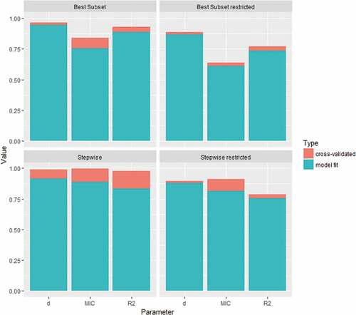
All the statistical measures of agreement between observed and predicted considered rendered most modelling alternatives reliable. Table 1 compares the results from different prediction method alternatives. The values of all measures have been expressed in per-cent units, with the intention to use them for interpreting the proportion of variance in the observed values that is explained by the model predictions, as $R^2$ is interpreted. It is worth noting the high values obtained by the unrestricted version of the step-wise selection, which unrealistically resulted in an over-parameterised model with $p=23$ predictors in spite of the use of AIC. Figure 1 shows bar plots comparing the results for parametric power models, according to whether they included or lacked the overfitting restrictions to variable selection. The versions which restricted the overfitting were more realistic. Willmott’s $d$ showed less contrast among methods than $R^2$ or $MIC$. It also showed lesser differences between values obtained using the whole dataset and cross-validated results.

Table 1. Comparison of diagnoses for different modelling methods and variable selection alternatives to obtain above-ground biomass ($AGB$, Mg·ha⁻¹) predictions

		Best-subset	Best-subset restricted overfitting	Step-wise	Step-wise restricted overfitting	MSN restricted overfitting
Number of predictors* (p)		8	2	23	2	5
Pre./Obs. agreement	$R_{fit}^2$ (%)	93.1	77.0	98.0	78.9	69.4
	$R_{cv}^2$ (%)	88.9	73.4	83.6	75.7	76.3
	$d^{fit}$ (%)	96.6	88.6	99.0	89.5	77.7
	$d^{cv}$ (%)	94.5	86.9	91.7	88.0	81.0
	$MI{C}^{fit}$ (%)	84.2	63.9	99.9	91.2	74.4
	$MI{C}^{cv}$ (%)	75.5	61.0	88.8	81.3	66.4

MSN: most similar neighbour. $R_{fit}^2$: residual coefficient of determination (Equation (1)(1) $\begin{array}{r}{R}^2=1-\left[{\sum }_{i=1}^n{\left(pr{e}_i-ob{s}_i\right)}^2/{\sum }_{i=1}^n{\left(ob{s}_i-\overline{obs}\right)}^2\right]\end{array}$(1) ). $R_{cv}^2$: cross-validated coefficient of determination (Equation (1)(1) $\begin{array}{r}{R}^2=1-\left[{\sum }_{i=1}^n{\left(pr{e}_i-ob{s}_i\right)}^2/{\sum }_{i=1}^n{\left(ob{s}_i-\overline{obs}\right)}^2\right]\end{array}$(1) ). $d^{fit}$: residual Willmott’s index of agreement (Equation (2)(2) $\begin{array}{rl}& d=1-\left[{\sum }_{i=1}^n{\left(pr{e}_i-ob{s}_i\right)}^2\right./\\ & \left.{\sum }_{i=1}^n{\left(\left|pr{e}_i-\overline{obs}\right|+\left|ob{s}_i-\overline{obs}\right|\right)}^2\right]\end{array}$(2) ). $d^{cv}$: cross-validated Willmott’s index of agreement (Equation (2)(2) $\begin{array}{rl}& d=1-\left[{\sum }_{i=1}^n{\left(pr{e}_i-ob{s}_i\right)}^2\right./\\ & \left.{\sum }_{i=1}^n{\left(\left|pr{e}_i-\overline{obs}\right|+\left|ob{s}_i-\overline{obs}\right|\right)}^2\right]\end{array}$(2) ). $MI{C}^{fit}$: residual maximal information coefficient (Equation (6)(6) $MIC=\underset{P,O_{total}<B}{max}\left\{MI\left(P,O\right)/log\left[min\left(P,O\right)\right]\right\}$(6) ). $d^{cv}$: cross-validated maximal information coefficient (Equation (6)(6) $MIC=\underset{P,O_{total}<B}{max}\left\{MI\left(P,O\right)/log\left[min\left(P,O\right)\right]\right\}$(6) ). Coefficients have been multiplied by 100 to yield percentage units.

*The actual predictors selected with each method are detailed in Appendix A.

Figure 1. Comparison of results for alternative statistics of agreement – Willmott’s (1981) index of agreement ($d$), maximal information coefficient ($MIC$; Reshef et al., 2011) and coefficient of determination (R²) – for power models with various variable selection methods, including versus lacking the overfitting restrictions (Valbuena et al., 2017a)

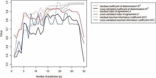
The effects of increasing $p$ in MSN predictions are expressed in Figure 2. The cross-validated coefficients of agreement ranged $R_{cv}^2=63.7-87.1\mathrm{\%}$ for $p=5-28$, however dropping as low as $R_{cv}^2=33.1\mathrm{\%}$ for $p=30$ or $R_{cv}^2=38.7\mathrm{\%}$ for $p=2$. Results in Figure 2 suggest that for small $p$ there may be little divergence whether coefficients of determination are obtained from the model fit $R_{fit}^2$ or cross-validated values $R_{cv}^2$. Willmott’s index of agreement $d$ showed similar patterns as $R_{cv}^2$ (Figure 2), and they were highly correlated $\rho \left(d^{cv},R_{cv}^2\right)=0.99$. This was not the case for $MI{C}^{cv}$ $(\rho \left(MI{C}^{cv},R_{cv}^2\right)=0.65)$, which was, therefore, less redundant than $d$. The difference between non-cross-validated and cross-validated results was, in general, more pronounced for $R^2$ or $MIC$ than for $d$, for the parametric models (Figure 1) as well as for the various MSN predictions (Figure 2).

Figure 2. Evolution of measures of agreement between observed and predicted by most similar neighbour (MSN) method for increasing the number of predictors ($p$). Dashed lines show values obtained using the whole training dataset, whereas solid lines were yielded by cross-validated predictions

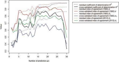
In light of the results obtained in Figure 2, we deduced that $d^{cv}$ was systematically higher than $R_{cv}^2$, ranging as much as $d=59.2-93.8\mathrm{\%}$ for all $p=1-30$. Hence, the proportion of explained variance may simply seem larger when using $d$ instead of $R^2$. For this reason, we further investigated the convenience of using the alternative formulations for Willmott’s index of agreement – $d_1$ and $d_r$ –, which are all compared in Figure 3. Results were again either just lower or higher, but still redundant to the information already provided by $R^2$, since $\rho \left(d_1^{cv},R_{cv}^2\right)=0.99$ and $\rho \left(d_r^{cv},R_{cv}^2\right)=0.98$. Moreover, the latest refined version of Willmott’s index – $d_r^{cv}$ –, showed less contrast among alternatives than $R_{cv}^2$, i.e. with smoother fluctuations along increasing $p$, which rendered it less useful to discriminate the reliability of predictions. Also, when fitting the whole training dataset with very high $p$ these modified versions – $d_1^{fit}$ and $d_r^{fit}$ – obtained very low values, which seems unfair in light of the results obtained by $R_{fit}^2$, $d^{fit}$ and $MI{C}^{fit}$ for $p>22$ in Table 1.

Figure 3. Comparison of the different versions of Willmott’s index of agreement between observed and predicted (Willmott et al., 1985, 2012; Willmott & Wicks, 1980) against the coefficient of determination $R^2$, when the most similar neighbour (MSN) method increased the number of predictors ($p$). Dashed lines show values obtained using the whole training dataset, whereas solid lines were yielded by cross-validated predictions

Discussion

In studies carrying out remote sensing $AGB$ predictions, the most popular statistic employed to evaluate the agreement between observed and predicted is undoubtedly $R^2$ (e.g. Bright et al., 2012; Chen & Zhu, 2013; d’Oliveira et al., 2012; Erdody & Moskal, 2010; Hudak et al., 2006; Latifi et al., 2015; McInerney et al., 2010; Næsset, 2002; Straub, Tian, Seitz, & Reinartz, 2013; Valbuena et al., 2014; Wing et al., 2012; Zhao, Popescu, & Nelson, 2009). It is, however, well known that in presence of bias, $R^2$ may be high despite a poor correspondence between observed and predicted (see, e.g., Valbuena et al., 2014; White, Coops, & Scott, 2000). For this reason, it has been argued that $R^2$ may not necessarily be related to the accuracy of predictions (Paruelo et al., 1998), and hence Willmott’s (1981) $d$ has been suggested as a more appropriate alternative to evaluate remote sensing predictions (Almeida et al., 2016; García et al., 2010; Yebra & Chuvieco, 2009), in line with discussions held in the broader realm of statistical modelling (Fox, 1981; Willmott, 1982). In our results, however, we observed an underperformance of $d$ as a statistic truly expressing the degree of agreement between observed and predicted. Even having been obtained after cross-validation, values of $d$ summarized in Table 1 and Figure 1 were quite large in all cases, regardless of results in other measures of model performance (see Valbuena et al., 2017a). On the other hand, $R_{cv}^2$ obtained sounder results which were more likely to discriminate reliable from unreliable alternatives, whereas Figure 2 shows that $d$ may simply yield values systematically larger than $R_{cv}^2$. The modifications to $d$ did not necessarily overcome this problem, since Willmott et al.’s (1985) $d_1$ was instead systematically lower than $R^2$, and the more recent Willmott et al.’s (2012) $d_r$ showed similar but smoother patterns of variation (Figure 3). As a conclusion, we suggest that $R^2$ may be a better alternative than $d$, in light of our results. Although Willmott (1981) correctly affirmed that $R^2$ may show large values if predictions are evenly distributed through the range but yet biased, we suggest that $R_{cv}^2$ may simply be used along with a hypothesis test ensuring the absence of bias, such as those proposed by Piñeiro et al. (2008).

Willmott’s (1981, 1982) put forward a number of arguments in favour of using $d$, and many of them point out that $d$ may be conceptually superior to $R^2$ for describing the agreement in the observed versus predicted relationship for model evaluation (García et al., 2010; Yebra & Chuvieco, 2009). One interesting remark arises when comparing the calculation of Willmott’s (1981) index $d$ of agreement with that for Pearson’s sample correlation coefficient $r$. It is noteworthy to mention that, although $R^2$ expresses the proportion of variance in the dependent variable explained by a model while $r$ the dependence between two variables, $R^2$ and $r$ are closely related to one another. 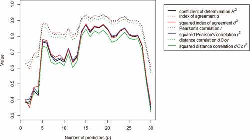In particular, $R^2$ is equivalent to the square of Pearson’s correlation ($r^2$) when using a simple linear regression with intercept fit. Although this equivalence is not valid for MSN, we explored the possibility that $R^2$ and $r^2$ may be fairly close by analogy. Figure 4 shows that was indeed the case, as it was also for the square of Willmott’s index of agreement ($d^2$). Thus, we argue that studies with a particular interest in using Willmott’s (1981, 1982) suggestions for evaluating model predictions (Almeida et al., 2016; García et al., 2010; Grzegozewski et al., 2016; Wachholz de Souza et al., 2015; Yebra & Chuvieco, 2009) should report $d^2$ instead, in order to make it more comparable to more widespread studies using $R^2$ (e.g. Næsset, 2002, 2004; Hudak et al., 2006; Zhao et al., 2009; Erdody & Moskal, 2010; McInerney et al., 2010; Bright et al., 2012; d’Oliveira et al., 2012; Wing et al., 2012; Chen & Zhu, 2013; Straub et al., 2013; Asner & Mascaro, 2014; Valbuena et al., 2014; Latifi et al., 2015; Zolkos et al., 2013).

Figure 4. Comparison of original versions of Willmott’s index of agreement $d$ and other measures of correlation (dashed lines), and their squared versions (solid lines) against the coefficient of determination $R^2$

The case of using maximal information coefficient (Reshef et al., 2011) could also be supported by analogy to the relationship between $R^2$ and $r^2$, since $MIC$ is usually regarded as a non-parametric version of correlation (Chen & Yang, 2016; Görgens et al., 2017; Thomas et al., 2017; Vallières et al., 2017). Results for $MIC$ in Table 1 and Figure 2 can be best interpreted by observing the scatterplots of observed versus cross-validated predictions published in Valbuena et al. (2017a: Figures 2–3). The remarkably higher values of $MIC$ with respect to $R^2$ for, e.g., $p=8$ or $p=10$ (Figure 2), can be explained by the fact that these scatterplots show clustered cases in the observed versus predicted metric space (see Valbuena et al., 2017a: Figure 2). In that sense, we deduct that $MIC$ simply favours local clustering of predictions, whether or not they correspond to the observations. We, therefore, discourage the use of $MIC$ as a substitute of $R^2$ for model evaluation. Since Simon and Tibshirani (2011) recommended the use of distance correlation $dCor$ (Székely & Rizzo, 2017) as an alternative to $MIC$, we also included it in Figure 4. The analogy of squaring $d$ does not work for $MIC$, which simply showed unrealistically low values when squared. The square of distance correlation ($dCo{r}^2$), however, also obtained values which were fairly similar to those for $R^2$ (Figure 4).

Another unexpected result obtained in Figure 2 was the fact that differences between $R_{fit}^2$ and $R_{cv}^2$ only became apparent for large $p$, even for such a small $n$ as it was employed in our study case. This result suggests that, in spite of the popularity of cross-validation in the assessment of forest $AGB$ using remote sensing (e.g. Franco-Lopez et al., 2001; García et al., 2010; Hudak et al., 2006; Hudak, Crookston, Evans, Hall, & Falkowski, 2008; Latifi et al., 2015; McInerney et al., 2010; McRoberts et al., 2002; Næsset, 2002; Packalén & Maltamo, 2008; Valbuena et al., 2013a; Wing et al., 2012), reports on results obtained by leave-one-out cross-validation could easily converge to those yielded by the model fit (i.e. using the same dataset for training and validation). This may put into question the need for cross-validation at all since it makes little difference for those models with more realistic number of predictors $\left(p\le 3-5\right)$ (Figure 2). Although cross-validation may add robustness to an analysis with small sample sizes and few highly influential cases, our results show little difference compared to using the entire training dataset (Valbuena et al., 2017a). Future research should be devoted to further investigating the reliability of cross-validation, accounting for trade-offs between model generality and statistical power (Cohen et al., 2003) faced when pondering between using cross-validation or separating part of the available field information for independent model validation. It is useful for practical forest inventory to mention that models restricted according to Valbuena et al. (2017a), despite using less predictor variables, obtained similar performances in light of all the accuracy assessment figures analysed.

Conclusions

These are the conclusions that can be drawn from the results obtained in this study and their subsequent discussion. First, we observed an underperformance of Willmott’s (1981) $d$ in comparison to $R^2$, since the latter was more sensitive to actual model performance. Second, the refinements later introduced to that same index (Willmott et al., 1985, 2012) did not solve the observed shortcomings either. Third, we wish to put forward a recommendation to use a squared version of Willmott’s index $d^2$ for those who prefer it above $R^2$, to allow better comparison with studies using $R^2$. Fourth, the maximal information coefficient $MIC$ is not at all suitable for comparing relationships between observed and predicted in model evaluation. And finally, for a small number of predictors, the difference between using cross-validation or not using it at all can be negligible, which shows how useful can be its comparison for evaluating overfitting. More research would be needed to explore the usefulness of different cross-validation alternatives in the specific topic of remote sensing predictions of forest $AGB$.

Acknowledgments

This work was partially supported by the Spanish Directorate General for Scientific and Technical Research under Grant CGL2013-46387-C2-2-R. We also thank the Valsain Forest Centre, of the National Park Body (Spain), and Prof. David A. Coomes (University of Cambridge) for their valuable help. Dr Valbuena’s work is supported by an EU Horizon 2020 Marie Sklodowska-Curie Action entitled “Classification of forest structural types with LIDAR remote sensing applied to study tree size-density scaling theories” (LORENZLIDAR-658180). Danilo Almeida acknowledges support from São Paulo Research Foundation (FAPESP) (grant 2018/21338-3).

Disclosure statement

No potential conflict of interest was reported by the authors.

Additional information

Funding

This work was supported by the Spanish Directorate General for Scientific and Technical Research [Grant CGL2013-46387-C2-2-R]; EU Horizon 2020 Marie Sklodowska-Curie Action [LORENZLIDAR-658180]; São Paulo Research Foundation (FAPESP) [grant 2018/21338-3].

Appendices

Appendix A. Details on the predictors selected by each of these methods. These models were the same detailed in Valbuena et al. (2017a)

Best-subset	Best-subset restricted overfitting	Step-wise	Step-wise restricted overfitting	MSN restricted overfitting
H.GC	H.mean	H.GC	H.P75	H.L2
H.L3	NDVI.P75	H.CV	H.L3	H.L3
H.Mean		NDVI.GC		H.AAD
H.P95		H.L2		H.Mean
H.IQR		H.L4		H.GC
H.P40		H.L3
NDVI.Var		H.AAD
NDVI.AAD		H.Mean
		H.SD
		H.Kurt
		H.P90
		H.P95
		H.P80
		H.P75
		NDVI.SD
		NDVI.AAD
		NDVI.L1
		NDVI.L3
		NDVI.P25
		NDVI.P05
		NDVI.P75
		NDVI.P70
		NDVI.Var

Descriptors of predictor variables are detailed in Manzanera et al. (2016) and Valbuena et al (2017b). Names are composed of a prefix and a suffice separated by a dot (.). Prefices refer to the attribute characteristic used: height from LIDAR sensor (H) or normalized vegetation index from multispectral sensor (NDVI). Suffices refer to the statistical descriptor of the distribution of that attribute characteristic: mean (Mean), variance (Var), standard deviation (SD), average absolute deviation (AAD), percentiles (P05, P25, P40, P70, P75, P80, P90, P95), L-moments (L1, L2, L3, L4), Gini coefficient (GC), inter-quartile range (IQR).

References

- Adnan, S., Maltamo, M., Coomes, D.A., García-Abril, A., Malhi, Y., Manzanera, J.A., … Valbuena, R. (2019). A simple approach to forest structure classification using airborne laser scanning that can be adopted across bioregions. Forest Ecology and Management, 433, 111–121. doi:10.1016/j.foreco.2018.10.057
- Agrawal, A., Nepstad, D., & Chhatre, A. (2011). Reducing emissions from deforestation and forest degradation. Annual Review of Environmental Resources, 36, 373–396. doi:10.1146/annurev-environ-042009-094508
- Almeida, D.R.A., Nelson, B.W., Schietti, J., Görgens, E.B., Resende, A.F., Stark, S.C., & Valbuena, R. (2016). Contrasting fire damage and fire susceptibility between seasonally flooded forest and upland forest in the Central Amazon using portable profiling LiDAR. Remote Sensing of Environment, 184, 153–160. doi:10.1016/j.rse.2016.06.017
- Aschonitis, V.G., Papamichail, D., Demertzi, K., Colombani, N., Mastrocicco, M., Ghirardini, A., … Fano, E.A. (2017). High resolution global grids of revised Priestley-Taylor and Hargreaves-Samani coefficients for assessing ASCE-standardized reference crop evapotranspiration and solar radiation. Earth System Science Data, 9(2), 615–638. doi:10.5194/essd-9-615-2017
- Asner, G.P. (2009). Tropical forest carbon assessment: Integrating satellite and airborne mapping approaches. Environmental Research Letters, 4, 034009. doi:10.1088/1748-9326/4/3/034009
- Asner, G.P. (2011). Painting the world REDD: Addressing scientific barriers to monitoring emissions from tropical forests. Environmental Research Letters, 6, 021002. doi:10.1088/1748-9326/6/2/021002
- Asner, G.P., & Mascaro, J. (2014). Mapping tropical forest carbon: Calibrating plot estimates to a simple LiDAR metric. Remote Sensing of Environment, 140, 614–624. doi:10.1016/j.rse.2013.09.023
- Baskerville, G. (1972). Use of logarithmic regression in the estimation of plant biomass. Canadian Journal of Forest Research, 2, 49–53. doi:10.1139/x72-009
- Basuki, T.M., van Laake, P.E., Skidmore, A.K., & Hussin, Y.A. (2009). Allometric equations for estimating the above-ground biomass in tropical lowland Dipterocarp forests. Forest Ecology and Management, 257(8), 1684–1694. doi:10.1016/j.foreco.2009.01.027
- Bottalico, F., Chirici, G., Giannini, R., Mele, S., Mura, M., Puxeddu, M., … Travaglini, D. (2017). Modeling Mediterranean forest structure using airborne laser scanning data. International Journal of Applied Earth Observation and Geoinformation, 57, 145–153. doi:10.1016/j.jag.2016.12.013
- Bright, B.C., Hicke, J.A., & Hudak, A.T. (2012). Estimating aboveground carbon stocks of a forest affected by mountain pine beetle in Idaho using lidar and multispectral imagery. Remote Sensing of Environment, 124, 270–281. doi:10.1016/j.rse.2012.05.016
- Bring, A., & Destouni, G. (2014). Arctic climate and water change: Model and observation relevance for assessment and adaptation. Surveys in Geophysics, 35, 853e877. doi:10.1007/s10712-013-9267-6
- Burnham, K.P., & Anderson, D.R. (2002). Model selection and multimodel inference: a practical information-theoretic approach, (2nd ed.). Secaucus, NJ: Springer.
- Chave, J., Andalo, C., Brown, S., Cairns, M.A., Chambers, J.Q., Eamus, D., … & Lescure, J. P. (2005). Tree allometry and improved estimation of carbon stocks and balance in tropical forests. Oecologia, 145(1), 87–99. doi:10.1007/s00442-005-0100-x
- Chave, J., Condit, R., Aguilar, S., Hernandez, A., Lao, S., & Perez, R. (2004). Error propagation and scaling for tropical forest biomass estimates. Philosophical Transactions of the Royal Society of London B: Biological Sciences, 359(1443), 409–420. doi:10.1098/rstb.2003.1425
- Chave, J., Réjou-Méchain, M., Búrquez, A., Chidumayo, E., Colgan, M.S., Delitti, W.B.C., … & Henry, M. (2014). Improved allometric models to estimate the aboveground biomass of tropical trees. Global Change Biology, 20, 3177–3190. doi:10.1111/gcb.12629
- Chen, Y., & Yang, H. (2016). A novel information-theoretic approach for variable clustering and predictive modeling using dirichlet process mixtures. Scientific Reports, 6, 38913. doi:10.1038/srep38913
- Chen, Y., & Zhu, X. (2013). An integrated GIS tool for automatic forest inventory estimates of Pinus radiata from LiDAR data. GIScience & Remote Sensing, 50, 667–689. doi:10.1080/15481603.2013.866783
- Clark, D.B., & Kellner, J.R. (2012). Tropical forest biomass estimation and the fallacy of misplaced concreteness. Journal of Vegetation Science, 23(6), 1191–1196.
- Cohen, W.B., Maiersperger, T.K., Gower, S.T., & Turner, D.P. (2003). An improved strategy for regression of biophysical variables and Landsat ETM+. Remote Sensing of Environment, 84, 561–571. doi:10.1016/S0034-4257(02)00173-6
- Coomes, D., Dalponte, M., Jucker, T., Asner, G.P., Banin, L.F., Burslem, D.F.R.P., … Qie, L. (2017). Area-based vs tree-centric approaches to mapping forest carbon in Southeast Asian forests from airborne laser scanning data. Remote Sensing of Environment, 194, 77–88. doi:10.1016/j.rse.2017.03.017
- Crookston, N.L., & Finley, A.O. (2007). YaImpute: An R package for κNN imputation. Journal of Statistical Software, 23(10), 1–16.
- Cuny, H.E., Rathgeber, C.B.K., Frank, D., Fonti, P., Mã¤Kinen, H., Prislan, P., et al. (2015). Woody biomass production lags stem-girth increase by over one month in coniferous forests. Nature Plants, 10/26(1), 15160. doi:10.1038/nplants.2015.160
- d‘Oliveira, M.V.N., Reutebuch, S.E., McGaughey, R.J., & Andersen, H.E. (2012). Estimating forest biomass and identifying low-intensity logging areas using airborne scanning lidar in Antimary State Forest, Acre State, Western Brazilian Amazon. Remote Sensing of Environment, 124, 479–491. doi:10.1016/j.rse.2012.05.014
- Domingo, D., Lamelas, M.T., Montealegre, A.L., García-Martín, A., & de la Riva, J. (2018). Estimation of total biomass in aleppo pine forest stands applying parametric and nonparametric methods to low-density airborne laser scanning data. Forests, 9, 158. doi:10.3390/f9040158
- Domingo, D., Lamelas-Gracia, M.T., Montealegre-Gracia, A.L., & de la Riva-Fernández, J. (2017). Comparison of regression models to estimate biomass losses and CO2 emissions using low-density airborne laser scanning data in a burnt Aleppo pine forest. European Journal of Remote Sensing, 50, 384–396. doi:10.1080/22797254.2017.1336067
- Duveiller, G., Fasbender, D., & Meroni, M. (2016). Revisiting the concept of a symmetric index of agreement for continuous datasets. Scientific Reports, 6, 19401. doi:10.1038/srep19401
- Egberth, M., Nyberg, G., Naesset, E., Gobakken, T., Mauya, E., Malimbwi, R., et al. (2017). Combining airborne laser scanning and Landsat data for statistical modeling of soil carbon and tree biomass in Tanzanian Miombo woodlands. Carbon Balance and Management, 12, 8. doi:10.1186/s13021-017-0076-y
- Eggleston, H.S., Buendia, L., Miwa, K., Ngara, T., & Tanabe, K. (2006). IPCC guidelines for national greenhouse gas inventories. Institute for Global Environmental Strategies. Japan :IGES.
- Ehrenberg, A.S.C. (1982). How good is best? Journal of the Royal Statistical Society, Series A, 145, 364–366. doi:10.2307/2981869
- Erdody, T.L., & Moskal, L.M. (2010). Fusion of LiDAR and imagery for estimating forest canopy fuels. Remote Sensing of Environment, 114, 725−737. doi:10.1016/j.rse.2009.11.002
- Eskelson, B.N.I., Temesgen, H., Lemay, V., Barrett, T.M., Crookston, N.L., & Hudak, A.T. (2009). The roles of nearest neighbor methods in imputing missing data in forest inventory and monitoring databases. Scandinavian Journal of Forest Research, 24, 235–246. doi:10.1080/02827580902870490
- Estornell, J., Ruiz, L.A., Velázquez-Martí, B., & Hermosilla, T. (2011). Analysis of the factors affecting LiDAR DTM accuracy in a steep shrub area. International Journal of Digital Earth, 4, 521–538. doi:10.1080/17538947.2010.533201
- Estornell, J., Ruiz, L.A., Velázquez-Martí, B., & Hermosilla, T. (2012). Estimation of biomass and volume of shrub vegetation using LiDAR and spectral data in a Mediterranean environment. Biomass and Bioenergy, 46, 710–721. doi:10.1016/j.biombioe.2012.06.023
- Filosi, M., Visintainer, R., & Albanese, D. (2014). Minerva: Maximal information-based nonparametric exploration. R Package Version 1.4.1.
- Fox, D.G. (1981). Judging air quality model performance. Bulletin of the American Meteorolical Society, 62, 599–609. doi:10.1175/1520-0477(1981)062<0599:JAQMP>2.0.CO;2
- Franco-Lopez, H., Ek, A.R., & Bauer, M.E. (2001). Estimation and mapping of forest stand density, volume, and cover type using the k-nearest neighbors method. Remote Sensing of Environment, 77(3), 251–274. doi:10.1016/S0034-4257(01)00209-7
- Gaitan, C.F., Hsieh, W.W., & Cannon, A.J. (2014). Comparison of statistically downscaled precipitation in terms of future climate indices and daily variability for southern Ontario and Quebec, Canada. Climate Dynamics, 43, 3201e3217. doi:10.1007/s00382-014-2098-4
- Ganpule, S., Daphalapurkar, N.P., Ramesh, K.T., Knutsen, A.K., Pham, D.L., Bayly, P.V., & Prince, J.L. (2017). A three-dimensional computational human head model that captures live human brain dynamics. Journal of Neurotrauma, 34(13), 2154. doi:10.1089/neu.2016.4503
- García, M., Riaño, D., Chuvieco, E., & Danson, F.M. (2010). Estimating biomass carbon stocks for a Mediterranean forest in central Spain using LiDAR height and intensity data. Remote Sensing of Environment, 115, 1369–1379. doi:10.1016/j.rse.2011.01.017
- Garcia-Gutierrez, J., Gonzalez-Ferreiro, E., Riquelme-Santos, J.C., Miranda, D., Dieguez-Aranda, U., & Navarro-Cerrillo, R.M. (2014). Evolutionary feature selection to estimate forest stand variables using LiDAR. International Journal of Applied Earth Observation and Geoinformation, 26, 119–131. doi:10.1016/j.jag.2013.06.005
- García-Gutiérrez, J., Martínez-Álvarez, F., Troncoso, A., & Riquelme, J.C. (2015). A comparison of machine learning regression techniques for LiDAR-derived estimation of forest variables. Neurocomputing, 167, 24–31. doi:10.1016/j.neucom.2014.09.091
- Goetz, S.J., & Dubayah, R.O. (2014). Advances in remote sensing technology and implications for measuring and monitoring forest carbon stocks and change. Carbon Management, 2, 231–244. doi:10.4155/cmt.11.18
- Gómez, C., Alejandro, P., Hermosilla, T., Montes, F., Pascual, C., Ruiz, L.A., … Valbuena, R. (2019). Remote sensing for the Spanish forests in the 21st century: A review of advances, needs, and opportunities. Forest Systems, 28(1), eR002. doi:10.5424/fs/2019281-14221
- González-Ferreiro, E., Dieguez-Aranda, U., & Miranda, D. (2012). Estimation of stand variables in Pinus radiata D. Don plantations using different LiDAR pulse densities. Forestry, 85, 281–292. doi:10.1093/forestry/cps002
- González-Olabarria, J.-R., Rodríguez, F., Fernández-Landa, A., & Mola-Yudego, B. (2012). Mapping fire risk in the model forest of Urbión (Spain) based on airborne LiDAR measurements. Forest Ecology and Management, 282, 149–156. doi:10.1016/j.foreco.2012.06.056
- Görgens, E.B., Valbuena, R., & Rodríguez, L.C. (2017). A method for optimizing height threshold when computing airborne laser scanning metrics. Photogrammetric Engineering and Remote Sensing, 83(5), 343–350. doi:10.14358/PERS.83.5.343
- Grzegozewski, D.M., Johann, J.A., Uribe-Opazo, M., Mercante, E., & Coutinho, A.C. (2016). Mapping soya bean and corn crops in the State of Paraná, Brazil, using EVI images from the MODIS sensor. International Journal of Remote Sensing, 37, 1257–1275. doi:10.1080/01431161.2016.1148285
- Guerra-Hernández, J., Görgens, E.B., García-Gutiérrez, J., Carlos, L., Rodriguez, E., Tomé, M., & González-Ferreiro, E. (2016). Comparison of ALS based models for estimating aboveground biomass in three types of Mediterranean forest. European Journal of Remote Sensing, 49, 185–204. doi:10.5721/EuJRS20164911
- Hansen, M.C., Potapov, P.V., Moore, R., Hancher, M., Turubanova, S.A.A., Tyukavina, A., … & Kommareddy, A. (2013). High-resolution global maps of 21st-century forest cover change. Science, 342, 850–853. doi:10.1126/science.1244693
- Hernando, A., Puerto, L., Mola-Yudego, B., Manzanera, J., García-Abril, A., Maltamo, M., & Valbuena, R. (2019). Estimation of forest biomass components through airborne LiDAR and multispectral sensors. iForest- Biogeosciences and Forestry, 12, 207–213.doi:10.3832/ifor2735-012
- Hudak, A.T., Crookston, N.L., Evans, J.S., Falkowski, M.J., Smith, A.M.S., Gessler, P.E., … Morgan, P. (2006). Regression modeling and mapping of coniferous forest basal area and tree density from discrete-return lidar and multispectral satellite data. Canadian Journal of Remote Sensing, 32, 126–138. doi:10.5589/m06-007
- Hudak, A.T., Crookston, N.L., Evans, J.S., Hall, D.E., & Falkowski, M.J. (2008). Nearest neighbor imputation of species-level, plot-scale forest structure attributes from LiDAR data. Remote Sensing of Environment, 112(5), 2232–2245. doi:10.1016/j.rse.2007.10.009
- Iais, P.C., Bombelli, A., Williams, M., Piao, S.L., Chave, J., Ryan, C.M., et al. (2011). The carbon balance of Africa: Synthesis of recent research studies. Philosophical Transactions of the Royal Society A, 369(1943), 2038–2057. doi:10.1098/rsta.2010.0328
- Ibrom, A., Oltchev, A., June, T., Ross, T., Kreilein, H., & Falk, U. (2007). Effects of land-use change on matter and energy exchange between ecosystems in the rain forest margin and the atmosphere. In T. Tscharntke, C. Leuschner, M. Zeller, E. Guhardja, A. Bidin, et al. (Eds.), Stability of tropical rainforest margins: Linking ecological, economic and social constraints of land use and conservation (pp. 461–490). Berlin, Heidelberg: Springer Berlin Heidelberg.
- Krainovic, P., Almeida, D., & Sampaio, P. (2017). New allometric equations to support sustainable plantation management of Rosewood (Aniba rosaeodora Ducke) in the Central Amazon. Forests, 8(9), 327. doi:10.3390/f8090327
- Latifi, H., Heurich, M., Hartig, F., Müller, J., Krzystek, P., Jehl, H., & Dech, S. (2015). Estimating over- and understorey canopy density of temperate mixed stands by airborne LiDAR data. Forestry, 89(1), 69–81. doi:10.1093/forestry/cpv032
- Legates, D.R., & McCabe, G.J., Jr. (1999). Evaluating the use of “goodness-of-fit” measures in hydrologic and hydroclimatic model validation. Water Resources Research, 35(1), 233–241. doi:10.1029/1998WR900018
- Linfoot, E.H. (1957). An informational measure of correlation. Information and Control, 1, 85–89. doi:10.1016/S0019-9958(57)90116-X
- Lipovetsky, S. (2013). How good is best? Multivariate case of Ehrenberg-Weisberg analysis of residual errors in competing regressions. Journal of Modern Applied Statistical Methods, 12(2), 14. doi:10.22237/jmasm/1383279180
- Loew, A., Bell, W., Brocca, L., Bulgin, C.E., Burdanowitz, J., Calbet, X., … Schröder, M. (2017). Validation practices for satellite based earth observation data across communities. Reviews of Geophysics, 55, 779–817. doi:10.1002/2017RG000562
- López-Moreno, J.I., Latron, J., & Lehmann, A. (2010). Effects of sample and grid size on the accuracy and stability of regression-based snow interpolation methods. Hydrological Processes, 24, 1914–1928.
- Lumley, T., & Miller, A. (2009). Leaps: Regression Subset Selection (R package version2.9) https://CRAN.R-project.org/package=leaps.
- Mallows, C.L. (1973). Some comments on Cp. Technometrics, 15 (4), 661–675.
- Manzanera, J.A., Garcia-Abril, A., Pascual, C., Tejera, R., Martín Fernández, S., Tokola, T., & Valbuena, R. (2016). Fusion of airborne LiDAR and multispectral sensors reveals synergic capabilities in forest structure characterization. GIScience & Remote Sensing, 53, 723–738. doi:10.1080/15481603.2016.1231605
- Marshall, A.R., Willcock, S., Platts, P.J., Lovett, J.C., Balmford, A., Burgess, N.D., … & Lewis, S.L. (2012). Measuring and modelling above-ground carbon and tree allometry along a tropical elevation gradient. Biological Conservation, 154, 20–33. doi:10.1016/j.biocon.2012.03.017
- McInerney, D.O., Suárez, J., Valbuena, R., & Nieuwenhuis, M. (2010). Forest canopy height retrieval using Lidar data, medium-resolution satellite imagery and kNN estimation in Aberfoyle, Scotland. Forestry, 83(2), 195–206. doi:10.1093/forestry/cpq001
- McRoberts, R.E., Nelson, M.D., & Wendt, D.G. (2002). Stratified estimation of forest area using satellite imagery, inventory data, and the k-nearest neighbors technique. Remote Sensing of Environment, 82(2–3), 457–468. doi:10.1016/S0034-4257(02)00064-0
- Miller, A. (1984). Selection of subsets of regression variables. Journal of the Royal Statistical Society, Series A, 147, 389–425. doi:10.2307/2981576
- Molto, Q., Rossi, V., & Blanc, L. (2013). Error propagation in biomass estimation in tropical forests. Methods in Ecology and Evolution / British Ecological Society, 4(2), 175–183. doi:10.1111/j.2041-210x.2012.00266.x
- Montealegre, A.L., Lamelas, M.T., de la Riva, J., García-Martín, A., & Escribano, F. (2016). Use of low point density ALS data to estimate stand-level structural variables in Mediterranean Aleppo pine forest. Forestry, 89, 373–382. doi:10.1093/forestry/cpw008
- Montealegre, A.L., Lamelas-Gracia, M.T., García-Martín, A., de la Riva-Fernández, J., & Escribano-Bernal, F. (2017). Using low-density discrete airborne laser scanning data to assess the potential carbon dioxide emission in case of a fire event in a Mediterranean pine forest. GIScience & Remote Sensing, 54, 721–740. doi:10.1080/15481603.2017.1320863
- Montero, G., Ruiz-Peinado, R., & Muñoz, M. (2005). Producción de biomasa y fijación de CO2 por los bosques españoles. Madrid, Spain (in Spanish): Monografías Instituto Nacional de Investigación y Tecnología Agraria y Alimentaria, Serie Forestal.
- Morsy, M., El-Sayed, T., & Ouda, S.A.H. (2016). Potential evapotranspiration under present and future climate. In S.A.H. Ouda & A.E. Zohry (Eds.), Management of climate induced drought and water scarcity in Egypt: Unconventional solutions (pp. 5–25). Cham: Springer International Publishing.
- Murrell, B., Murrell, D., & Murrell, H. (2014). R2-equitability is satisfiable. Proceedings of the National Academy of Sciences, 111, E2160–E2160 10.1073/pnas.1403623111
- Næsset, E. (2002). Predicting forest stand characteristics with airborne scanning laser using a practical two-stage procedure and field data. Remote Sensing of Environment, 801, 88–99. doi:10.1016/S0034-4257(01)00290-5
- Næsset, E. (2004). Estimation of above-and below-ground biomass in boreal forest ecosystems. In M. Thies, B. Koch, H. Spiecker, & H. Weinacker (Eds.), Laser-scanners for forest and landscape assessment (Vol. (2004), pp. 145–148). Freiburg, Germany: International Society for Photogrammetry and Remote Sensing.
- Nendel, C., Venezia, A., Piro, F., Ren, T., Lillywhite, R., & Rahn, C.C. (2013). The performance of the EU-Rotate_N model in predicting the growth and nitrogen uptake of rotations of field vegetable crops in a Mediterranean environment. Journal of Agricultural Science, 151(4), 538–555. doi:10.1017/S0021859612000688
- Oyler, J.W., Ballantyne, A., Jencso, K., Sweet, M., & Running, S.W. (2015). Creating a topoclimatic daily air temperature dataset for the conterminous United States using homogenized station data and remotely sensed land skin temperature. International Journal of Climatology, 35, 2258e2279. doi:10.1002/joc.4127
- Packalén, P., & Maltamo, M. (2008). Estimation of species-specific diameter distributions using airborne laser scanning and aerial photographs. Canadian Journal of Forest Research, 38(7), 1750–1760. doi:10.1139/X08-037
- Paruelo, J.M., Jobbágy, E.G., Sala, O.E., Lauenroth, W.K., & Burke, I. (1998). Functional and structural convergence of temperate grassland and shrubland ecosystems. Ecological Applications, 8(1), 194–206. doi:10.1890/1051-0761(1998)008[0194:FASCOT]2.0.CO;2
- Piñeiro, G., Perelman, S., Guerschman, J.P., & Paruelo, J.M. (2008). How to evaluate models: Observed vs. predicted or predicted vs. observed? Ecological Modelling, 216(3), 316−322. doi:10.1016/j.ecolmodel.2008.05.006
- R Development Core Team. (2016). R: A language and environment for statistical computing. Vienna, Austria. https://www.R-project.org/.
- Reshef, D.N., Reshef, Y.A., Finucane, H.K., Grossman, S.R., McVean, G., Turnbaugh, P.J., … Sabeti, P.C. (2011). Detecting novel associations in large data sets. Science, 334(6062), 1518–1524. doi:10.1126/science.1205438
- Rizzo, M.L., & Szekely, G.J. (2017). Energy: E-statistics: Multivariate inference via the energy of data. R Package Version 1.7-2.
- Ruiz-Peinado, R., Del Rio, M., & Montero, G. (2011). New models for estimating the carbon sink capacity of Spanish softwood species. Forest Systems, 20, 176–188. doi:10.5424/fs/2011201-11643
- Sawadogo, L., Savadogo, P., Tiveau, D., Dayamba, S.D., Zida, D., Nouvellet, Y., et al. (2010). Allometric prediction of above-ground biomass of eleven woody tree species in the Sudanian savanna-woodland of West Africa. Journal of Forestry Research, 21(4), 475–481. doi:10.1007/s11676-010-0101-4
- Shannon, C.E. (1948). A mathematical theory of communication. The Bell System Technical Journal, 27, 379–423 and 623–656. doi:10.1002/bltj.1948.27.issue-3
- Sileshi, G.W. (2014). A critical review of forest biomass estimation models, common mistakes and corrective measures. Forest Ecology and Management, 10(1), 329, 237–254. doi:10.1016/j.foreco.2014.06.026
- Simon, N., & Tibshirani, R. (2011). Comment on “detecting novel associations in large data set” by Reshef et al. arXiv:1401.7645 [stat.ME]
- Speed, T. (2011). A correlation for the 21st century. Science, 334(6062), 1502–1503. doi:10.1126/science.1215894
- Sprugel, D.G. (1983). Correcting for bias in log-transformed allometric equations. Ecology, 64, 209–210. doi:10.2307/1937343
- Straub, C., Tian, J., Seitz, R., & Reinartz, P. (2013). Assessment of Cartosat-1 and WorldView-2 stereo imagery in combination with a LiDAR-DTM for timber volume estimation in a highly structured forest in Germany. Forestry, 86(4), 463–473. doi:10.1093/forestry/cpt017
- Sugiura, N. (1978). Further analysts of the data by akaike’s information criterion and the finite corrections. Communications in Statistics - Theory and Methods, 7 (1), 13–26.
- Székely, G.J., & Rizzo, M. (2009). Brownian distance covariance. Annals of Applied Statistics, 3(4), 1233–1303.
- Székely, G.J., & Rizzo, M. (2017). The energy of data. Annual Review of Statistics and Its Application, (2017)(4), 447–479. doi:10.1146/annurev-statistics-060116-054026
- Temesgen, H., Affleck, D., Poudel, K., Gray, A., & Sessions, J. (2015, May 19). A review of the challenges and opportunities in estimating above ground forest biomass using tree-level models. Scandinavian Journal of Forest Research, 30(4), 326–335.
- Theil, H. (1958). Economic forecasts and policy. Amsterdam: North Holland.
- Thomas, F., Bordron, P., Eveillard, D., & Michel, G. (2017). Gene expression analysis of zobellia galactanivorans during the degradation of algal polysaccharides reveals both substrate-specific and shared transcriptome-wide responses. Frontiers in Microbiology, 8(1808). doi:10.3389/fmicb.2017.01808
- Tyukavina, A., Hansen, M.C., Potapov, P.V., Stehman, S.V., Smith-Rodriguez, K., Okpa, C., & Aguilar, R. (2017). Types and rates of forest disturbance in Brazilian Legal Amazon, 2000–2013. Science Advances, 3(4), e1601047. doi:10.1126/sciadv.1601047
- UNFCCC - United Nations Framework Convention on Climate Change. (2014). Warsaw Framework for REDD+.
- Valbuena, R., De-Blas, A., Martín-Fernández, S., Maltamo, M., Nabuurs, G.J., & Manzanera, J.A. (2013a). Within-species benefits of back-projecting airborne laser scanner and multispectral sensors in monospecific pinus sylvestris forests. European Journal of Remote Sensing, 46, 491–509. doi:10.5721/EuJRS20134629
- Valbuena, R., Heiskanen, J., Aynekulu, E., Pitkänen, S., & Packalen, P. (2016). Sensitivity of above-ground biomass estimates to height-diameter modelling in mixed-species West African Woodlands. PloS One, 11(7), e0158198. doi:10.1371/journal.pone.0158198
- Valbuena, R., Hernando, A., Manzanera, J.A., Görgens, E.B., Almeida, D.R.A., Mauro, F., … Coomes, D.A. (2017a). Enhancing of accuracy assessment for forest above-ground biomass estimates obtained from remote sensing via hypothesis testing and overfitting evaluation. Ecological Modelling, 622, 15–26. doi:10.1016/j.ecolmodel.2017.10.009
- Valbuena, R., Hernando, A., Manzanera, J.A., Martínez-Falero, E., García-Abril, A., & Mola-Yudego, B. (2017b). Most similar neighbour imputation of forest attributes using metrics derived from combined airborne LIDAR and multispectral sensors. International Journal of Digital Earth. doi:10.1080/17538947.2017.1387183
- Valbuena, R., Maltamo, M., Martín-Fernández, S., Packalén, P., Pascual, C., & Nabuurs, G.J. (2013b). Patterns of covariance between airborne laser scanning metrics and Lorenz curve descriptors of tree size inequality. Canadian Journal of Remote Sensing, 39(2013), S18–S31. doi:10.5589/m13-012
- Valbuena, R., Maltamo, M., & Packalen, P. (2016). Classification of forest development stages from national low-density lidar datasets: a comparison of machine learning methods. Revista De Teledetección – Spanish Journal of Remote Sensing, 45, 15–25. doi:10.4995/raet.2016.4029
- Valbuena, R., Mauro, F., Arjonilla, F., & Manzanera, J.A. (2011). Comparing airborne laser scanning-imagery fusion methods based on geometric accuracy in forested areas. Remote Sensing of Environment, 115, 1942–1954. doi:10.1016/j.rse.2011.03.017
- Valbuena, R., Mauro, F., Rodriguez-Solano, R., & Manzanera, J.A. (2012). Partial least squares for discriminating variance components in global navigation satellite systems accuracy obtained under Scots pine canopies. Forest Science, 582, 139–153. doi:10.5849/forsci.10-025
- Valbuena, R., Packalen, P., Mehtätalo, L., Garcia-Abril, A., & Maltamo, M. (2013c). Characterizing forest structural types and shelterwood dynamics from Lorenz-based indicators predicted by airborne laser scanning. Canadian Journal of Forest Research, 43, 1063–1074. doi:10.1139/cjfr-2013-0147
- Valbuena, R., Vauhkonen, J., Packalén, P., Pitkanen, J., & Maltamo, M. (2014). Comparison of airborne laser scanning methods for estimating forest structure indicators based on Lorenz curves. ISPRS Journal of Photogrammetry and Remote Sensing, 95, 23–33. doi:10.1016/j.isprsjprs.2014.06.002
- Vallières, M., Kay-Rivest, E., Perrin, L.J., Liem, X., Furstoss, C., Aerts, H.J.W.L., … El Naqa, I. (2017). Radiomics strategies for risk assessment of tumour failure in head-and-neck cancer. Scientific Reports, 7, 10117. doi:10.1038/s41598-017-10371-5
- Venables, W.N., & Ripley, B.D. (2002). Modern applied statistics with S, (4th Ed.). New York, NY: Springer.
- Wachholz de Souza, C.H., Mercante, E., Johann, J.A., Camargo Lamparelli, R.A., & Uribe-Opazo, M.A. (2015). Mapping and discrimination of soya bean and corn crops using spectro-temporal profiles of vegetation indices. International Journal of Remote Sensing, 36(7), 1809. doi:10.1080/01431161.2015.1026956
- Ward, E.J., Bell, D.M., Clark, J.S., & Ram, O. (2013). Hydraulic time constants for transpiration of loblolly pine at a free-air carbon dioxide enrichment site. Tree Physiology, 33, 123e134. doi:10.1093/treephys/tps114
- Weisberg, S. (1985). Applied linear regression (2nd ed.). New York: John wiley & Sons.
- White, J.D., Coops, N.C., & Scott, N.A. (2000). Estimates of New Zealand forest and scrub biomass from the 3-PG model. Ecological Modelling, 131, 175–190. doi:10.1016/S0304-3800(00)00251-9
- Willmott, C.J. (1981). On the validation of models. Physical Geography, 2, 184–194. doi:10.1080/02723646.1981.10642213
- Willmott, C.J. (1982). Some comments on the evaluation of model performance. Bulletin of the American Meteorological Society, 63(11), 1309−1313. doi:10.1175/1520-0477(1982)063<1309:SCOTEO>2.0.CO;2
- Willmott, C.J., Ackleson, S.G., Davis, R.E., Feddema, J.J., Klink, K.M., Legates, D.R., … Rowe, C.M. (1985). Statistics for the evaluation of model performance. Journal of Geophysical Research, 90(C5), 8995–9005. doi:10.1029/JC090iC05p08995
- Willmott, C.J., Robeson, S.M., & Matsuura, K. (2012). A refined index of model performance. International Journal of Climatology, 32, 2088–2094. doi:10.1002/joc.2419
- Willmott, C.J., & Wicks, D.E. (1980). An empirical method for the spatial interpolation of monthly precipitation within California. Physical Geography, 1, 59–73. doi:10.1080/02723646.1980.10642189
- Wing, B.M., Ritchie, M.W., Boston, K., Cohen, W.B., Gitelman, A., & Olsen, M.J. (2012). Prediction of understory vegetation cover with airborne lidar in an interior ponderosa pine forest. Remote Sensing of Environment, 124, 730–741. doi:10.1016/j.rse.2012.06.024
- Yebra, M., & Chuvieco, E. (2009). Linking ecological information and radiative transfer models to estimate fuel moisture content in the Mediterranean region of Spain: Solving the ill-posed inverse problem. Remote Sensing of Environment, 113(11), 2403–2411. doi:10.1016/j.rse.2009.07.001
- Zhao, K., Popescu, S., & Nelson, R. (2009). Lidar remote sensing of forest biomass: A scale-invariant estimation approach using airborne lasers. Remote Sensing of Environment, 113(1), 182–196. doi:10.1016/j.rse.2008.09.009
- Zolkos, S.G., Goetz, S.J., & Dubayah, R.O. (2013). A meta-analysis of terrestrial above ground biomass estimation using lidar remote sensing. Remote Sensing of Environment, 128, 289–298. doi: 10.1016/j.rse.2012.10.017