Effect of the ingestion in the WRF model of different Sentinel-derived and GNSS-derived products: analysis of the forecasts of a high impact weather event

ABSTRACT

This paper presents the first experimental results of a study on the ingestion in the Weather Research and Forecasting (WRF) model, of Sentinel satellites and Global Navigation Satellite Systems (GNSS) derived products. The experiments concern a flash-floodevent occurred in Tuscany (Central Italy) in September 2017. The rationale is that numerical weather prediction (NWP) models are presently able to produce forecasts with a km scale  spatial resolution, but the poor knowledge of the initial state of the atmosphere may imply an inaccurate simulation of the weather phenomena. Hence, to fully exploit the advances in numerical weather modelling, it is necessary to feed them with high spatiotemporal resolution information over the surface boundary and the atmospheric column. In this context, the Copernicus Sentinel satellites represent an important source of data, because they can provide a set of high-resolution observations of physical variables (e.g. soil moisture, land/sea surface temperature, wind speed) used in NWP models runs. The possible availability of a spatially dense network of GNSS stations is also exploited to assimilate water vapour content. Results show that the assimilation of Sentinel-1 derived wind field and GNSS-derivedwater vapour data produce the most positive effects on the performance of the forecast.

KEYWORDS:

• Numerical weather model
• Sentinel-1
• Sentinel-3
• data assimilation

Introduction

The progresses achieved in numerical weather prediction (NWP) presently allow the models to produce forecasts with a grid spacing of the order of 1 km (the so-called cloud-resolving grid spacing) (e.g. Cardoso, Soares, Miranda, & Belo-Pereira, 2013). High-resolution simulations are required especially for complex topography areas (e.g. Mediterranean Sea coastline), even though they are very expensive from a computational point of view, because some processes, such as strong convection, can only be captured when the resolution of the numerical model is higher than 2 km (Iriza, Dumitrache, Lupascu, & Stefan, 2016). However, high-resolution NWP models are generally fed by low-resolution and/or not timely updated data and this implies a poor knowledge of the initial state of both atmosphere and surface at small scales. The uncertainties in the high-resolution representation of the surface and the atmosphere may result in an inaccurate simulation of the severe weather phenomena in terms of timing, location and intensity. The reliability of initial and boundary data may have a large impact on NWP simulations, even larger than that of the model grid spacing (Schepanski, Knippertz, Fiedler, Timouk, & Demarty, 2015).

At present, NWP models operating at cloud-resolving grid spacing can take advantage of the availability of several free of charge Earth Observation (EO) data characterized by high spatial and/or temporal resolution. In particular, the Copernicus Sentinel satellites are able to provide information on the surface boundary and, through the Synthetic Aperture Radar (SAR) interferometry (InSAR) technique, on the atmospheric column (Mateus, Catalao, & Nico, 2017), with a spatial resolution consistent with that of cloud-resolving models (1 km). Very high temporal resolution data about atmospheric water vapour can be also derived from GNSS (Global Navigation Satellite Systems) data (Bevis et al., 1994), although they are basically point measurements. It can be expected that ingesting products derived from the aforementioned EO data into NWP models might significantly reduce weather forecast uncertainties. However, while some investigations on the assimilation in NWP models of low resolution (tens of km) EO-derived products (e.g. soil moisture extracted from the Soil Moisture and Ocean Salinity mission data), are available in the literature (e.g. Muñoz Sabater, Fouilloux, & De Rosnay, 2012), few studies were conducted on the ingestion of high-resolution EO products. Thus, the European Space Agency (ESA) issued an intention to tender to investigate whether the latter kind of products could be useful to predict, at the high spatiotemporal resolution, the atmospheric phenomena that lead to extreme events and intense atmospheric turbulence phenomena.

This paper presents the first results of a set of experiments carried out in the framework of the STEAM (SaTellite Earth observation for Atmospheric Modelling) research project, whose objective was to answer to the aforementioned ESA specific request. To pursue this goal, a NWP model, namely the Weather Research and Forecasting (WRF) model, was used at cloud-resolving scale to analyse the impact of the ingestion of different Sentinel-derived surface observations and of the integrated precipitable water vapour derived from GNSS measurements.

To the best of our knowledge, only a few papers on the assimilation in NWP prediction models of water vapour maps derived from SAR data by applying the InSAR technique are available in the literature. Mateus et al. (2018) used a horizontal grid spacing of the order of the cloud permitting limit (3 km), while Mateus, Tomé, Nico, Member, and Catalão (2016) and Pichelli et al. (2015) worked at the cloud-resolving limit (1 km), but with a quite small spatial domain (200 × 200 km², or 140 × 203 km², respectively). Furthermore, Panegrossi, Ferretti, Pulvirenti, and Pierdicca (2011) presented a first attempt to establish whether high-resolution SAR-derived soil moisture data might be useful for operational NWP applications; they used the Fifth Generation NCAR/Penn State Mesoscale Model (MM5) at 1 km grid spacing but, again, over a small domain (120 × 120 km²). Data about the sea and land surfaces derived from Sentinel data were never used for weather forecast applications so far.

With respect to the aforementioned papers, in this study a bigger spatial domain (1500 × 1500 km²) is considered, still working at the cloud-resolving limit. Moreover, not only one variable, but an ensemble of variables (derived from GNSS and Sentinel data), are ingested. The ingestion of multiple high spatial and/or temporal resolution EO products, together with GNSS (Global Navigation Satellite System) data, into a cloud-resolving NWP model, operated at 1.5 km grid spacing over a wide region, represent, therefore, the key novel contribution brought by this study.

Several model runs have to be accomplished to produce a complete set of results and each high-resolution run is very expensive from a computational point of view. Consequently, the number of case studies analysed throughout the whole duration of the STEAM project (18 months) was necessarily limited to 2–3 events. The first set of STEAM experiments, presented in this paper, were conducted considering a major flash-flood event occurred in the Livorno town (Tuscany, Central Italy) in September 2017 with a dramatic deaths toll (9 people), and severe economic impacts. The experiments included the control simulation (i.e., no ingestion of any variable in the WRF model) used as benchmark, the ingestion of one variable at a time and the ingestion of a combination of multiple variables (Sentinel-derived products and/or GNSS observations). The analysis was based on the comparison between the forecasted rain rate (cumulated in a 12-h interval) and the spatially interpolated rain rate measured by a network of rain gauges.

The paper is organized as follows. The Materials and Methods section firstly discusses the rationale behind the choice of the physical variables ingested in the WRF model and presents the synoptic background and the meteorological characteristic of the Livorno case study. The adopted model setup, the assimilation methods and the validation method are also described in this section. The Variables retrieval section outlines the methods adopted to retrieve the physical variables that are not already available as high-level products and introduces the data used to carry out the experiments. The Results and Discussion section is dedicated to the description of the experiments and the analysis of their results. The final section draws the main conclusions of the study.

Materials and methods

Selection of the variables to be ingested in WRF

To select the variables to be ingested into the WRF model, the Observing Systems Capability Analysis and Review (OSCAR) tool, developed by the World Meteorological Organization (WMO) in support of Earth Observation applications, studies and global coordination (https://www.wmo-sat.info/oscar/) was adopted. Through OSCAR, a set of requirements for the observation of meteo-hydrological variables of interest in WMO programs and different application areas is available. Requirements are expressed for geophysical variables in terms of the following criteria: A) uncertainty, B) horizontal and (when applicable) vertical resolutions, C) observing cycle (i.e., the temporal resolution), D) timeliness, E) stability (when applicable). One of the OSCAR application areas is represented by high-resolution NWP and its relevant variables are listed in Table 1.

Table 1. Variables relevant for high-resolution NWP according to the WMO-OSCAR database (https://www.wmo-sat.info/oscar/).

Subdomain	Variables
Basic Atmospheric	Air pressure (at surface)	Air specific humidity (at surface)	Air temperature (at surface)
	Atmospheric temperature	Specific humidity	Integrated Water Vapour (IWV)
	Wind (horizontal)	Wind (vertical)	Wind speed over the surface (horizontal)
	Wind vector over the surface (horizontal)
Clouds and precipitations	Accumulated precipitation (over 24 h)	Cloud base height	Cloud cover
		Cloud drop effective radius	Cloud ice
	Cloud ice (total column)	Cloud liquid water (CLW)	Cloud liquid water (CLW) total column
	Cloud top height	Cloud type	Precipitation intensity at surface (liquid or solid)
	Precipitation intensity at surface (solid)	Precipitation type at the surface
Aerosols and radiation	Earth surface albedo	Fraction of Absorbed PAR (FAPAR)	Long-wave Earth surface emissivity
	Upward short-wave irradiance at TOA	Upward long-wave irradiance at TOA
Ocean	Dominant wave direction	Dominant wave period	Sea surface temperature
	Significant wave height
Land surface	Land surface temperature	Leaf Area Index (LAI)	Normalised Difference Vegetation Index (NDVI)
	Snow cover	Snow water equivalent	Soil moisture at surface
Atmospheric chemistry	O3	O3 (Total column)
Sea Ice	Sea-ice cover	Sea-ice surface temperature	Sea-ice thickness

Looking at Table 1, it can be deduced that, in principle, several variables can be relevant for high-resolution NWP applications. Then, an analysis was performed with the aim of selecting a subset of these variables. The analysis was based on the following points: I) possibility to estimate the variable using satellite EO data (in particular Sentinel ones); II) utility of the variable for the specific case study considered here (e.g. snow cover, or sea ice were obviously not considered because the event occurred in the Mediterranean area during the summer); III) compliance with the OSCAR requirements. Regarding point III), for each criterion OSCAR provides three values: 1) threshold, which is the minimum requirement to be met to ensure that data are useful; 2) goal, which is an ideal requirement above which further improvements are not necessary; 3) breakthrough, which is an intermediate level between threshold and goal and that, if achieved, would result in a significant improvement for the targeted application. Among the criteria listed above, the priority was given to horizontal resolution, in agreement with the discussion done in the introduction of this paper.

The outcomes of the analysis led us to select the following variables: Integrated Water Vapour (that can be retrieved using Sentinel-1 or GNSS data), Soil Moisture at the surface and Wind Vector over the surface (that can be retrieved using Sentinel-1 data), Land and Sea Surface Temperature (that can be retrieved using Sentinel-3 data).

To briefly outline the analysis carried out to select the variables to be ingested in WRF, Soil Moisture (SM) is taken as an example. Table 2 is again derived from OSCAR and shows the requirements for SM. Firstly, the horizontal resolution requirement was considered and the literature regarding SM retrieval using SAR (and Sentinel-1 in particular) was examined. It was found that Sentinel-1 (S1) derived SM maps are generally produced with a spatial resolution of the order of 1 km (Balenzano et al., 2013; Hornacek et al., 2012; Pierdicca, Pulvirenti, & Pace, 2014). It must be pointed out that, although the nominal S1 resolution (5 × 20 m² single look) could in principle allow for producing SM maps with a higher resolution, a multi-look processing using a large number of looks and/or a smoothing/low pass filter are generally applied to cope with the speckle noise characteristic of SAR images. Nonetheless, a resolution of 1 km enables to fulfil the OSCAR requirement at the goal level. For what concerns the uncertainty, it is difficult to provide a reliable score for SM, because reference (ground truth) data are available in few geographic areas (e.g. the ground stations belonging to the International Soil Moisture Network, or ad-hoc campaigns). In the literature, it was shown that it is possible to estimate SM with accuracy (root mean square error – RMSE) from 0.04 to 0.08 m³/m³ (El Hajj et al., 2016), thus meeting the OSCAR requirements at least at threshold level. However, these scores often refer to specific test sites, so that at larger scales (e.g. national scale), higher RMSE can be expected, especially if SAR observations are performed under dense vegetation conditions (e.g. Hajnsek et al., 2009). In any case, the fulfilment of the spatial resolution and, to some extent, accuracy requirements led us to select SM among the variables ingested by WRF. It must be however underlined that the observation cycle can represent a critical aspect. Indeed even considering S1 ascending and descending orbits, the observation cycle varies between 12 h (best case) and six days (worst case). Similar lines of reasoning were followed to select Integrated Water Vapour (IWV), Wind speed (W_S) and direction (W_D) (i.e., the wind vector), Land Surface Temperature (LST) and Sea Surface Temperature (SST).

Table 2. Requirements defined for soil moisture at the surface for high-resolution NWP according to the WMO-OSCAR database (https://www.wmo-sat.info/oscar/).

	Goal	Breakthrough	Threshold
Uncertainty	0.02 m^3/m^3	0.04 m^3/m^3	0.08 m^3/m^3
Stability/decade (if applicable)
Horizontal Resolution	1 km	5 km	40 km
Vertical Resolution
Observing Cycle	60 min	3 h	6 h
Timeliness	30 min	60 min	6 h

Case study

To comply with the objective of the STEAM project (discussed in the Introduction), a critical aspect was the choice of the case studies. It was necessary to search for high impact weather events (HIWEs) observed as close as possible to their onset by both S1 and Sentinel-3 (S3) and occurred in a geographic area where reliable validation data were available. To fulfil these very strict requirements, a review of the HIWEs happened in Italy (where a dense rain gauge network useful for validation purposes is available) in recent years (2016–2018), on the basis of European Severe Weather Database and the corresponding Sentinel data availability was carried out. This review led us to choose the Livorno flash flood as the first case study to be analyzed in the framework of the STEAM project.

Starting from the afternoon-evening of Saturday, 9 September, a large trough deepened on the western Mediterranean, recalling an intense flow of currents from the south, mild and extremely humid, on all the Tyrrhenian sectors and on the part east of the Ligurian Sea. From the evening of Saturday 9 September, the freshest airflow associated with vorticity at 500 hPa was supportive of instability conditions on the Tuscany region (not shown). The environment was also conducive to the development of intense local convective precipitation systems persistent, not only because of the slow evolution of the depression area, but also because of the shear of the winds (variation of the intensity and direction of the wind along the vertical column) well highlighted by the “deep level shear” which determined a separation between the updraft area (rising currents that feed the storms) and that of downdraft (descending currents that generate the wind band), favouring locally stationary storms. However, it is very important to consider, from a predictability standpoint, how the entire central Tyrrhenian sea, and large part of central Italy were prone to the potential occurrence of very intense, persistent, and self-regenerating thunderstorm phenomena as confirmed by the values of the Severe Weather Threat Index (SWEAT) that measures thunderstorm potential by examining low-level moisture, convective instability, jet maxima, and warm advection (Figure 1). These conditions resulted in about 250 mm of rain fell in 2 h between 02:00 and 04:00 UTC of 9/10 September over the Livorno city area causing the death of nine people.

Figure 1. SWEAT index at 07 UTC of September 10, 2017 (ECMWF 25 km run, 12 UTC September 9, 2017).

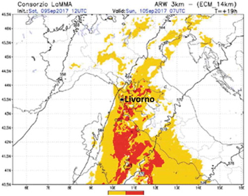
Figure 2. WRF nested domains used for the simulations

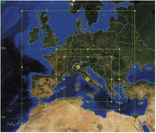
Figure 3. First row: S1 derived soil moisture; second and third rows: six layers SM maps used as WRF input

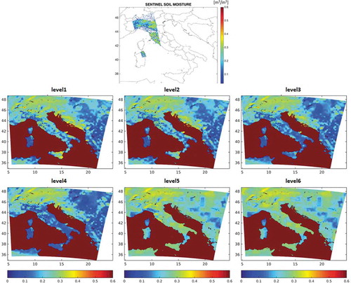
Figure 4. Results of the comparison between reference and WRF-derived cumulated rain rate for the Livorno event obtained using the MODE tool. CENTR_DIST, ANG_DIFF and AREA_RATIO are considered. Left panels: THR ≥48 mm; right panels: THR≥72 mm. Blue bars: control run; red bars: ingestion/assimilation of: LST (1st row), SM (2nd row), SST (3rd row), WS and WD (4th row), ZTD using a GNSS observation every minute; green bar (last row): assimilation of ZTD using only the GNSS observation temporally closest to the assimilation time (last row). The dark blue lines indicate the perfect scores (0 for CENTR_DIST and ANG_DIFF, 1 for AREA_RATIO).

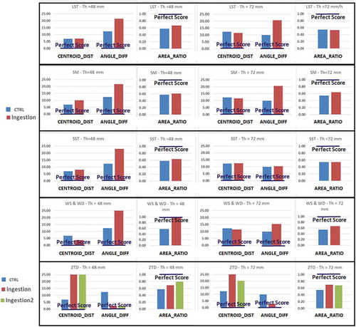
Figure 5. Same as Figure 4, but considering FBIAS (perfect score: 1), PODY (perfect score: 1) and FAR (perfect score: 0)

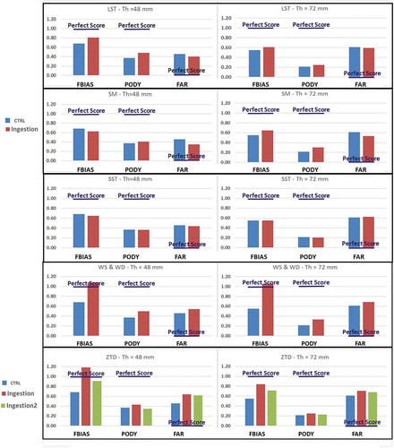
Figure 6. Wind field estimated from the Sentinel-1 observation performed on September 8, 2018 at 17:40 UTC and included in the OWI level-2 product

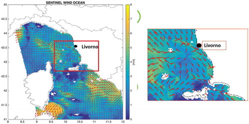
Figure 7. 3D simulated structure composed by rainwater (cyan), graupel (yellow) and snow (grey) microphysics species respectively for the CTRL run (a) and the run with the assimilation of the wind field (c); the horizontal 10m wind intensity represented by red vectors. The red line in panels a and c indicates the location of the vertical section of the two structures to investigate the reflectivity values in the middle of the observed convective structure reported in panels b (for CTRL) and d (for WIND)

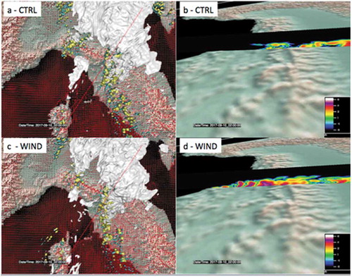
Figure 8. Same as Figure 4 (upper panel) and Figure 5 (lower panel), but considering the combined ingestion of WS and WD, ZTD using a GNSS observation every minute and SM (red bars); green bars: best results obtained with the ingestion of a single variable.

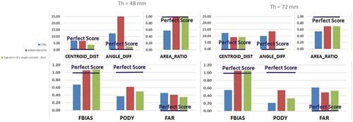
Figure 9. Panel a: Tuscany region hydro-meteorological alert areas; panel b: areas of interest (S3 in green and A6 in red) for this event; panels c and d: hourly mean rainfall over the S3 and A6 alert areas, respectively, comparing the observed rainfall (OBS), the CTRL run, the WIND+SM+ZTD run and a control simulation initialized at 00 UTC on September 9, 2017 (CTRL_00UTC).

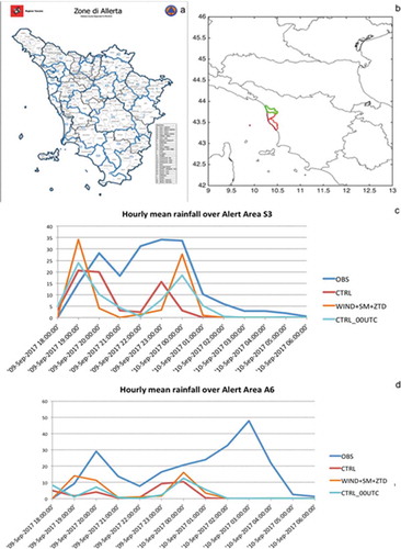
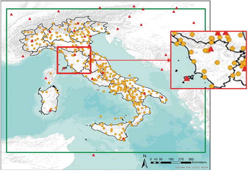
Figure 10. GNSS and EPN (European Permanent Network) stations used in this work with zoom on the stations placed in Tuscany

Available data

For the Livorno event, S1 and S3 data acquired between the afternoon of September 8 and the evening of 9 September 2017 were available. In particular, the following data were directly available through the Sentinel catalogues: 1) LST and SST derived from the Sea and Land Surface Temperature Radiometer (SLSTR) onboard S3, generated on a 1 × 1 km² grid; 2) wind vector (W_S and W_D at 10 m asl) included in the Ocean Wind Field (OWI) component of the Sentinel 1 Level-2 Ocean (OCN) product (again generated on a 1 × 1 km² grid). More specifically, for SST, the Sentinel 3 data acquired on 9 September 2017 at 20:36 UTC were gathered, while for LST, the Sentinel 3 data acquired on 9 September 2017 at 09:50 UTC were used. For what concerns SM, W_D and W_S, S1 observed the Livorno area on 8 September 2017 at 17:14 UTC. To derive SM from S1 data and IWV from GNSS data we relied on retrieval algorithms (described in the Variables retrieval section).

WRF model setup and data assimilation methods

The WRF model (Skamarock et al., 2008) was selected as the numerical weather model to accomplish all the experiments carried out within the framework of the STEAM project. It is a compressible non-hydrostatic model that was developed at the National Center for Atmospheric Research (NCAR) in collaboration with several institutes and universities for operational weather forecasting and atmospheric science research. For this work, WRF version 3.8.1 was adopted. Three domains with two-way nesting setup (Figure 2) were used, at 13.5 (250 × 250 horizontal grid points), 4.5 (451 × 450) and 1.5 km (943 × 883) spatial resolution, with 50 vertical levels (all domains top reached 50 hPa). The selected WRF model setup was based on previous results for this kind of events (Fiori et al., 2014, 2017; Lagasio, Parodi, Procopio, Rachidi, & Fiori, 2017). The two inner domains (4.5 and 1.5 km) allow solving explicitly many convective processes (Kain et al., 2008; Kain, Weiss, Levit, Baldwin, & Bright, 2006) so an explicit treatment of convection is chosen. As for the 13.5 km domain, a parameterization scheme closest to the one used in the GFS global model is chosen (Han & Pan, 2011)

Concerning the surface layer, the MM5 scheme was adopted; this scheme uses stability functions from Dyer and Hicks (1970), Paulson (1970), Webb (1970) to compute surface exchange coefficients for heat, moisture, and momentum. A convective velocity following Beljaars (1995) was used to enhance surface fluxes of heat and moisture. The Rapid Update Cycle (RUC) was chosen for land processes; the scheme has a multi-level soil model with higher resolution in the upper soil layer (0, 5, 20, 40, 160, 300 cm is default). The planetary boundary layer (PBL) scheme is based on the diagnostic non-local Yonsei University PBL (Hong, Noh, & Dudhia, 2006) scheme, as the next generation of the Medium-Range Forecast (MRF) PBL, also using the countergradient terms to represent fluxes due to non-local gradients. As for the microphysics, the WRF single-moment 6-class (WSM6) scheme was used; it extends the WSM5 scheme to include graupel and its associated processes. Of the three WSM schemes, the WSM6 scheme is the most suitable for cloud-resolving grids, considering the efficiency and theoretical backgrounds (Hong & Lim, 2006). Finally, the radiative processes were parameterized by means of the longwave and shortwave Rapid Radiative Transfer Model (RRTMG) schemes (Iacono et al., 2008). The initial and lateral boundary conditions were derived from NCEP-GFS (National Centers for Environmental Prediction Global Forecast System) analysis and forecast data available at a horizontal resolution of 0.25°× 0.25° and a time resolution of 3 h.

The data ingestion was performed according to three different methodologies: direct insertion, a nudging-like technique, and finally a 3DVAR assimilation. Direct insertion is meant hereafter as the substitution of a given variable in the NWM fields with the corresponding one retrieved by EO sensors; it was applied for SST and LST. The nudging-like technique was applied for the SM observations; it included different steps. Firstly, a difference map between the S1-derived SM (reprojected to the WRF grid) and the WRF SM from the first level of soil model (in correspondence with the points observed by S1) was produced; then the resulting map was interpolated to fill the gaps in the S1-derived maps and added to the original WRF SM field in the first (superficial) level. Finally, the new SM field was propagated in the underlying vertical levels by a vertical profile correction through the linear interpolation of the difference between the observed and simulated SM assuming a difference equal to 0 in the deepest level (the S1 observation is only superficial, in the deepest layers the value of the model is more reliable). Figure 3 shows the SM maps resulting from the procedures described above. It can be noted that in the lowest layer there is no influence of the satellite observation and that this influence increases in the upper layers.

W_S and W_D from Sentnel-1 and GNSS were assimilated using the 3 DVAR technique. In particular, for GNSS a 3-h cycle technique was implemented (to take advantage of the high temporal resolution). The 3DVAR main purpose is to provide an optimal estimate of the current status of equation (1) (Ide, Courtier, Ghil, & Lorenc, 1997).

(1) $J(x)=\frac{1}{2}{\left(x-x^b\right)}^T{B}^{-1}\left(x-x^b\right)+\frac{1}{2}{\left(y-y^0\right)}^T{R}^{-1}\left(y-y^0\right)$(1)

where x is the analysis to be found that minimizes the cost function J(x), x^b is the first guess of the NWP model, y° is the assimilated observation, and y= H(x) is the model-derived observation transformed from the analysis x by the observation operator H for comparison against y°. The solution of (1) represents a posteriori maximum likelihood (minimum variance) estimate of the true state given two sources of data: the first guess x^b and the observation y°. The analysis fit to this data is weighted by estimates of their errors B and R, which denote the background error covariance matrix and the observation error covariance matrix, respectively.

The version 3.9.1 of the Data Assimilation system built within the WRF (WRFDA) was chosen. The Control Variable option 5 (CV5) of the WRFDA package was used for the B matrix calculation using the National Meteorological Center (NMC) method (Wang et al., 2014). The NMC method was applied over the entire month of October 2013 with a 24-h lead time for the forecasts starting at 00:00 UTC and a 12-h lead time for the ones initialized at 12:00 UTC of the same day. The differences between the two forecasts (t+ 24 and t+ 12) valid for the same reference time were used to calculate the domains specific error statistics.

The R matrix was assumed to be diagonal, as done in most of the models (Bouttier & Courtier, 1999). Thus, observation error correlations are often assumed to be zero, considering distinct measurements affected by physically independent errors. Conversely, observation error variances are assumed equal to the instrumental errors, thus varying between different variables.

Validation method

To validate the model output for each experiment the Method for Object-Based Diagnostic Evaluation (MODE) tool (Davis, Brown, Bullock, & Halley-Gotway, 2009) was used. Simply speaking, MODE is a basic algorithm for image segmentation and object matching, specifically developed for meteorological applications. After the identification of the objects in the precipitation maps (observed and forecasted), MODE assigns to the object a series of attributes defined both geometrically (e.g. size, orientation) and based on the precipitation values inside the objects. Then, to summarize the performance of forecasts, it compares the attributes between matched forecasted and observed objects. The use of this validation method is mainly due to the fact that when comparing high-resolution observational data analysis and cloud-resolving meteorological forecast, especially in case of deep moist convective and highly localized phenomena, the traditional verification methods suffer from the so-called “double penalty” issue and hence alone cannot provide a measure of spatial and temporal match between the forecast and observed meteorological patterns. In this respect, it is then preferable to take advantage of features based verification technique, such as MODE. For sake of clarity and conciseness, the MODE evaluation in terms of pairs of objects attributes is hereafter summarized using three representative output indices: centroid distance, angle difference and area ratio (Table 3).

Table 3. Description of the MODE-derived spatial indices used in this work.

Index	Description
Centroid Distance	Centroid Distance: Provides a quantitative sense of spatial displacement of forecast (Best score 0).
Angle Difference	For non-circular objects, gives measure of orientation errors (Best score 0)
Area Ratio	Provides an objective measure of whether there is an over- or under-prediction of areal extent of forecast (Best score 1).

Among the different parameters, MODE provides also some classical statistical scores. Then to assess the performance of the forecasts also the probability of detection (PODY), the false alarm ratio (FAR) and the frequency bias (FBIAS) were chosen. These parameters were derived from a contingency table that shows the frequency of “yes” and “no” rain forecasts and occurrences. The four combinations of forecasts (yes or no) and observations (yes or no) are: 1) hit: rain forecasted and actually occurring; 2) miss: rain not forecasted and actually occurring; 3) false alarm: rain forecasted and actually not occurring; 4) correct negative: rain not forecasted and actually not occurring.

PODY is given by the number of hits divided by the total number of observed rainy events:

(2) $PODY=\frac{\mathrm{h}\mathrm{i}\mathrm{t}\mathrm{s}}{\mathrm{h}\mathrm{i}\mathrm{t}\mathrm{s}+\mathrm{m}\mathrm{i}\mathrm{s}\mathrm{s}\mathrm{e}\mathrm{s}}\left(\mathrm{p}\mathrm{e}\mathrm{r}\mathrm{f}\mathrm{e}\mathrm{c}\mathrm{t}\mathrm{s}\mathrm{c}\mathrm{o}\mathrm{r}\mathrm{e}=1\right)$(2)

FAR is given by the number of false alarms divided by the total number of forecasted rainy events:

(3) $FAR=\frac{\mathrm{f}\mathrm{a}\mathrm{l}\mathrm{s}\mathrm{e}\mathrm{a}\mathrm{l}\mathrm{a}\mathrm{r}\mathrm{m}\mathrm{s}}{\mathrm{h}\mathrm{i}\mathrm{t}\mathrm{s}+\mathrm{f}\mathrm{a}\mathrm{l}\mathrm{s}\mathrm{e}\mathrm{a}\mathrm{l}\mathrm{r}\mathrm{m}\mathrm{s}}\left(\mathrm{p}\mathrm{e}\mathrm{r}\mathrm{f}\mathrm{e}\mathrm{c}\mathrm{t}\mathrm{s}\mathrm{c}\mathrm{o}\mathrm{r}\mathrm{e}=0\right)$(3)

FBIAS is given by the total number of forecasted rainy events divided by the total number of observed rainy events:

(4) $FBIAS=\frac{\mathrm{h}\mathrm{i}\mathrm{t}\mathrm{s}+\mathrm{f}\mathrm{a}\mathrm{l}\mathrm{s}\mathrm{e}\mathrm{a}\mathrm{l}\mathrm{a}\mathrm{r}\mathrm{m}\mathrm{s}}{\mathrm{h}\mathrm{i}\mathrm{t}\mathrm{s}+\mathrm{m}\mathrm{i}\mathrm{s}\mathrm{s}\mathrm{e}\mathrm{s}}\left(\mathrm{p}\mathrm{e}\mathrm{r}\mathrm{f}\mathrm{e}\mathrm{c}\mathrm{t}\mathrm{s}\mathrm{c}\mathrm{o}\mathrm{r}\mathrm{e}=1\right)$(4)

Variables retrieval

As previously pointed out, SST and LST were directly available as Sentinel-3 (S3) level-2 products (currently through the Sentinel-3 Pre-Operations Data Hub), while W_S and W_D were directly available as S1 level-2 products (through the Copernicus Open Access Hub). Hence, for these variables, there was no need to use a retrieval algorithm. Conversely, SM and IWV had to be retrieved. As for the latter variable, the quantity that can be estimated from satellite data is the Zenith Total Delay (ZTD) from GNSS and the Slant Total Delay (STD) from S1 using the InSAR technique. ZTD represents the delay induced by the troposphere on GNSS signals in the zenith direction, while STD is the difference between the slant range atmospheric delays of the master and the slave images of an Interferometric pair. Since it was found that, for the Livorno event, there was little water vapour in the atmosphere at the S1 acquisition time, only GNSS-derived ZTD were considered in this study. The methods used to retrieve SM and ZTD are briefly described hereafter.

Soil moisture retrieval from sentinel-1 data

The algorithm developed to estimate SM was conceived to combine a multi-temporal approach with a good computational efficiency. The latter characteristic is particularly suitable for an operational application, such as the use of SM maps in NWP models. A multi-temporal approach to estimate SM from SAR assumes that the temporal scale of variation of soil roughness is considerably slower than that of SM. Hence, if a dense time-series of SAR data is available, as expected using S1, short-term changes in the backscattering coefficient σ° (that represents the SAR measurement) are basically related to SM variations. (Balenzano, Mattia, Satalino, & Davidson, 2011; Kim et al., 2012; Pierdicca, Pulvirenti, & Bignami, 2010).

The algorithm is based on a multi-temporal maximum likelihood (ML) approach (e.g. Kim et al., 2012) used to invert a direct scattering model of backscattering from a bare soil, namely that proposed by Oh (2004). The Oh Model relates the state of the soil, described by the pair (SM,s), where s denotes the height standard deviation of the rough surface, to the backscattering coefficient σ°. This relationship is represented in the form of lookup table (LUT) (Kim et al., 2012; Pierdicca, Pulvirenti, Bignami, & Ticconi, 2013; Pierdicca et al., 2014), which was generated by applying the Oh model considering as inputs 50 values of s (between 0.5 e 4.5 cm with a discretization of 0.0816 cm), 100 values of SM (between 0.05 e 0.4 m³/m³ with a discretization of 0.0035 m³/m³) and 13 values of incidence angle θ (between 26° and 50° with a discretization of 2°). The range of SM and s values is approximately the same used by Pierdicca et al. (2013), (2014) and accounts for the range of validity of the Oh model. As for the θ range, with respect to the S1 Interferometric Wide Swath (IWS) acquisition mode nominal incidence angle range, a larger interval was considered for the LUT to account for topography. For each pair (SM, s), 13 values of σ° at VV polarization (one for each θ value) were computed (indicated as ${\sigma }_{\mathrm{V}\mathrm{V},\mathrm{m}\mathrm{o}\mathrm{d}\mathrm{e}\mathrm{l}}^0$). Note that VV is the default co-polarized channel of S1.

The retrieval algorithm assumes that a time series of M+ 1 measurements (at the current time t and at M previous times t− 1, …, t − M) is available. It performs a least square search minimizing the square difference between measured and modelled values of σ°:

(5) $\begin{array}{rl}& d[SM(t),SM(t-1),...,SM(t-M),s,\theta ]\\ & ={\left\{{\sigma }_{VV,soil}^0(t){|}_{dB}-{\sigma }_{VV,m\mathrm{o}\mathrm{d}\mathrm{e}\mathrm{l}}^0[SM(t),s,\theta ]{|}_{dB}\right\}}^2\\ & +{\left\{{\sigma }_{VV,soil}^0(t-1){|}_{dB}-{\sigma }_{VV,m\mathrm{o}\mathrm{d}\mathrm{e}\mathrm{l}}^0[SM(t-1),s,\theta ]{|}_{dB}\right\}}^2\\ & +......+{\left\{{\sigma }_{VV,soil}^0(t-M){|}_{dB}-{\sigma }_{VV,m\mathrm{o}\mathrm{d}\mathrm{e}\mathrm{l}}^0[SM(t-M),s,\theta ]{|}_{dB}\right\}}^2\end{array}$(5)

where d is the cost function that has to be minimized and the symbol $|{\hspace{0.17em}}_{dB}$ indicates that the backscatter values are expressed in logarithmic units. In (5), ${\sigma }_{\mathrm{V}\mathrm{V},\mathrm{s}\mathrm{o}\mathrm{i}\mathrm{l}}^0$ refers to the soil contribution to the S1 measurements, so that, if vegetation is present, its effects on the S1 backscattering measurements must be corrected before determining the cost function d. The choice of M is a compromise between SM estimation accuracy and computational time; M= 4 was chosen as done by Pierdicca et al. (2014).

The correction of the vegetation effects on σ° is a very critical point for any SM retrieval approach. In fact it is usually based on semi-empirical models that may lack generality. For this study, the Water Cloud Model (WCM, Attema & Ulaby, 1978) was used, with the parameters proposed by Bindlish and Barros (2001) for all land uses. In the WCM, the vegetation is simply represented by a “bulk” parameter, such as the vegetation water content W. Previous studies (e.g. Jackson et al., 2004, 1999) have shown that there exists a direct relationships between W and the Normalized Difference Vegetation Index (NDVI), which can be derived from optical data such as, Sentinel-2, Landsat, or MODIS ones. Here the empirical relationship found by Pierdicca et al. (2013) was used (and NDVI data were extracted from the MOD13Q1 MODIS product, see Huete Didan, van Leeuwen, Miura, & Glenn, 2011):

(6) $W=11.92\times NDVI-2.73\left[\mathrm{k}\mathrm{g}/{\mathrm{m}}^2\right]$(6)

Note that if W< 0.25 kg/m², the influence of vegetation on the radar signal is considered as negligible and the S1 backscatter is not corrected (Pierdicca et al., 2013). Instead, if W >5 kg/m² the retrieval of SM is assumed to be totally insensitive to SM, so that pixels are masked in this case.

Zenith total delay retrieval from GNSS data

Water vapour content of the atmosphere low layer (up to about 10 km), known as troposphere or neutral atmosphere, affects GNSS signals by changing their propagation velocities with respect to that of the light in vacuum. A diminished speed results in a larger observed time $\mathrm{\Delta }t$ to cover the satellite-receiver distance, and eventually to a larger satellite-receiver observed distance $S^{obs}c\mathrm{\Delta }t$. The path delay in length (Slant Total Delay – STD) can be therefore defined as follows (here we disregard the ray bending):

(7) $ST{D}_r^s=S^{obs}-S={\int }_s^{\hspace{0.17em}}\left(\frac{c}{v\left(s\right)}-1\right)ds={\int }_s^{\hspace{0.17em}}\left(n\left(s\right)-1\right)ds={10}^{-6}{\int }_s^{\hspace{0.17em}}N\left(s\right)ds$(7)

where s is the actual signal path here considered equal to the straight satellite-receiver line, n is the refraction index and $N{10}^6\left(n-1\right)$ is the refractivity. By assuming a horizontally layered water vapour distribution, one can express such slant delay as a linear function of the delay along the vertical direction, i.e., the ZTD, above each receiver:

(8) $ST{D}_r^s=ZT{D}_{r}mf$(8)

where mf is the known mapping function, that projects the unknown zenith delay onto the satellite-receiver slant path. Most of the modern mapping functions are expressed using a continued fraction in terms of 1/sin(ε) (Marini, 1972), ε being the satellite elevation, truncated after the third term (Niell, 1996):

(9) $mf\left(\epsilon \right)=\frac{1}{sin\left(\epsilon \right)+\frac{a}{sin\left(\epsilon \right)+\frac{b}{sin\left(\epsilon \right)+c}}}$(9)

The $a,b$ and $c$ parameters are usually taken from a global model, the most used being Niell (Niell,1996), GMF (Böhm, Niell, Tregoning, & Schuh, 2006) and VMF (Böhm & Schuh, 2004). The parameters of the VMF (Vienna Mapping Function) are estimated from ECMWF numerical weather model (Kouba, 2008) with a temporal resolution of 6 h and a spatial resolution of 2° in longitude and 2.5° in latitude.

It is worth reminding here that the tropospheric delay (the word delay is usually referred to the extra distance and is expressed in meters) due to water vapour, is just one out of many other systematic errors affecting GNSS observations which are to be accounted for in order to achieve sub-centimetre accuracy positions. Two different strategies are currently used to deal with those systematic effects: one is based on a combination of the observations of two receivers to a satellite pair, allowing for the removal of the common systematic effects, the other models most of the errors and relies on the currently achieved high accuracy of satellites ephemerides (Héroux & Kouba, 2001). This last strategy, known as Precise Point Positioning (PPP) has been adopted for the STEAM experiment.

PPP mainly models each satellite-receiver observed distance as a function of the unknown station coordinates, receiver clock offset, ZTD (a proper combination of dual frequency data, iono-free combination, gets rid of the ionospheric contribution) and the phase ambiguities (Héroux & Kouba, 2001). A lot of effort has been put in the modelling of the systematic effect, nowadays accounted for by all software implementing GNSS data adjustment for high accuracy positioning purposes.

The observations collected by the GNSS station from all the satellites simultaneously in view at a given epoch involve the same ZTD parameter and receiver clock, while the phase ambiguities and the coordinates of a fixed station are common to all the different epochs of a daily session. The parameters can be retrieved by applying either a Kalman filter approach, thus updating their estimates epoch by epoch based on the past observations only, or a joint least squares adjustment of all the session observations. In the STEAM experiment, the free and open source software goGPS (Realini & Reguzzoni, 2013) was adopted. It was developed by GReD srl, implementing a PPP strategy with a multi-epoch joint least squares adjustment of the observations. The processing settings are summarized in Table 4.

Table 4. GPS processing settings.

Satellite elevation cut-off:	7 degrees
ZTD random walk regularization:	0.015 m/$\sqrt{h}$
ZTD gradients random walk regularization:	0.0015 m/$\sqrt{h}$
Geophysical corrections:	IERS 2010 convention
Ambiguity:	Float
Mapping function:	VMF gridded mapping function
Orbits and satellite clocks:	International GNSS Service (IGS) final products

Results and discussion

The experiments

The WRF simulations were started at the synoptic hour temporally closest to the time of the S1 acquisition, i.e., on 8 September 2017 at 18:00 UTC and lasted 48 h (until 10 September 2017 at 18:00 UTC).

To apply the multi-temporal SM retrieval algorithm previously described, not only the S1 data acquired on 8 September 2017, but also those acquired on September 2, August 27, August 21 and 15 August 2017 were used and the ground range detected (GRD) products were chosen. The GRD data were multi-looked (10 × 10), calibrated and geocoded using the 30 m SRTM DEM. All the Sentinel-derived data were resampled and reprojected to a reference WRF grid (that of the inner domain: Geographic Lat/Lon, WGS84, ~1.5 km of pixel size, corresponding to 0.0135°). The nearest neighbour approach was applied for this purpose, except for the SM maps for which a pixel aggregate resampling, which averages all the pixel values that contribute to the output pixel, was adopted.

ZTD time series at 30-s resolution were estimated for all the geodetic permanent stations within the WRF domain providing free raw GNSS observations. For the selected event, the data of 375 stations were available. An accuracy assessment was performed by comparing the GNSS-derived ZTD to the eight Italian radiosounding datasets, yielding a mean difference of 3 mm and a standard deviation of 14.6 mm (a total of 43 radiosonde launches has been considered).

Firstly, the sensitivity of the WRF model to each single variable was analysed, then the ingestion of one variable at a time was accomplished (besides the control simulation run, as underlined in the Introduction). The values of SM and wind field were assumed as acquired at 18:00 UTC (although S1 acquisition time was 17:40), i.e., at the starting time of the simulations.

S3 derived SST and LST data were ingested into the model via a direct insertion, as previously pointed out. For this purpose, the WRF simulation was stopped at the acquisition time of each variable and then restarted after having replaced the WRF derived variable with the S3 derived one in a warm restart mode. Concerning GNSS-derived ZTD, it was assimilated in WRF using the 3DVAR technique. In particular, the assimilation was cyclically performed every 3 h (throughout the 48h-simulation) in two different ways: 1) considering either a GNSS observation every minute (in a 30-min time window centred at the analysis time), 2) considering only the GNSS observation temporally closest to the analysis time. The assimilation configuration for each experiment is summarized in Table 5.

Table 5. Experiment setup summary.

Experiment	Assimilation timing	Assimilation methods
LST	10 UTC 09/10/2017	Direct Insertion
SST	21 UTC 09/10/2017	Direct Insertion
SM	18 UTC 08/10/2017	Nudging-like
WIND	18 UTC 08/10/2017	3dvar
ZTD3h	3 hour cycling starting at 18 UTC 08/10/2017	3h cycling 3dvar considering GNSS observation every minute in a 30 minutes time window centered at the analysis time
ZTD3h_1ist	3 hour cycling starting at 18 UTC 08/10/2017	3h cycling 3dvar considering GNSS observation temporally closest to the analysis time
WIND+SM+ZTD	Assimilation at the acquisition time of SM and WIND with GNSS-ZTD with a 3h cycling 3dvar	3dvar + nudging-like
CTRL	No assimilation	No assimilation

Analysis of the results of the experiments

As validation data, the rain rate measurements provided by the rain gauge network managed by the Italian Department of Civil Protection (DPC) were chosen. It includes more than 5000 rain gauges covering all the Italian territory. The rain rate measurements were spatially interpolated to be compared with the model forecasts. To evaluate the forecast performances, the rain rate cumulated between September 9 at 18:00 UTC and September 10 at 06:00 UTC (time period when most of the rain fell) was considered, as the sub-daily period including the most intense part of the observed flash-flood-producing storm. Two different thresholds on the cumulated rain (THR hereafter) were considered to identify the objects in the forecast and observation maps by using the MODE tool, namely THR ≥48 mm and THR ≥72 mm. Figure 4 and Figure 5 show the values of the scores computed through MODE obtained in the experiments of ingestion of one variable at a time

In terms of pairs of objects indices (Figure 4), an improvement in terms of the centroid distance (CENTR_DIST) with respect to the control run (CTRL) is achieved through the assimilation of SST, SM and the wind field (W_S and W_D) for THR≥72mm (the assimilation of W_S and W_D improves the result for THR>48mm too). Furthermore, the assimilation of ZTD decreases the angle difference (ANGLE_DIFF) for both the thresholds. Finally, almost all the performed simulations show an improvement in terms of AREA_RATIO with respect to CTRL forecast.

Looking at Figure 5, in terms of classical statistical indices, it can be seen that the ingestion of LST implied an improvement of the forecast performances for all the three parameters considered in this analysis (increase of FBIAS and PODY, decrease of FAR). However, this improvement did not turn out to be very significant except for FBIAS and THR of 48 mm. Even the ingestion of SST did not produce significant impacts on the WRF forecasts. As for SM, its ingestion led to an improvement of all the indices except FBIAS for a threshold of 48 mm. It must be underlined that by ingesting SM, the lowest values of FAR were obtained for both the thresholds.

The most positive impact on the forecast performances was obtained by assimilating the wind field (W_S and W_D). In this case, despite of a slight increase of FAR, a FBIAS close to the perfect score (1, see Figure 5) was obtained and also PODY improved with respect to the CTRL. Furthermore, in terms of rainfall pattern location, the assimilation of the wind field-produced improvements in terms of CENTR_DIST and AREA_RATIO for both the THR (Figure 4). In this case, the role of high-resolution observation assimilation seems to be very important. In fact, the assimilation of high-resolution wind field correcting the original WRF wind field at initialization time that was forced by the low resolution (~25 km) GFS data allowed the model to evolve more in agreement with the physics of the observed convective system. Figure 6 shows the wind field extracted from the S1 OWI level-2 product (8 September 2018–17:40 UTC).

The high-resolution observation assimilation at the initialization time helped the forecast because quantitative precipitation NWP models predictive ability challenges can derive from the poor knowledge of the initial state of the atmosphere at small scales leading to an inevitable model spin-up that often results in an inaccurate simulation of the convective system in terms of timing, location and intensity (Sugimoto, Crook, Sun, Xiao, & Barker, 2009). Thus, the capability to capture small-scale phenomenon is likely the reason of the good impact of the S1-derived wind field on the forecast, even though these data were assimilated more than 24 h before the onset of the event. Usually the data assimilation impacts more the first 12 h; however, this is not the first time in literature that for some modelling and assimilation setup the impact of observations assimilation lasts more than 12 h. Koizumi, Ishikawa, and Tsuyuki (2005) found a positive impact of rain assimilation on the precipitation up to 18 h; Dash, Sahu, and Sahu (2013) found out that in a set of experiments, 3DVAR improvements in simulation can be significant up to 24 h and that the impact of assimilation is visible up to 72-h simulation, although with less magnitude. In this case, the choice of the domain setup (two-way nested with outer domains boundary very far from the inner one and updated every 3 h) could help the assimilation impacts to last more than the usual time range.

To further investigate the impact of wind field assimilation at the model initialization, a reference time step at 02UTC on 10 September 2017, corresponding to the most intense phase of the observed event, was considered. Then, using the VAPOR (Visualization and Analysis Platform for Ocean, Atmosphere, and Solar Researchers, www.vapor.ucar.edu) software, the atmospheric flow field was analysed compared to the CTRL experiment (Figure 7). 3D isosurfaces (5 × 10⁻⁵ kg/kg) for the rainwater, snow and graupel variables have been rendered in combination with the wind field at 10 m in case of the CTRL run (panel a) and the WRF run with the assimilation of the wind field (panel c) at the same time instant (02 UTC of 10 September). By inspecting the 10-min horizontal wind field, it is possible to argue that the assimilation of the S-1 derived wind field (Figure 6) contributed to improve, in comparison to the control run, the persistence and intensity of the convergence responsible for the triggering of the observed highly-precipitating back-building Mesoscale Convective System (MCS). Consequently, the prediction obtained by assimilating the wind field was definitely more in agreement with the physics of the observed MCS. Furthermore, while reflectivity is nearly absent nearby the Tuscany coastlines (Livorno area) for the OL experiment (panel b), conversely stronger activity is apparent in panel b over the Livorno area and downshear the main convective system.

From Figure 4 and Figure 5, it can be deduced that the assimilation of the ZTD derived from a GNSS observation every minute (ZTD3h red bars in the last row of the figures) and that of the ZTD obtained using only the GNSS observation temporally closest to the analysis time (ZTD3h_1ist, green bars) gave rise to quite similar results. A significant improvement of FBIAS was achieved with both forecasts, although associated with a slight increase of FAR (slightly lower in the ZTD3h_1ist simulation). PODY slightly improved with respect to the control simulation (CTRL) only for the ZTD3h simulation. In terms of spatial pattern location, the CENTROID_ DIST evidences a worsening in the rainfall location with respect to CTRL simulation, but big improvements were achieved in terms of AREA_RATIO and ANGLE_DIFF of the convective structure.

From the previous analysis, it emerges that the WRF forecasts showed a large sensitivity to the assimilation of the wind field and water vapour. For both the thresholds used to identify objects through the MODE tool, the assimilation of the wind field produced the best performances for FBIAS, PODY and AREA_RATIO, the assimilation of ZTD produced the best results for ANGLE_DIFF, while the best performances for what concerns FAR were obtained by initializing the WRF run with the S1-derived SM, as previously pointed out. Hence, a further experiment was carried out performing the combined assimilation of the wind field and the ZTD (derived from a GNSS observation closest to the analysis time) in a WRF run initialized with the S1-derived SM. This experiment will be synthetically denoted as WIND+SM+ZTD hereafter. The results are shown in Figure 8, where the scores obtained in this experiment are compared with those obtained in the CTRL run, as previously done, as well as with the best scores (e.g., highest FBIAS and PODY and lowest FAR, CENTROID_DIST and ANGLE_DIFF) obtained in the previous experiments of ingestion/assimilation of one variable at a time. It can be seen that this experiment of combined assimilation of WIND, ZTD and SM enabled to improve the performances obtained in the previous experiments except for the FAR for a THR of 48 mm and the ANGLE DIFF. Overall, the WIND+SM+ZTD experiment produced better results with respect to the experiments of ingestion of a single variable.

In view of an operational forecasting framework, hourly rainfall forecast produced by the WIND+SM+ZTD experiment and the CTRL simulation were compared with the corresponding hourly observed data. To pave the way to this analysis, it is worth to notice that the Italian Civil Protection Department manages the hydro-meteorological warning in terms of alert areas. The Tuscany region is divided into 26 Alert Areas (Figure 9, panel a), but for this event, only two areas were largely affected (A6 and S3 highlighted in Figure 9, panel b). The hourly rainfall obtained for these areas is shown in panels c and d of Figure 9. In case of the S3 area, the WIND+SM+ZTD simulation produced an improvement in terms of rainfall peaks (e.g., underestimation of the second peak is reduced from about 20 mm to about 7 mm) with respect to the CTRL simulation (panel c), while the improvement is less pronounced over the A6 area (panel d). More specifically, concerning the A6 area, the WIND+SM+ZTD simulation enabled a quantitative precipitation forecast (QPF) improvement for the first rainfall peak, but without succeeding in mitigating the underestimation of the second peak. Thus, despite the cyclic update of the forecast every 3 h with ZTD observations, the forecast is not able to fully capture the convective system dynamic. This can be due to the initialization time far from the event and to the GNSS network not particularly dense over the Tuscany region (see Figure 10), then not able to steer the simulated event, triggered over the sea area, towards the A6 area.

It is worth noting that the Italian Civil Protection (and regionals civil protection departments) alert system is based on a daily bulletin issued each day before 13 UTC reporting the forecasted situation for the following 36 h for each Alert Area of each Region (see Figure 9, panel A for the Tuscany region). In this context, it is important to consider that the 18 UTC GFS global model is available at 21.45 UTC and the forecast runtime is 2h30, so that the forecast forced by the 18 UTC GFS is available at 00:15/00:30 UTC. Along the same lines, the forecast initialized with 00 UTC GFS is available at 6:30 UTC. In an operational framework only these two initializations are relevant for issuing the daily alert bulletin, while subsequent initializations at 06 UTC and 12 UTC (available, respectively, at about 12.30 and 20.30 UTC) can be used only for an alert update in a nowcasting framework. Then, to gain a further insight in the effect of the ingestion of the EO-derived products, the lower panels of Figure 10 include also the hourly mean rainfall for a new CTRL run started at 00UTC on 9 September 2017, i.e., close to the event onset (CTRL_00UTC hereafter).

It can be seen that even the CTRL_00UTC was not able to fully capture the observed rainfall peaks and their timing, over the target areas S3 and A6. Moreover, the WIND+SM+ZTD ingestion setup followed more closely the CTRL_00UTC simulation than the CTRL one. Finally, and more importantly, the WIND+SM+ZTD ingestion setup produced higher rainfall peaks with respect to the CTRL_00UTC simulation, especially over the S3 area. Hence, the WIND+SM+ZTD experiment resulted into a win-win situation being able to provide a better QPF over the target Alert Areas even in advance with respect to one that would have been available by forcing WRF with a more recent GFS model instance.

Conclusions

The assimilation of Sentinel-derived products into numerical weather prediction models was rarely attempted so far and can be considered as a challenging problem related to the improvement of the quality of the predictions of high-resolution numerical weather models. In the framework of the STEAM project, a number of experiments was accomplished, making reference to a disastrous flood occurred in Italy in 2017, to verify the effect of the ingestion of surface soil moisture, wind speed and direction, land and sea surface temperature, as well as precipitable water vapour in the WRF model. The work has been performed trying to answer to the ESA investigation about the value added obtained from the synergic use of Sentinel-derived observation and NWP models.

By analyzing a set of sensitivity experiments considering one variable at a time, the most positive impact on the WRF forecasts was achieved by assimilating the wind speed and direction included in the Ocean Wind Field component of the Sentinel-1 Level-2 Ocean product. This finding is likely related to the fact that the triggering of the considered event is strictly due to the presence of a convergence line over the sea area in front of Livorno city. Thus, the assimilation of a high spatial resolution wind field observation over the sea area allowed the model dynamic to evolve in a way more similar to the observed convective event with respect to the CTRL simulation. The assimilation of GNSS-derived zenith total delay turned out to have a positive impact as well, except for an increase of the false alarm rate. For the latter parameter, a decrease was obtained by ingesting the Sentinel-1-derived SM. The ingestion of LST produced a slight improvement of the quality of the WRF predictions, while SST did not show any positive influence on the forecasts.

It must be underlined that the results of the assimilation of the GNSS-derived ZTD are promising even for the assimilation of high-resolution water vapour maps derived from atmospheric phase screen maps generated by applying the interferometric technique to Sentinel-1 data. This application was not carried out in this study, because of the very low values of the water vapour in the atmosphere at the time of the Sentinel-1 observation of the area of interest.

A further improvement of the accuracy of the forecasts was achieved through a combined ingestion of W_S and W_D, ZTD and SM. LST was not considered in this experiment, despite its positive impact on the WRF simulations, because, when high impact weather events occur, cloud cover often hampers the retrieval of this variable.

The outcomes of this study seem to confirm the usefulness of the synergy between high-resolution numerical weather models and a set of Earth Observation products at least for the forecast of high impact weather events. Nonetheless, further investigations are required and will be accomplished in the framework of the STEAM project. Firstly, more than one case study has to be considered, although high-resolution numerical weather predictions are very expensive from a computational point of view. Secondly, an assessment of the value added assimilating high-resolution water vapour maps derived from atmospheric phase screen maps generated by applying the interferometric technique to Sentinel-1 data will be investigated in different cases to see the impact of higher spatial resolution ZTD observations.

Disclosure statement

No potential conflict of interest was reported by the authors.

Additional information

Funding

This work was supported by the European Space Agency [4000121670/17/NL/AF].

References

- Attema, E.P.W., & Ulaby, F.T. (1978). Vegetation modeled as a water cloud. Radio Science, 13(2), 357–364. doi:10.1029/RS013i002p00357
- Balenzano, A., Mattia, F., Satalino, G., & Davidson, M.W.J. (2011). Dense temporal series of C- and L-band SAR data for soil moisture retrieval over agricultural crops. IEEE Journal of Selected Topics in Applied Earth Observations and Remote Sensing, 4(2), 439–450. doi:10.1109/JSTARS.2010.2052916
- Balenzano, A., Satalino, G., Lovergine, F., Rinaldi, M., Iacobellis, V., Mastronardi, N., & Mattia, F. (2013). On the use of temporal series of L- and X-band SAR data for soil moisture retrieval. Capitanata plain case study. European Journal of Remote Sensing, 46(1), 721–737. doi:10.5721/EuJRS20134643
- Beljaars, A.C.M. (1995). The parametrization of surface fluxes in large‐scale models under free convection. Quarterly Journal of the Royal Meteorological Society. doi:10.1002/qj.49712152203
- Bevis, M., Businger, S., Chiswell, S., Herring, T.A., Anthes, R.A., Rocken, C., & Ware, R.H. (1994). GPS Meteorology: Mapping zenith wet delays onto precipitable water. Journal of Applied Meteorology. doi:10.1175/1520-0450(1994)033<0379:GMMZWD>2.0.CO;2
- Bindlish, R., & Barros, A.P. (2001). Parameterization of vegetation backscatter in radar-based, soil moisture estimation. Remote Sensing of Environment, 76(1), 130–137. doi:10.1016/S0034-4257(00)00200-5
- Böhm, J., & Schuh, H. (2004). Vienna mapping functions in vlbi analyses. Geophysical Research Letters, 31(1).
- Böhm, J., Niell, A., Tregoning, P., & Schuh, H. (2006). Global mapping function (gmf): a new empirical mapping function based on numerical weather model data. Geophysical Research Letters, 33(7).
- Bouttier, F., & Courtier, P. (1999). Data assimilation concepts and methods March 1999. Meteorological Training Course Lecture Series. doi:10.1029/2007GL030733
- Cardoso, R.M., Soares, P.M.M., Miranda, P.M.A., & Belo-Pereira, M. (2013). WRF high resolution simulation of Iberian mean and extreme precipitation climate. International Journal of Climatology, 33(11), 2591–2608. doi:10.1002/joc.3616
- Dash, S.K., Sahu, D.K., & Sahu, S.C. (2013). Impact of AWS observations in WRF-3DVAR data assimilation system: A case study on abnormal warming condition in Odisha. Natural Hazards. doi:10.1007/s11069-012-0393-0
- Davis, C.A., Brown, B.G., Bullock, R., & Halley-Gotway, J. (2009). The Method for Object-Based Diagnostic Evaluation (MODE) applied to numerical forecasts from the 2005 NSSL/SPC Spring Program. Weather and Forecasting, 24(5), 1252–1267. doi:10.1175/2009WAF2222241.1
- Dyer, A.J., & Hicks, B.B. (1970). Flux‐gradient relationships in the constant flux layer. Quarterly Journal of the Royal Meteorological Society. doi:10.1002/qj.49709641012
- El Hajj, M., Baghdadi, N., Zribi, M., Belaud, G., Cheviron, B., Courault, D., & Charron, F. (2016). Remote sensing of environment soil moisture retrieval over irrigated grassland using X-band SAR data. Remote Sensing of Environment, 176, 202–218. doi:10.1016/j.rse.2016.01.027
- Fiori, E., Comellas, A., Molini, L., Rebora, N., Siccardi, F., Gochis, D.J., … Parodi, A. (2014). Analysis and hindcast simulations of an extreme rainfall event in the Mediterranean area: The Genoa 2011 case. Atmospheric Research. doi:10.1016/j.atmosres.2013.10.007
- Fiori, E., Ferraris, L., Molini, L., Siccardi, F., Kranzlmueller, D., & Parodi, A. (2017). Triggering and evolution of a deep convective system in the Mediterranean Sea: Modelling and observations at a very fine scale. Quarterly Journal of the Royal Meteorological Society. doi:10.1002/qj.2977
- Hajnsek, I., Jagdhuber, T., Member, S., Schön, H., Papathanassiou, K.P., & Member, S. (2009). Potential of estimating soil moisture under vegetation cover by means of PolSAR. IEEE Transactions on Geoscience and Remote Sensing, 47(2), 442–454. doi:10.1109/TGRS.2008.2009642
- Han, J., & Pan, H.-L. (2011). Revision of convection and vertical diffusion schemes in the NCEP global forecast system. Weather and Forecasting. doi:10.1175/waf-d-10-05038
- Heroux, P., Kouba, J., Collins, P., & Lahaye, F. (2001). Gps carrier-phase point positioning with precise orbit products. In Proceedings of the KIS (pp. 5-8).
- Hong, S.-Y., & Lim, J.-O.J. (2006). The WRF single-moment 6-class microphysics scheme (WSM6). Journal of the Korean Meteorological Society, 43(2), 129–151.
- Hong, S.-Y., Noh, Y., & Dudhia, J. (2006). A New Vertical Diffusion Package with an Explicit Treatment of Entrainment Processes. Monthly Weather Review. doi:10.1175/mwr3199.1
- Hornacek, M., Wagner, W., Sabel, D., Truong, H.-L., Snoeij, P., Hahmann, T., … Doubkova, M. (2012). Potential for high resolution systematic global surface soil moisture retrieval via change detection using Sentinel-1. IEEE Journal of Selected Topics in Applied Earth Observations and Remote Sensing, 5(4), 1303–1311. doi:10.1109/JSTARS.2012.2190136
- Huete, A., Didan, K., van Leeuwen, W., Miura, T., & Glenn, E. (2011). MODIS vegetation indices. In Remote Sensing and Digital Image Processing, 11, 579–602. doi:10.1007/978-1-4419-6749-7_26
- Iacono, M.J., Delamere, J.S., Mlawer, E.J., Shephard, M.W., Clough, S.A., & Collins, W.D. (2008). Radiative forcing by long-lived greenhouse gases: Calculations with the AER radiative transfer models. Journal of Geophysical Research Atmospheres. doi:10.1029/2008JD009944
- Ide, K., Courtier, P., Ghil, M., & Lorenc, A. (1997). Unified notation for data assimilation: Operational, sequential and variational. Journal of the Meteorological Society of Japan. doi:10.5194/npg-18-49-2011
- Iriza, A., Dumitrache, R.C., Lupascu, A., & Stefan, S. (2016). Studies regarding the quality of numerical weather forecasts of the WRF model integrated at high-resolutions for the Romanian territory. Atmosfera, 29(1), 11–21. doi:10.20937/ATM.2016.29.01.02
- Jackson, T.J., Chen, D., Cosh, M., Li, F., Anderson, M., Walthall, C., … Hunt, E.R. (2004). Vegetation water content mapping using Landsat data derived normalized difference water index for corn and soybeans. Remote Sensing of Environment, 92(4), 475–482. doi:10.1016/j.rse.2003.10.021
- Jackson, T.J., Le Vine, D.M., Hsu, A.Y., Oldak, A., Starks, P.J., Swift, C.T., … Haken, M. (1999). Soil moisture mapping at regional scales using microwave radiometry: The Southern Great plains hydrology experiment. Geoscience and Remote Sensing, IEEE Transactions On, 37(5), 2136–2151. doi:10.1109/36.789610
- Kain, J.S., Weiss, S.J., Bright, D.R., Baldwin, M.E., Levit, J.J., Carbin, G.W., … Thomas, K.W. (2008). Some practical considerations regarding horizontal resolution in the first generation of operational convection-allowing NWP. Weather and Forecasting. doi:10.1175/2008waf2007106.1
- Kain, J.S., Weiss, S.J., Levit, J.J., Baldwin, M.E., & Bright, D.R. (2006). Examination of convection-allowing configurations of the WRF model for the prediction of severe convective weather: The SPC/NSSL spring program 2004. Weather and Forecasting. doi:10.1175/waf906.1
- Kim, S.B., Tsang, L., Johnson, J.T., Huang, S., Van Zyl, J.J., & Njoku, E.G. (2012). Soil moisture retrieval using time-series radar observations over bare surfaces. IEEE Transactions on Geoscience and Remote Sensing, 50(5 PART 2), 1853–1863. doi:10.1109/TGRS.2011.2169454
- Koizumi, K., Ishikawa, Y., & Tsuyuki, T. (2005). Assimilation of precipitation data to the JMA mesoscale model with a four-dimensional variational method and its impact on precipitation forecasts. SOLA. doi:10.2151/sola.2005-013
- Kouba, J. (2008). Implementation and testing of the gridded vienna mapping function 1 (vmf1). Journal Of Geodesy, 82(4–5), 193-205.
- Lagasio, M., Parodi, A., Procopio, R., Rachidi, F., & Fiori, E. (2017). Lightning potential index performances in multimicrophysical cloud-resolving simulations of a back-building mesoscale convective system: The Genoa 2014 event. Journal of Geophysical Research. doi:10.1002/2016JD026115
- Marini, J. W. (1972). Correction of satellite tracking data for an arbitrary tropospheric profile. Radio Science, 7(2),223-231.
- Mateus, P., Catalao, J., & Nico, G. (2017). Sentinel-1 Interferometric SAR mapping of precipitable water vapor over a country-spanning area. IEEE Transactions on Geoscience and Remote Sensing, 55(5), 2993–2999. doi:10.1109/TGRS.2017.2658342
- Mateus, P., Miranda, P.M.A., Nico, G., Catalão, J., Pinto, P., & Tomé, R. (2018). Assimilating InSAR maps of water vapor to improve heavy rainfall forecasts: A case study with two successive storms. Journal of Geophysical Research: Atmospheres, 123(7), 3341–3355. doi:10.1002/2017JD027472
- Mateus, P., Tomé, R., Nico, G., Member, S., & Catalão, J. (2016). Three-dimensional variational assimilation of InSAR PWV using the WRFDA model. IEEE Transactions on Geoscience and Remote Sensing, 54(12), 7323-7330. doi:10.1109/TGRS.2016.2599219
- Niell, A. E. (1996). Global mapping functions for the atmosphere delay at radio wavelengths. Journal of Geophysical Research: Solid Earth, 101(B2), 3227-3246.
- Oh, Y. (2004). Quantitative retrieval of soil moisture content and surface roughness from multipolarized radar observations of bare soil surfaces. IEEE Transactions on Geoscience and Remote Sensing, 42(3), 596–601. doi:10.1109/TGRS.2003.821065
- Panegrossi, G., Ferretti, R., Pulvirenti, L., & Pierdicca, N. (2011). Impact of ASAR soil moisture data on the MM5 precipitation forecast for the Tanaro flood event of April 2009. Natural Hazards and Earth System Science, 11(12), 3135–3149. doi:10.5194/nhess-11-3135-2011
- Paulson, C.A. (1970). The mathematical representation of wind speed and temperature profiles in the unstable atmospheric surface layer. Journal of Applied Meteorology. doi:10.1175/1520-0450(1970)009<0857:TMROWS>2.0.CO;2
- Pichelli, E., Ferretti, R., Cimini, D., Panegrossi, G., Perissin, D., Pierdicca, N., … Rommen, B. (2015). InSAR water vapor data assimilation into mesoscale model MM5: Technique and pilot study. IEEE Journal of Selected Topics in Applied Earth Observations and Remote Sensing, 8(8), 3859–3875. doi:10.1109/JSTARS.2014.2357685
- Pierdicca, N., Pulvirenti, L., & Bignami, C. (2010). Soil moisture estimation over vegetated terrains using multitemporal remote sensing data. Remote Sensing of Environment, 114(2), 440–448. doi:10.1016/j.rse.2009.10.001
- Pierdicca, N., Pulvirenti, L., Bignami, C., & Ticconi, F. (2013). Monitoring soil moisture in an agricultural test site using SAR data: Design and test of a pre-operational procedure. IEEE Journal of Selected Topics in Applied Earth Observations and Remote Sensing, 6(3), 1199–1210. doi:10.1109/JSTARS.2012.2237162
- Pierdicca, N., Pulvirenti, L., & Pace, G. (2014). A prototype software package to retrieve soil moisture from sentinel-1 data by using a bayesian multitemporal algorithm. IEEE Journal of Selected Topics in Applied Earth Observations and Remote Sensing, 7(1), 153–166. doi:10.1109/JSTARS.2013.2257698
- Realini, E., & Reguzzoni, M. (2013). Gogps: open source software for enhancing the accuracy of low-cost receivers by single-frequency relative kinematic positioning. Measurement Science and Technology, 24(11), 115010.
- Schepanski, K., Knippertz, P., Fiedler, S., Timouk, F., & Demarty, J. (2015). The sensitivity of nocturnal low-level jets and near-surface winds over the Sahel to model resolution, initial conditions and boundary-layer set-up. Quarterly Journal of the Royal Meteorological Society, 141(689), 1442–1456. doi:10.1002/qj.2453
- Skamarock, W.C., Klemp, J.B., Dudhi, J., Gill, D.O., Barker, D.M., Duda, M.G., … Powers, J.G. (2008). A description of the advanced research WRF Version 3. Technical Report, (June), 113. doi:10.5065/D6DZ069T
- Sugimoto, S., Crook, N.A., Sun, J., Xiao, Q., & Barker, D.M. (2009). An examination of WRF 3DVAR radar data assimilation on its capability in retrieving unobserved variables and forecasting precipitation through observing system simulation experiments. Monthly Weather Review. doi:10.1175/2009mwr2839.1
- Wang, H., Huang, X.Y., Sun, J., Xu, D., Zhang, M., Fan, S., & Zhong, J. (2014). Inhomogeneous background error modeling for WRF-var using the NMC method. Journal of Applied Meteorology and Climatology. doi:10.1175/JAMC-D-13-0281.1
- Webb, E.K. (1970). Profile relationships: The log‐linear range, and extension to strong stability. Quarterly Journal of the Royal Meteorological Society. doi:10.1002/qj.49709640708