High-resolution mapping of protected agriculture in Mexico, through remote sensing data cloud geoprocessing

ABSTRACT

In recent years, plasticulture, which is broadly defined as the use of plastics in agriculture, including greenhouse, tunnels and plastic mulch has become a fast-growing production system. While in the 1970s, the system was used on 2.8 M ha worldwide, the area had grown to 38 M ha in 1996/97 and is still increasing at a rapid rate: In Asia and Africa, the use of plastic greenhouses is growing by 15-30% per year. Therefore, plasticulture is expected to rise in many agrarian countries such as Mexico. Nonetheless, there are negative effects of plasticulture, that need to be correctly addressed in order to have responsible rural landscape management. Ergo our study attempts, through cloud geoprocessing of Sentinel-2 imagery, to rapidly provide a reliable and updated high-resolution map of protected agriculture that employs plastics (mostly tunnels and greenhouses). This map can be used as a basis for a protected agriculture monitoring system in Mexico, and eventually help to effectively plan the upcoming rural development, e.g. by providing input for territorial planning, showing the municipal rural practice trends, and monitoring the markets and its economic impacts.

KEYWORDS:

• Protected agriculture
• plasticulture
• remote sensing
• Google Earth Engine
• Sentinel 2

Introduction

Human population is increasing as well as the demand for food and agricultural products, which is expected to grow by 70–100% of the total production of 2010 by 2050 (Godfray et al., 2010). In the context of globalization, many countries, such as Mexico, are reorienting their agriculture towards exports. To achieve these goals, global annual agricultural expansion and improvements in production technology are expected (Tilman, Balzer, Hill, & Befort, 2011).

One of the most common technologies is Protected Agriculture (PA) which consists of infrastructure that modifies the natural environment, to protect the crops from external factors and enhance growth (Jensen & Malter, 1995). These include mulching, controlled environment agriculture, hydroponics, greenhouses, tunnels, etc. In this work, we focused solely on PA that employs plastics (mostly tunnels and greenhouses).

PA has shown to be a reliable option for agriculture, is productive, conservative of water and nutrients, suitable for automatization and easy to implement (Jensen & Malter, 1995). It also increases yields of crops, improves quality, and decreases the incidence of pathogens (Demchak, 2009; Lamont, 2009). These advantages have made PA rise worldwide, even in desertic areas. For instance, it is estimated that plastic-mulched land cover grows to an annual rate of 20% globally (Lu, Di, & Ye, 2014). Therefore, plasticulture can play an important role to satisfy the growing farm products’ demand by increasing food production (Lamont, 2009)

In Mexico, the PA has been incentivized. The subsidies destinated to PA projects reached near 2000 million Mexican pesos (≈ 103,715,000 USD) of the federal budget between 2001 and 2007 (IMAT, 2015). This has resulted in an exponential growth of the total area of PA in Mexico, starting with 100 ha in 1970 and reaching 25,000 ha by 2016 (Bastida Tapia, 2017). Most areas of PA are found in the central and North-western parts of Mexico (states of Sinaloa, Jalisco, Michoacán and Baja California) (SIAP, 2015).

However, PA has negative effects on various environmental aspects and at different scales. It can modify microclimates, alter distributions of pollinators, and create aesthetic pollution of the rural landscape (Jensen & Malter, 1995; Picuno, Tortora, & Capobianco, 2011). Additionally, due to their low production cost, plastics are in high demand in agriculture. They are also largely discarded which is a huge contribution to the plastic waste problem (Jambeck et al., 2015) due to their extremely low biodegradation rate (Meneses, Corrales, & Valencia, 2007; Sanders, Granberry, & Cook, 1996). In addition, PA presents an organic waste disposal problem, because all the roots, leaves and steams that do not represent the final harvest are thrown away (Tolón Becerra & Lastra Bravo, 2010). Also, it requires specialized equipment that means the greater cost to the farmers (Sanders et al., 1996). It has been shown that PA uses around three times more agro-chemicals than non-plastic-protected practices, which increases toxicity, runoff and soil erosion in the surrounding areas (Arnold, Luckenbach, & Unger, 2004; Vázquez, Pardo, Suso, & Quemada, 2006; Wan & El-Swaify, 1999). Similarly, these technologies in many cases need more water because it increases the internal temperature that entails higher evaporation rates, which leads to the use of low-quality water and excessive underground water extraction (Tolón Becerra & Lastra Bravo, 2010). Therefore, as PA has both positive and negative impacts, it is imperative to develop a monitoring system that allows measurement of changes in PA, so the effects of this practice can be properly addressed, leading towards responsible planning of rural landscapes.

Consequently, around the world, there has been a growing interest towards a reliable mapping and detection of plasticulture (Yang et al., 2017). Some of those efforts concentrate in remote sensing using satellite and hyperspectral data, because it offers the advantage that it covers much larger areas, than other techniques along with high accuracy mapping and fast processing. Remote sensing data have been used to map plasticulture in many parts of the world such as: Weifang District (Yang et al., 2017), Xiaoshan District (Wu, Deng, Wang, Ma, & Tahmassebi, 2016) and Xinjiang province (Lu et al., 2014) all in China, Southern Italy (Picuno et al., 2011), Israel (Levin, Lugassi, Ramon, Braun, & Ben-Dor, 2007) and Almeria in Spain (Agüera, Aguilar, & Aguilar, 2006; Aguilar, Nemmaoui, Novelli, Aguilar, & Lorca, 2016; Novelli, Aguilar, Nemmaoui, Aguilar, & Tarantino, 2016), using various remote sensing data as, for example, Landsat 5–8, QuickBird, Sentinel-2 imagery and hyperspectral AISA-ES photography.

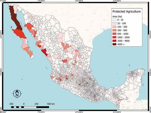
In Mexico, there have been very few attempts to map and monitor plasticulture. The official data from the Agroalimentary and Fisheries Information Service (Servicio de Información Agroalimentaria y Pesquera, SIAP) is the only available source for plasticulture at a national scale (SIAP, 2015) (Figure 1). Even so, these data merely show the area of plasticulture per municipality, without mapping the infrastructures. Considering the rapid increase of plasticulture in the country, the updating of these data is far too slow to take effective action concerning landscape management, territorial growth planning, inspection or rapid response (Gorelick et al., 2017; Shimabukuro et al., 2011).

Figure 1. Protected agriculture in Mexico, number of hectares (ha) per municipality for the entire country. Own elaboration based on the data from SIAP (2015)

This study aimed at mapping, in near real time, the current plasticulture infrastructure (august 2017- august 2018) over the entire Mexican territory using Google Earth Engine (GEE), a relatively new software that enables big data analysis (Gorelick et al., 2017).

Materials and methods

We used the available highest resolution free access data, in order to implement a near real-time monitoring system that can be easily replicated and improved.

Material

We obtained Sentinel-2 multispectral imagery, acquired from august 2017 to august 2018, with less than 5% cloud percentage, through the GEE dataset catalogue. These images contain 13 spectral bands representing top of the atmosphere (TOA) reflectance (level 1-C), and an additional band for cloud mask information. Spatial resolution is 10, 20 or 60 m, depending on the spectral band, and revisiting interval is 5 days (European Space Agency, 2015).

We also used ancillary data: [1] a digital elevation model (DEM) at 30 m resolution, provided by the Shuttle Radar Topography Mission (SRTM) (Farr et al., 2007), [2] the night-time data from the Visible Infra-red Imaging Radiometer Suite (VIIRS) Day/Night Band (DNB) for the whole year (Aug. 2017- Aug. 2018) (Mills, Weiss, & Liang, 2013), [3] a digital map (shapefile) of the urban boundaries of localities with more than 15,000 inhabitants from the National Housing Commission (CONAVI, 2017), [4] a digital map of the Mexican physiographic provinces (National Institute of Statistics and Geography (INEGI) 2001), [5] the statistics on per municipality plasticulture area (SIAP 2015) and [6] a land cover/land use map, scale 1/250,000 from INEGI (2012).

Methods

We used the information on the cloud band (QA60) to mask cirrus and opaque clouds. The images were stacked, computing the median value of all of them for each band. We choose the median instead of average in order to avoid noise due to outlier values. As a following step, eight indexes, some of them developed to enhance plastic cover, were calculated a 10-m resolution (Table 1).

Table 1. Description of the computed indexes using Sentinel-2 band information. The abbreviations refer to the spectral bands: NIR near-infrared, SWIR short wave infrared, RED, GREEN and BLUE are the bands in the visible parts of the spectrum

Index	Abbreviation	Description	References
Normalized Difference Vegetation Index	(NDVI)	$\frac{NIR-RED}{NIR+RED}$	(Rouse, Haas, & Deering, 1974)
Normalize Difference Build-up Index	(NDBI)	$\frac{SWIR1-NIR}{SWIR1+NIR}$	(Zha, Gao, & Ni, 2003)
Normalized Difference Water Index	(NDWI)	$\frac{GREEN-NIR}{GREEN+NIR}$	(McFeeters, 1996)
Green Normalized Difference Vegetation Index	(GNDVI)	$\frac{NIR-GREEN}{NIR+GREEN}$	(Gitelson, Kaufman, & Merzlyak, 1982)
Plastic Greenhouses Index	(PGI)	$\left\{\begin{array}{cc}0& whenNDVI>0.73\\ 100\ast & \left(\frac{BLUE\ast \left(NIR-RED\right)}{1-mean\left(BLUE+GREEN+NIR\right)}\right)\\ 0& whenNDBI>0.005\end{array}\right.$	(Yang et al., 2017)
Plastic-mulched landcover index	(PMLI)	$\frac{SWIR1-RED}{SWIR1+RED}$	(Lu et al., 2014)
Normalized Difference SWIR2_NIR	(SW2_N)	$\frac{SWIR2-NIR}{SWIR2+NIR}$	(Aguilar et al., 2016)
Normalized Difference SWIR1+ SWIR2_NIR	(SW1+ SW2_N)	$\frac{\left(\frac{SWIR1+SWIR2}{2}\right)-NIR}{\left(\frac{SWIR1+SWIR2}{2}\right)+NIR}$	(Aguilar et al., 2016)

Ancillary data were used to mask areas where plasticulture is unlike to occur. For instance, as extensive plasticulture does not occur on steep areas, a mask was created for areas with a slope above 8% (Ortho Books, 2001). In the same manner, plasticulture is primordially a rural activity (Jensen & Malter, 1995), the Monthly average radiance composite images from the VIIRS nighttime data were summed to produce a one-year “night-light accumulation” layer, which was thresholded at 59 nanoWatts/cm²/sr to create an urban mask. This mask was complemented using the urban boundaries from the CONAVI digital map.

We choose the maximum entropy classifier (Mann, Mcdonald, Mohri, Silberman, & Walker, 2009) over all the other classifiers in GEE, because it enables performing a classification for only two classes (protected agriculture or not) and gives a map of probability ranging, which should be thresholded to obtain a binary final classification. This classifier is widely used in species distribution modelling using georeferenced localities for the presence and pseudo absence of the targeted species (Phillips, Anderson, & Schapire, 2006). The choice of the threshold applied to the probabilities enables users to control the trade-off between omission and commission errors. The classification was carried out using a stratified strategy. Each one of the 15 physiographic provinces was classified independently in order to reduce the diversity of land covers and reduce spectral confusion.

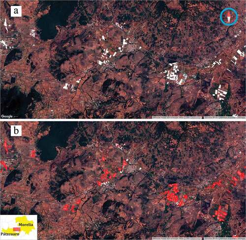
First, we made an attempt to classify a small region between the cities of Morelia and Pátzcuaro, in the State of Michoacán, one of the states where a large amount of PA is reported. We delimited training polygons through visual interpretation of the Sentinel colour composite and Google Earth imagery with the closest temporal match possible (Figure 2). A water mask (NDWI > 0) and a plastic mask with the PGI only considering classifying pixels with similar spectral behavior to plastics films of PA were created. In order to determine the optimum bands combination to accurately map plasticulture, we employed the transformed divergence index (Swain, 1973). This separability index, based on the assumption of normality, uses the mean and variance-covariance matrices of data representing two classes to assess their separability. As GEE does not allow to carry out this analysis, it was necessary to download the Sentinel composite image. Afterwards, we performed a non-supervised classification to produce training data for the non-plasticulture land cover classes able to represent the spectral variability of these classes. The global separability index was focused on the separability of PA versus any other land cover category by weighing higher separability indices involving PA.

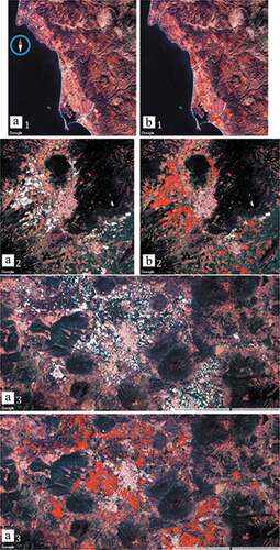
Figure 2. Plasticulture in the region between Patzcuaro and Morelia cities, as shown in the bottom left box, both panels display the composite one-year Sentinel-2 image. (a) Bare composite image, the bright white pixels are the plastic films of PA infrastructures. (b) highlighted in red are shown the areas that were detected as PA by our classifier (these vectors are not the ones made by visual interpretation)

After bands selection, we carried out a binary classification (PA/all other non-PA covers) for the Pátzcuaro region using as training data for PA and non-PA, 1000 and 5000 randomly selected pixels, respectively, inside and outside the PA polygons previously visually identified. Finally, we executed the classifier, resulting in an accurate mapping and detection of plasticulture.

After mapping PA in the Pátzcuaro region, we carried out the classification for the entire physiographic Pátzcuaro belongs to. To do so we employ a different training data set by including 5000 random points for non PA covers. A similar procedure was then applied to the other physiographic provinces.

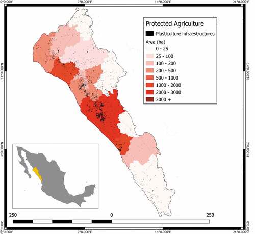
Then, we compared the PA national map to the Sentinel colour composite and Google Earth imagery, evaluating every municipality with a more than 25 ha difference against the SIAP data, and manually cleaned by eliminating commission and drawing omission polygons. The final result (a sample is depicted in Figure 3) was a binary map with PA and non-PA covers.

Figure 3. Protected Agriculture in the State of Sinaloa, according to this study. Location of all plasticulture infrastructures on the national territory, and number of hectares per municipality

Accuracy assessment

The accuracy assessment was carried out following Olofsson, Foody, Stehman, and Woodcock (2013); Olofsson et al. (2014). These authors indicated a strategy to assess accuracy and estimate areas of maps which present rare class(es). Therefore, we used a stratified random sampling, and the sample size (N) was determined using equation (1)(1) $N={\left(\frac{\sum W_i\ast U_i}{S\left(\text{^}O\right)}\right)}^2$(1) .

(1) $N={\left(\frac{\sum W_i\ast U_i}{S\left(\text{^}O\right)}\right)}^2$(1)

where N is the number of samples, S(Ô) the standard error of the estimated overall accuracy that we would like to achieve, W_i is the mapped proportion of area of the category i, and U_i the expected user’s accuracy of class i (proportion of the area mapped as category i which is truly i).

It is recommended between 50 and 100 samples be assigned to the rare classes and then distribute the remaining samples to the other classes proportionally to the class area. However, in the case of our PA map, the PA class is extremely rare (about 50,000 ha for a total territory of 189,991,000 ha). According to equation (1)(1) $N={\left(\frac{\sum W_i\ast U_i}{S\left(\text{^}O\right)}\right)}^2$(1) , N will depend mainly on the user accuracy of the dominant class (non-PA) which is expected to be very high because the class PA is extremely rare. As a consequence, the size of the sample will not be very large. The 50–100 samples assigned to the PA stratum will allow to assess commission error accurately. However, it is doubtful that the remaining samples can enable the detection of PA omission error. For instance, supposing an omission error of 100,000 ha (twice the size of the reported area by SIAP), the probability that a random sample unit outside the mapped as PA area falls into an omitted PA area is (100,000)/(189,991,000–50,000) = 0.0005. Consequently, the probability (p) that a sample of 500 random sampling units does not detect any omission errors is p^500 = 0.77, this probability with a sample of 1000 units, is still p^1000 = 0.59. Therefore, in the most likely case, the only commission will be evaluated, and omission error will not be detected, leading to the underestimation of the rare class area. Paradoxically, in the very unlikely case that one or more sample units detect an omission error, this would lead to an overestimation of the rare class area when correcting the area estimates using the confusion matrix.

As an attempt to deal with this problem, we constructed an additional stratum, in which most of the omission error is likely to occur. For this purpose, we used a 1 km buffer around all the PA polygons of those municipalities where this cover represents more than 2% of the whole municipality area according to the SIAP data. Selected samples were visually interpreted using both the Sentinel colour composite and Google Earth imagery. We also used formulas for estimating accuracy and areas along with the intervals of confidence of these estimators from Card (1982). Finally, we overlaid the map with a land use/cover map dated 2011 in order to assess the impact of PA on land use/cover change.

Results and discussion

The separability analysis showed that combinations using more than five bands do not significantly increase the separability due to the high correlation between bands and indices. Therefore, we selected the five bands combination which enables the highest separability which includes the Blue, NIR, SWIR1, SWIR2 and SW2_N bands. Classifications were carried out for the different physiographic regions and resulting probability images were thresholded with the value of 0.8. We chose this value in order to favour commission error (easy to detect and to correct using the accuracy assessment) and to reduce, as much as possible, omission errors.

Based on expected user accuracies of 0.7 for PA and 0.95 for non-PA categories, we estimated the sampling size in 476 verification plots. Fifty sample units were assigned to the areas mapped as PA, 50 to the buffer area around the area mapped as PA in municipalities where important PA was reported and the remaining units (376) to the rest of the territory. All the plots were selected randomly.

Then, we elaborated the confusion matrix (Table 2) and calculated the omission and commission error after carrying out the adjustments proposed by Card (1982). Taking into account omission and commission errors depicted in the confusion matrix, we estimated the area of PA estimated in 40,311 ha ± 10,231. However, as we show in the Methods section, omission errors outside the buffer area are unlikely to be detected using only 376 samples. So, if we consider that the buffer stratum did not enable us to take into account the totality of the omission errors, then the PA area estimate is likely underestimated. Another aspect is the large confidence interval around the area estimate. In order to reduce this uncertainty, the sample size for the PA and Buffer strata should be increased. However, using 100 samples for these two strata instead of 50 will likely reduce the confidence interval to 7,200 ha only.

Table 2. Raw confusion matrix

	PA	Non-PA (Buffer)	Non-PA (Outside buffer)
Total Area (ha)	47,584	151,273	189,990,788	Total plots	Commission Error	User’s Accuracy
PA	36	0	14	50	28%	0.72 ± 0.12
Non-PA (Buffer)	2	48	0	50	0.46%
Non-PA (outside buffer)	0	0	376	376
Total plots	38	48	390	476
Omission Error	5%	3%
Producer’s Accuracy	0.85 ± 0.17					Overall: 96.64%

Accuracy assessment and area estimates of such maps with both rare and large classes is not an easy task because the omission error of the rare class is difficult to evaluate. As an attempt to overcome this issue, we used a stratified strategy using a stratum where omission error is expected. In the present case, the stratum enables us to detect and evaluate omission error and therefore, after correcting the estimates through the confusion matrix. Without this stratified strategy, the area of PA would have been likely underestimated. However, it is possible that the used stratum was not able to “concentrate” enough the omission error of PA and that some amount of omission error was not taken into account. Other strategies can be envisaged to construct the strata. The first one can be based on the Maximum Entropy classification probability values. As cells with a probability above 0.8 were classified as PA, cells in which probability belongs to an interval between a certain threshold and 0.8 were not classified as PA but present a certain spectral affinity to PA and, therefore, may be prone to be misclassified. Another approach can be based on spatial modelling: maps of suitability for PA can be elaborated using explanatory variables and PA mapped areas (Camacho Olmedo, Paegelow, Mas, & Escobar, 2018; Mas, Kolb, Paegelow, Camacho Olmedo, & Houet, 2014) and areas with high suitability used as strata.

To contrast our results with the data reported by SIAP, we subtracted our municipal PA area estimations from both sources (Figure 4). We found that Michoacán, instead of Sinaloa, is the leading state at PA area; similarly, of the total 2458 municipalities nationwide, 57 had differences (either commission or omission) of 100 ha or more, meaning that both studies give very similar or equal area estimations for most of the municipalities. Figure 5 allows to compare the image and the obtained map in three of the municipalities with most PA area.

Figure 4. Frequency Histogram of the differences between estimates. The X axis is the difference between SIAP and ours municipal PA area estimations in ha while the Y axis is the frequency in the logarithmic scale. Most municipalities have a difference of less than 100 ha, and differences of more than 400 ha are very rare

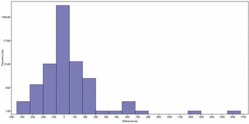
Figure 5. Plasticulture Infrastructure in different windows of three municipalities with a large PA area. All windows contain two panels: A and B; panel A contains the Sentinel colour composite, where the plasticulture infrastructure is easily discernible, panel B contains the same composite image as background, and an additional layer in bright red which shows the polygons classified as PA. The windows correspond to the following municipalities: 1) Ensenada, Baja California State; 2) Zapotlan, Jalisco; and 3) Zamora, Michoacan

Nonetheless, from those 57 discrepant municipalities, according to our study 32 of them had a less estimated area (omission) and 25 had a greater estimated area (commission) against the SIAP data. Most of these omissions happened in the North of the country, for example, in the municipalities of Elota and Navolato, both in Sinaloa, with “missing” areas of 1676 ha and 1274 ha, respectively, or Mulegue and Ensenada in Baja California (589 ha and 583 ha, respectively). However, an additional examination did not allow to find unclassified PA areas. Probably, due to the arid conditions of these regions, PA is temporal, which leads to a failure in properly detecting these areas using the annual composite image. Although it is possible that PA has decreased, it is unlikely due to increasing global and national trends. Another omission example was Villa Guerrero in the State of Mexico (central region), this municipality is the major producer of flowers in Mexico and presents the singularity of having the PA infrastructures within the urban area. In this case, the missing 762 ha was considered as urban area.

Commissions, on the other hand, occurred mostly in the central region of the country, being Michoacán and Guanajuato the states with more area over-estimated by the present study in comparison with the SIAP data, with 3819 and 1416 additional ha, respectively. No particularly important commission errors were detected in these areas and the observed area differences can be explained by the rapidly increasing PA area in central Mexico, and thus the difference between studies can be attributed to the updating of the present study (2018 imagery) in comparison with SIAP (2015).

In Mexico, PA is mostly concentrated on several areas which need to be monitored to properly manage plasticulture down effects. The overlaying procedure between our maps of PA and a land use/cover map dated 2011, showed that 93% of the PA was established on croplands, mainly irrigated areas. Therefore, almost all PA establishes on areas already with an agricultural use and occur as a shift of agricultural activities. A deep analysis of PA distribution would allow to develop a projection under prospective scenarios.

Concluding remarks

Knowing the scope that can be achieved with GEE and the goals behind its development (Kumar & Mutanga, 2018), we hope that this work can set an antecedent towards a national accurate PA monitoring system and, ultimately, contribute to understanding rural changes and the promotion of sustainable rural management.

This study is, as far as we know, the first attempt to map plasticulture infrastructures and PA at a national level using cloud geoprocessing. The maps we obtained present an acceptable accuracy and show a consistency, with the approximations of the tendencies for Mexico, and the SIAP data. Our approach can be improved in the future, for instance by using Bottom Of the Atmosphere (BOA) imagery, employing more accurate training data for the classifier, calculating the separability for each physiographic province, experimenting with other classifiers, developing a more suited accuracy assessment, including eventually a phase of ground-truthing.

Geolocation information

The study area involves the entire territory of Mexico.

Acknowledgments

This research was possible thanks to a residency, within the framework of an international cooperation agreement recently settled, between the Environmental Geography Research Centre (CIGA) at the National Autonomous University of Mexico (UNAM), and the Rural and Environmental Studies Faculty (FEAR) at the Pontifical Xavierian University in Bogota, Colombia (PUJ-Bogota) that aims at promoting scientific collaboration between both countries. This study was supported by the project PAPIME (PE301919) “Herramientas para la enseñanza de la Geomática con programas de código abierto” (DGAPA - UNAM). We also thank the careful revision of our manuscript. The final corrections were done during a sabbatical stay of the second author with the support of PASPA-UNAM.

Data availability statement

The corresponding shapefile and metadata produced as a result of this study can be found at http://lae.ciga.unam.mx/recursos/Agricultura_Protegida_2018.rar

Disclosure statement

No potential conflict of interest was reported by the authors.

Additional information

Funding

This work was supported by the PAPIME-DGAPA-UNAM [PE301919].

References

- Agüera, F., Aguilar, M.A., & Aguilar, F.J. (2006). Detecting greenhouse changes from QuickBird imagery on the Mediterranean coast. International Journal of Remote Sensing, 27(21), 4751–4767. doi:10.1080/01431160600702681
- Aguilar, M.A., Nemmaoui, A., Novelli, A., Aguilar, F.J., & Lorca, A.G. (2016). Object-based greenhouse mapping using very high-resolution satellite data and Landsat 8 time series. Remote Sensing, 8(6), 10–12. doi:10.3390/rs8060513
- Arnold, G.L., Luckenbach, M.W., & Unger, M.A. (2004). Runoff from tomato cultivation in the estuarine environment: Biological effects of farm management practices. Journal of Experimental Marine Biology and Ecology, 298(2), 323–346. doi:10.1016/S0022-0981(03)00366-6
- Bastida Tapia, A. (2017). Evolución y Situación Actual de la Agricultura Protegida en México. In Memorias, sexto congreso internacional de investigación de ciencias básicas y agronómicas (pp. 281–294). Texcoco, Edo. De México: Universidad Autónoma Chapingo.
- Camacho Olmedo, M.T., Paegelow, M., Mas, J.-F., & Escobar, F. (Editors). (2018). Geomatic approaches for modeling land change scenarios (pp. 525). New York: Series: Lecture Notes in Geoinformation and Cartography, Springer. Print ISBN 978-3-319-60800-6, Online ISBN 978-3-319-60801-3.
- Card, D. (1982). Using know map category marginal frequencies to improve estimates of thematic map accuracy. Photogrammetry Engineering and Remote Sensing, 48(3), 431–439.
- Comision Nacional de Vivienda (CONAVI). (2017). Mapas con los perimetros de contención urbana (PCU) de las localidades urbanas del Sistema Urbano Nacional. Gobierno de México. Retrieved from https://datos.gob.mx/busca/dataset/mapas-con-los-perimetros-de-contencion-urbana-pcu-de-las-localidades-urbanas/resource/f9c81c39-744c-44b0-bdf5-abe43f65737a
- Demchak, K. (2009). Small fruit production in high tunnels. HortTechnology, 19(1), 44–49. doi:10.21273/HORTSCI.19.1.44
- European Space Agency. (2015). SENTINEL-2 user handbook. Retrieved from https://sentinel.esa.int/web/sentinel/user-guides/sentinel-2-msi
- Farr, T.G., Rosen, P.A., Caro, E., Crippen, R., Duren, R., Hensley, S., … Alsdorf, D. (2007). The shuttle radar topography mission. Reviews of Geophysics, 45(RG2004). doi:10.1029/2005RG000183.1.INTRODUCTION
- Gitelson, A.A., Kaufman, Y.J., & Merzlyak, M.N. (1982). Using known map category marginal frequencies to improve estimates of thematic map accuracy. Remote Sensing of Environment, 58(3), 431–439. doi:10.1016/S0034-4257(96)00072-7
- Godfray, H.C.J., Beddington, J.R., Crute, I.R., Haddad, L., Lawrence, D., Muir, J.F., … Toulmin, C. (2010). Food security: The challenge of feeding 9 billion people. Science, 327(February), 812–819. doi:10.1126/science.1185383
- Gorelick, N., Hancher, M., Dixon, M., Ilyushchenko, S., Thau, D., & Moore, R. (2017). Google Earth Engine: Planetary-scale geospatial analysis for everyone. Remote Sensing of Environment, 202, 18–27. doi:10.1016/j.rse.2017.06.031
- Instituto Mexicano de Tecnologia del Agua (IMAT). (2015). Estudio y Desarrollo De Tecnología Modular Para Una Agricultura Protegida Sustentable. Jiutepec: Morelos.
- Instituto Nacional de Estadística y Geografía (INEGI). (2001). Conjunto de datos vectoriales Fisiográficos. Continuo Nacional serie I. Provincias fisiográficas. Gobierno de México. Retrieved from https://www.inegi.org.mx/app/biblioteca/ficha.html?upc=702825267575
- Instituto Nacional de Estadística y Geografía (INEGI). (2012). Conjunto de datos vectoriales de uso de suelo y vegetación escala 1:250000, serie V. Gobierno de México. Retrieved from http://www.conabio.gob.mx/informacion/metadata/gis/usv250s5ugw.xml?_httpcache=yes&_xsl=/db/metadata/xsl/fgdc_html.xsl&_indent=no
- Jambeck, J.R., Geyer, R., Wilcox, C., Siegler, T.R., Perryman, M., Andrady, A., … Law, K.L. (2015). Plastic waste inputs from land into the ocean. Marine Pollution, 347(6223), 768–771. doi:10.1126/science.1260879
- Jensen, M.H., & Malter, A.J. (1995). Protected agriculture: A global review. Washington, D.C.: World Bank Publications. Retrieved from https://books.google.es/books?hl=es&id=F1eghGKD6bwC&oi=fnd&pg=PR7&dq=advantages+of+protected+agriculture&ots=upA-BvlbiE&sig=FoAYR9l8gv55y425zljbR_XWnRI#v=onepage&q&f=false
- Kumar, L., & Mutanga, O. (2018). Google Earth Engine applications since inception: Usage, trends, and potential. Remote Sensing, 10(10), 1–15. doi:10.3390/rs10101509
- Lamont, W.J.J. (2009). Overview of the use of high tunnels worldwide. HortTechnology, 19(1), 25–29. doi:10.21273/HORTSCI.19.1.25
- Levin, N., Lugassi, R., Ramon, U., Braun, O., & Ben-Dor, E. (2007). Remote sensing as a tool for monitoring plasticulture in agricultural landscapes. International Journal of Remote Sensing, 28(1), 183–202. doi:10.1080/01431160600658156
- Lu, L., Di, L., & Ye, Y. (2014). A decision-tree classifier for extracting transparent plastic-mulched Landcover from Landsat-5 TM images. IEEE Journal of Selected Topics in Applied Earth Observations and Remote Sensing, 7(11), 4548–4558. doi:10.1109/JSTARS.2014.2327226
- Mann, G.S., Mcdonald, R., Mohri, M., Silberman, N., & Walker, D. (2009). Efficient large-scale distributed training of conditional maximum entropy models. Advances in Neural Information Processing Systems, 22, 1231–1239.
- Mas, J.-F., Kolb, M., Paegelow, M., Camacho Olmedo, M.T., & Houet, T. (2014). Inductive pattern-based land use/cover change models: A comparison of four software packages. Environmental Modelling & Software, 51(1), 94–111. doi:10.1016/j.envsoft.2013.09.010
- McFeeters, S.K. (1996). The use of the Normalized Difference Water Index (NDWI) in the delineation of open water features. International Journal of Remote Sensing, 17(7), 1425–1432. doi:10.1080/01431169608948714
- Meneses, J., Corrales, C.M., & Valencia, M. (2007). Síntesis y caracterización de un polímero biodegradable a partir del almidón de Yuca. Revista EIA, 8, 57–67.
- Mills, S., Weiss, S., & Liang, C. (2013). VIIRS day/night band (DNB) stray light characterization and correction. Proc. SPIE, 8866. doi: 10.1117/12.2023107
- Novelli, A., Aguilar, M.A., Nemmaoui, A., Aguilar, F.J., & Tarantino, E. (2016). Performance evaluation of object-based greenhouse detection from Sentinel-2 MSI and Landsat 8 OLI data: A case study from Almería (Spain). International Journal of Applied Earth Observation and Geoinformation, 52, 403–411. doi:10.1016/j.jag.2016.07.011
- Olofsson, P., Foody, G.M., Herold, M., Stehman, S.V., Woodcock, C.E., & Wulder, M.A. (2014). Good practices for estimating area and assessing accuracy of land change. Remote Sensing of Environment, 148, 42–57. doi:10.1016/j.rse.2014.02.015
- Olofsson, P., Foody, G.M., Stehman, S.V., & Woodcock, C.E. (2013). Making better use of accuracy data in land change studies: Estimating accuracy and area and quantifying uncertainty using stratified estimation. Remote Sensing of Environment, 129, 122–131. doi:10.1016/j.rse.2012.10.031
- Ortho Books. (2001). All about greenhouses. Meredith Books, (Ed.), (first edit). Des Moines, Iowa: Meredith Publishing Group. Retrieved from https://books.google.com.co/books?id=OsMq-bzvWyYC&printsec=frontcover&source=gbs_ge_summary_r&cad=0#v=onepage&q&f=false
- Phillips, S.J., Anderson, R.P., & Schapire, R.E. (2006). Maximum entropy modeling of species geographic distributions. Ecological Modelling, 190(3–4), 231–259. doi:10.1016/j.ecolmodel.2005.03.026
- Picuno, P., Tortora, A., & Capobianco, R.L. (2011). Analysis of plasticulture landscapes in Southern Italy through remote sensing and solid modelling techniques. Landscape and Urban Planning, 100(1–2), 45–56. doi:10.1016/j.landurbplan.2010.11.008
- Rouse, W., Haas, H., & Deering, W. (1974). Monitoring vegetation systems in the great plains with ERTS. Proceedings of the Third ERTS Symposium, NASA SP-35 (December). Washington, DC.
- Sanders, D., Granberry, G., & Cook, W.P. (1996). Plasticulture for commercial vegetables. North Carolina State University: NC Cooperative Extension Service. Extension Document, ( AG-489). Retrieved from https://content.ces.ncsu.edu/plasticulture-for-commercial-vegetables#section_heading_5149
- Servicio de Información Agroalimentaria y Pesquera (SIAP). (2015). Superficie cubierta y número de instalaciones de agricultura protegida (2015). Dirección de Soluciones Geoespaciales. Retrieved from http://infosiap.siap.gob.mx/gobmx/datosAbiertos.php
- Shimabukuro, Y.E., Santos, J., Rudorff, B.F.T., Arai, E., Duarte, V., & Lima, A. (2011). Detección operacional de deforestación y de áreas quemadas en tiempo casi real por medio de imágenes del sensor MODIS. In Aplicaciones de sensor MODIS para el monitoreo del territorio (pp. 123–143). México: CIGA-INECC. Retrieved from http://www.ciga.unam.mx/publicaciones/images/abook_file/aplicacionesMODIS.pdf
- Swain, P.H. (1973). Pattern recognition: A basis for remote sensing data analysis. NASA Technical Report, LARS-11157 (January). Retrieved from https://ntrs.nasa.gov/search.jsp?R=19730008457
- Tilman, D., Balzer, C., Hill, J., & Befort, B.L. (2011). Global food demand and the sustainable intensification of agriculture. PNAS, 108(50), 20260–20264. doi:10.1073/pnas.1116437108
- Tolón Becerra, A., & Lastra Bravo, X. (2010). La agricultura intensiva del poniente almeriense. Diagnóstico e instrumentos de gestión ambiental. M+A. Revista Electrónica De Medioambiente, 8, 1.
- Vázquez, N., Pardo, A., Suso, M.L., & Quemada, M. (2006). Drainage and nitrate leaching under processing tomato growth with drip irrigation and plastic mulching. Agriculture, Ecosystems and Environment, 112(4), 313–323. doi:10.1016/j.agee.2005.07.009
- Wan, Y., & El-Swaify, S.A. (1999). Runoff and soil erosion as affected by plastic mulch in a Hawaiian pineapple field. Soil and Tillage Research, 52(1–2), 29–35. doi:10.1016/S0167-1987(99)00055-0
- Wu, C.F., Deng, J.S., Wang, K., Ma, L.G., & Tahmassebi, A.R.S. (2016). Object-based classification approach for greenhouse mapping using Landsat-8 imagery. International Journal of Agricultural and Biological Engineering, 9(1), 79–88. doi:10.3965/j.ijabe.20160901.1414
- Yang, D., Chen, J., Zhou, Y., Chen, X., Chen, X., & Cao, X. (2017). Mapping plastic greenhouse with medium spatial resolution satellite data: Development of a new spectral index. ISPRS Journal of Photogrammetry and Remote Sensing, 128, 47–60. doi:10.1016/j.isprsjprs.2017.03.002
- Zha, Y., Gao, J., & Ni, S. (2003). Use of normalized difference built-up index in automatically mapping urban areas from TM imagery. International Journal of Remote Sensing, 24(3), 583–594. doi:10.1080/01431160304987