Exploring parameter selection for carbon monitoring based on Landsat-8 imagery of the aboveground forest biomass on Mount Tai

1

ABSTRACT

Forests play a fundamental role in stabilizing the global climate. Aboveground biomass (AGB) is important to the global carbon balance and environmental protection. Remotely sensed features such as single-band information, vegetation indices, texture features and terrain factors have been assessed to accurately estimate the forest biomass. A feature selection SVM-RFE (support vector machine recursive feature elimination) method is proposed to explore the relationship between the biomass and parameters derived from the Mount Tai area Landsat-8 imagery, thereby improving the AGB estimation accuracy. The least significant parameter is recursively removed according to a scoring function to determine the optimal subset of parameters. The performance of the SVM-RFE algorithm biomass feature selection method is then compared with the widely used stepwise regression method. The results show that the SVM-RFE method is superior to the stepwise linear regression method. And it could accurately estimate the AGB compared with field measurements in the context of the recent reducing emissions from forest deforestation and degradation (REDD) mechanism adopted by the United Nations.

KEYWORDS:

• Feature selection
• Landsat-8
• SVM-RFE
• forest biomass

Introduction

Forests contain approximately 80% of all global terrestrial aboveground carbon stocks (Baccini, Laporte, Goetz, Sun, & Dong, 2008). The quantification of carbon stocks is important for assessing the role of forests in the global carbon cycle and reducing emissions due to forest deforestation and degradation in developing countries (Andersen, Strunk, Temesgen, Atwood, & Winterberger, 2012) (Barbosa, Melendez-Pastor, Navarro-Pedreño, & Bitencourt, 2014) (Blackard et al., 2008). Redd programme could provide all stakeholders, including local community with benefits (Birigazzi et al., 2019) (Mardiatmoko, Kastanya, & Hatulesila, 2019). Many national survey organizations have developed their own quality declaration guidelines (Tejada, Görgens, Espírito-Santo, Cantinho, & Ometto, 2019) (Uller et al., 2019). As an important indicator of forest growth, biomass has been widely used to evaluate the influence of forest regions on the atmospheric carbon cycle and environmental protection (Fernández-Manso, Fernández-Manso, & Quintano, 2014). Field measurements often provide base data for mapping the forest biomass over a range of scales (Fernández-Manso et al., 2014). However, forest data collection campaigns over large regions are time-consuming and not well suited for detecting changes because a single measurement campaign may extend over several years (Lu, Mausel, Brondízio, & Moran, 2004).

The development of optical sensor data acquisition technology has provided the capability to estimate forest vegetation characteristics. Several studies have determined that bio/geophysical parameters such as aboveground biomass (AGB) affect spectral reflectance in the visible and near-infrared (NIR) wavelengths (Lee, Kook, Shin, Kim, & Kim, 2007). These implicitly assumed relations between biophysical parameters and remotely sensed optical data are commonly used to monitor forest resource dynamics.

The effectiveness of forests as carbon sinks can be estimated using optical remotely sensed data with empirical and physical approaches. Empirical methods relate a measure of reflectance to a variable of interest through a regression equation (Návar, Ríos-Saucedo, Pérez-Verdín, Rodríguez-Flores, & Domínguez-Calleros, 2013) (Fang & Liang, 2005). However, empirical approaches lack flexibility. Forest vegetation reflectance depends on complex interactions among several internal and external factors that may temporally and spatially vary. No universal relationship exists between vegetation and a spectral signature. Therefore, a physically based approach may overcome multiple limitations of these techniques, such as the generality and limited robustness of empirical models (Návar et al., 2013) (Fang & Liang, 2005) (Darvishzadeh, Skidmore, Schlerf, & Atzberger, 2008). Invertible forest reflectance models are widely used physically based models that account for shadowing and multiple scattering effects, which represent major challenges for vegetation index and spectral mixture analyses (Darvishzadeh et al., 2008) (Schlerf & Atzberger, 2006) (Xiao, Liang, Wang, Song, & Wu, 2009). Invertible forest reflectance models are independent of vegetation type and generally applicable to different sites and sampling conditions. However, the model inversion process is time intensive and not always unique (Darvishzadeh et al., 2008) (Schlerf & Atzberger, 2006) (Xiao et al., 2009).

The identification of informative biomass variables is of fundamental and practical importance to AGB estimation (Eckert, 2012) (Foody, Boyd, & Cutler, 2003) (Kelsey & Neff, 2014). The biomass model variables contain spectral information, texture metrics, vegetation indices, topological factors and tasseled cap data. Among these biomass variables, many are irrelevant, redundant and even decrease the estimation accuracy, as some variables are weakly correlated with the AGB or highly correlated with each other. Effective methods are required to identify the most valuable biomass variables and improve estimations of the AGB.

Many algorithms have been proposed to solve the variable selection problem in the fields of medicine and computer vision (Cai, Zhang, & Hao, 2011) (Quinzán, Sotoca, & Pla, 2009) (Shen, Guo, Wu, & Wu, 2011) (Guyon, Weston, Barnhill, & Vapnik, 2002) (Doquire & Verleysen, 2013) (Ghosh, Ramteke, & Srinivasan, 2014). Multivariate statistical process monitoring methods, such as principal component analysis, partial least squares regression, Fisher discriminant analysis and correspondence analysis, are widely used. Various pattern classification-based approaches have also been used to determine optimal variables, including artificial neural network, support vector machine and k-nearest neighbor methods.

Most forest AGB estimation studies have used the multiple linear regressions model to identify the optimal biomass variables based on more than two bands. The biomass estimation potential of optical imagery has been explored using AVNIR-2 data, and significant improvements have been made by establishing texture index ratios for high-dimensionality data (Sarker & Nichol, 2011). Forest biomass variables have been used to predict the AGB using feedforward neural network models. The results of previous studies suggest that models that include image texture variables are more strongly correlated with biomass than models with only physical and spectral variables (Foody et al., 2001). Biomass and carbon estimation models can be developed using multiple linear stepwise regression models. The correlations between these parameters and the stratum-specific plot data have been analyzed using Pearson’s correlation (Sarker & Nichol, 2011). Ensemble methods, such as random forest, have been used to enhance the biomass prediction accuracy (Utanga, Adam, & Cho, 2012).

To the best of our knowledge, however, few studies have investigated the non-parametric variable selection methods, especially the support vector machine recursive feature elimination (SVM-RFE) algorithm, for regression-based remote sensing applications. The SVM-RFE algorithm can recursively remove the least significant parameter via backward elimination, dramatically enhancing the efficiency of feature selection (Qiu, Fu, & Fu, 2013).

The goal of this paper is to investigate the potential of the optimal biomass selection approach using the SVM-RFE algorithm and Landsat-8 imagery from the Mount Tai forest. The results are compared with the commonly adopted stepwise regression method.

This paper is organized as follows. The study area and data are described in Section 2. The approach is explained in Section 3. Section 4 presents the experiments and discusses the results. Section 5 concludes the paper and outlines future work.

Study area and data

Study area

The study area is located on Mount Tai, Shandong Province, China (116° 50′ – 17° 12′ E,36° 11′ – 36° 31′N; Figure 1). Mount Tai was listed on the world cultural and natural heritage site list in 1985. The land cover is mainly forest, which is fragmented by small tourism areas. Mount Tai encompasses ~242 and ranges from 150 m to 1545 m above sea level. The climate is characterized by consistent rainfall throughout the year, with an average annual rainfall of approximately 1088 mm and a mean annual temperature of over 5°C. The prominent tree species in the area include oak, locust, poplar, willow, elm, green ailanthus and pine.

Figure 1. Study area: Mount Tai, Eastern China.

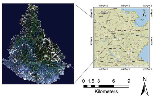
Image data

Landsat-8 was successfully launched from the Vandenberg Air Force Base in California on 11 February 2013. The Landsat-8 satellite carries a two-sensor payload, including the Operational Land Imager (OLI) and the Thermal Infrared Sensor (TIRS), which are summarized in Table 1. Landsat-8 data are acquired in 185 km swaths and segmented into 185 km*180 km scenes, which are defined by path and row coordinates in the second Worldwide Reference System (WRS-2) (Roy et al., 2014) (Ding, Zhao, Zheng, & Jiang, 2014).

Table 1. Landsat-8 bands and wavelengths.

Band description	Wavelength (μm)
Band 1 – Coastal aerosol	0.43–0.45
Band 2 – Blue	0.45–0.51
Band 3 – Green	0.53–0.59
Band 4 – Red	0.64–0.67
Band 5 – Near infrared	0.85–0.88
Band 6 – SWIR 1	1.57–1.65
Band 7 – SWIR 2	2.11–2.29

A Landsat-8 image (WRS-2, Path 122/Row 35) covering the entire study area was acquired on 21 May 2013, with a sun azimuth and sun elevation angle of 127.1° and 66.8°, respectively. The radiance image was atmospherically corrected using the Fast Line-of-Sight Atmospheric Analysis of Spectral Hypercube (FLAASH) algorithm in ENVI 5.1 (Environment for Visualizing Images: ENVI, 2014). The study area includes mountainous terrain, which impacts the optical sensors’ ability to differentiate shaded terrain, affecting the reflectance. An illumination correction (topographic normalization) was performed using the widely used cosine model and a 30 m-resolution digital elevation model (DEM) (Tan, Wolfe, Masek, Gao, & Vermote, 2010) (Tan et al., 2013).

Forest measurement data

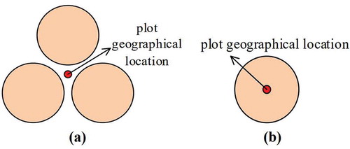
The field campaign was performed from May 13 to 18 May 2013. This period was characterized by high biomass productivity. Random sampling was adopted in this study. The field data were collected at 48 temporary sample plots, which included 5 clustered circular plots (Figure 2(a)) and 42 circular plots (Figure 2(b)). These plots covered the major forest types of Mount Tai. The clustered circular plot was sampled via three sub-plots. Each sub-plot area was as large as 200. The circular plot had an area of 450.

Figure 2. Sample plots: (a) clustered circular plot and (b) circular plot.

The geographical locations of the plots were measured using a non-differential GPS (HOLUX M-241, Holux Technology Inc.) with a positional error of <15 under a canopy. The diameters (DBH: diameter at breast height, 1.30 above the ground) and heights of individual living trees were measured in each plot. Each tree species was also identified. The trees with DBH values less than 5 were not included in the survey. The tree height was measured using a laser range finder (OPTI-LOGIC 400LH, Opti-Logic Corporation). A leveling rod was used for trees shorter than 3 . The DBH was measured at a height of 1.3 using a tape measure.

Methods

An allometric equation was used to calculate the forest AGB based on the forest inventory data. Forest biomass variables such as single-band information, vegetation indices, texture features and terrain factors were extracted from Landsat-8 and used as feature selection model inputs. The performance of the widely used stepwise linear regression model was compared to the proposed SR-SVM-RFE and SVM-RFE algorithms.

Field biomass calculation

Individual tree biomass calculations are commonly based on the species, DBH and height. In our study, the forest-field AGB was calculated from equations based on the allometric equation as follows:

(1)

(2)

where is the aboveground biomass of the individual trees, and are the regression parameters, is the diameter at breast height, is the standard error of the estimation and is the correction factor, which enables the calculations in all of the plots.

The AGB was calculated for each individual tree and then averaged to obtain a plot value for all 48 plots. Subsequently, the AGB results were converted to tons per hectare ().

Forest biomass variable extraction

As shown in Table 2, the forest biomass model variables can be generally divided into four categories: single-band information, vegetation indices, texture features and terrain factors. The simple reflectance values of all eight individual bands [coastal aerosol (COA), blue (B), green (G), red (R), near-infrared (NIR), cirrus and two shortwave infrared (SWIR1, SWIR2) bands] were used to investigate the biomass estimation potential.

Table 2. Landsat-8 remotely sensed features.

Category	Parameters
Single bands	Landsat-8 bands 1–7(B1-B7)
Vegetation indices	NDVI
	SAVI
	AFRI5
	EVI
	ARVI
Texture features	Mean
	Variance
	Homogeneity
	Contrast
	Dissimilarity
	Entropy
	Second moment
	Correlation
Topological factor	Slope
	Aspect

The vegetation index expresses the image values observed in two or more wavebands as a single value that is related to the biophysical variable of interest. Vegetation indices include the normalized difference vegetation index (NDVI), the difference vegetation index (DVI), the ratio vegetation index (RVI), the soil and atmospherically resistant vegetation index (SARVI), the transformed soil atmospherically resistant vegetation index (TSARVI), the multi-vegetation index (MVI) and the perpendicular vegetation index (PVI) (Huete, 1988) (Karnieli, Kaufman, Remer, & Wald, 2001).

Image texture is a measure of variability in pixel values among neighboring pixels within a defined analysis window. The metric is commonly used to identify objects or regions of interest in a given image. Texture has been used to map forest biomass in dense tropical forests and may be a better predictor of biomass than spectral vegetation indices in some regions. Texture variables were derived from Landsat-8 images using grey-level co-occurrence matrix (GLCM) methods. GLCM texture measures were calculated for three different window sizes of 3 × 3 pixels. The entropy, contrast, homogeneity, mean, correlation, variance, dissimilarity, correlation and second moment are the primary textural feature statistical measures.

The terrain factors in this study primarily include the slope and aspect. The terrain factor calculations were based on the grid cell altitude values and the altitude values of direct neighboring cells (typically, the 8 neighboring cells).

SVM-RFE

Redundancy generally exists between different image parameters, preventing forest biomass estimation. Therefore, this study adopted the stepwise linear regression method to initially process the image parameters. Numerical variables should be normalized as before pre-processing. Given a numerical variable Y, the min-max normalization formula is given as

(3)

where is the normalized value of , ranging from . The variables and represent the maximum and minimum value of , respectively.

The algorithm is based on sequential backward elimination feature selection (Qiu et al., 2013) (Li, Zhao, Song, & Yang, 2008) (Mundra, Kumar, Kumar, Jayaraman, & Kulkarni, 2007) (Mundra & Rajapakse, 2010) (Samb, Camara, Ndiaye, Slimani, & Esseghir, 2012) (Zhou & Tuck, 2007), which mainly utilizes the cost function that is trained by SVM to construct the parameter ranking. The lowest-scoring parameters are eliminated until a single parameter remains. The parameter order list is determined in decreasing order of parameter importance.

The procedure is described as follows:

1. Let parameter set s = [1, 2, …, n] and ranked list r =[].

2. Use the parameter set to train the SVM regression and calculate the cost function J.

3. Construct the cost function for all parameters.

4. Find the lowest-scoring parameter from the current parameter set s.

5. Update the ranked list r = [s (f), r] and remove the lowest-scoring parameter from the current parameters set s until only one parameter remains.

The cost function could be written as follows:

(4)

Where represents cost function, represents feature weight.

The flow chart of the SVM-RFE approach is depicted in Figure 3.

Figure 3. Flow chart of the SVM-RFE algorithm.

Experimental results and analysis

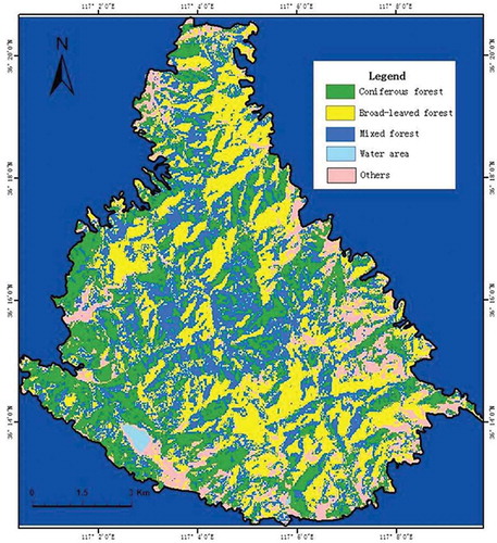
The forest vegetation was classified into coniferous, broadleaf and mixed forest classes based on the Landsat-8 imagery. The biomass estimation models were then established using the stepwise linear regression and SVM-RFE methods for the coniferous, broadleaf and mixed forest species.

Image classification

The Mount Tai Landsat-8 image was classified for biomass estimation using the maximum likelihood classifiers. The forest vegetation was classified into coniferous, broadleaf and mixed forest species classes based on field survey and sample plot data. The results are shown in Figure 4.

Figure 4. Vegetation classification map of the Mount Tai area.

Coniferous forest species estimation

As shown in Table 3, Pearson’s correlation analysis between the coniferous forest species biomass and Landsat-8 image parameters identified one parameter with a significant coefficient. This parameter was the GreenVariance, with r = 0.576 (p = 0.01). Moderate correlations (p = 0.05) were identified for the SWIR1Variance and Slope.

Table 3. Statistically significant Pearson’s correlation coefficients and between the biomass and parameters derived from the Landsat-8 data.

Forest Species	Parameter	Pearson’s r
Coniferous (n = 24)	GreenVariance	−0.576**	0.332
	SWIR1Variance	−0.494*	0.244
	Slope	−0.448*	0.201

** Correlation is significant at the 0.01 level. * Correlation is significant at the 0.05 level.

The stepwise linear regression model (p = 0.05) that fulfills the collinearity requirements with a tolerance value of >0.1 and produces the minimum RMSE and maximum values is shown in Table 4. As depicted in Figure 5, the smallest RMSE of the stepwise linear regression model is 9.361 t/ha, and the maximum value is 0.727. The smallest RMSE of the SVM-RFE approach is 7.265 t/ha, and the maximum value is 0.801.

Figure 5. Measured biomass vs. modeled biomass for coniferous forest species. Each circle corresponds to a measurement plot. The dashed 1:1 line represents an optimal model fit.

Table 4. The biomass estimation statistics of the stepwise linear regression and SVM-RFE experiments for coniferous forest species.

Models		Adj.	RMSE [t/ha]	CV-RMSE
Stepwise		0.708	9.361	0.099
SVM-RFE		0.779	7.265	0.077

Broadleaf forest species estimation

Pearson’s correlation analysis between the broadleaf forest species biomass and Landsat-8 image parameters identified one parameter with two significant coefficients. These coefficients were obtained for the GreenVariance and RedVariance. Moderate correlations (p = 0.05) were identified for the Slope and NearInfraredVariance. Pearson’s correlation coefficients between the biomass/carbon and image parameters are listed in Table 5.

Table 5. Statistically significant Pearson correlation coefficients and between the biomass and parameters derived from the Landsat-8 data.

Forest Species	Parameter	Pearson’s r
Broadleaf (n = 23)	GreenVariance	0.665**	0.442
	RedVariance	−0.586**	0.343
	Slope	−0.522*	0.272
	NearInfraredVariance	−0.411*	0.169

** Correlation is significant at the 0.01 level. * Correlation is significant at the 0.05 level.

The stepwise linear regression model (p = 0.05) that fulfills the collinearity requirements with a tolerance value of >0.1 and achieves the minimum RMSE and maximum values is shown in Table 6. As depicted in Figure 6, the smallest RMSE of the stepwise linear regression model is 13.152 t/ha and the maximum value is 0.774. The smallest RMSE of the SVM-RFE approach is 10.020 t/ha, and the maximum value is 0.848.

Figure 6. Measured biomass vs. modeled biomass for broadleaf forest species. Each circle corresponds to a measurement plot. The dashed 1:1 line represents an optimal model fit.

Table 6. The biomass estimation statistics of the stepwise linear regression and SVM-RFE experiments for broadleaf forest species.

Models		Adj.	RMSE [t/ha]	CV-RMSE
Stepwise	0.774	0.746	13.152	0.136
SVM-RFE	0.848	0.819	10.020	0.103

Mixed forest species estimation

Pearson’s correlation analysis between the mixed forest species biomass and Landsat-8 image parameters identified one parameter with several significant coefficients. These coefficients include CoastalAerosolEntropy, RedVariance and BlueEntropy. Moderate correlations (p = 0.05) were identified for NearInfraredEntropy, NearInfraredVariance and SWIR1Entropy. Pearson’s correlation coefficients between the biomass and image parameters are listed in Table 7.

Table 7. Statistically significant Pearson correlation coefficients and between the biomass and parameters derived from the Landsat-8 data.

Forest Species	Parameter	Pearson’s r
Mixed (n = 24)	CoastalAerosolEntropy	0.778**	0.605
	RedVariance	0.625**	0.391
	BlueEntropy	0.584**	0.341
	NearInfraredEntropy	0.532*	0.283
	SWIR1Entropy	0.409*	0.167

** Correlation is significant at the 0.01 level. * Correlation is significant at the 0.05 level.

The stepwise linear regression model (p = 0.05) that fulfills the collinearity requirements with a tolerance value of >0.1 and achieves the minimum RMSE and maximum values is shown in Table 8. As depicted in Figure 7, the smallest RMSE of the stepwise linear regression model is 9.578 t/ha and the maximum value is 0.690. The smallest RMSE of the SVM-RFE approach is 7.151 t/ha, and the maximum value is 0.810.

Figure 7. Measured biomass vs. modeled biomass for mixed forest species. Each circle corresponds to a measurement plot. The dashed 1:1 line represents an optimal model fit.

Table 8. The biomass estimation statistics of the stepwise linear regression and SVM-RFE experiments for mixed forest species.

Models		Adj.	RMSE [t/ha]	CV-RMSE
Stepwise	0.690	0.669	9.578	0.118
SVM-RFE	0.810	0.797	7.151	0.086

Discussion

Four forest biomass parameter classes (single-band information, vegetation indices, texture features and terrain factors) were extracted from the atmospherically corrected and illumination-corrected Landsat-8 image.

The stepwise linear regression and SVM-RFE methods were implemented to determine the optimal biomass parameters. The non-parametric SVM-RFE approach efficiently determined the optimal biomass parameters for Mount Tai. A comparison of the performances of the stepwise linear regression and SVM-RFE methods reveals that the best stepwise linear regression RMSE values for the coniferous forest, broadleaf forest and mixed forest species are 9.361, 13.152 and 9.578 t/ha, respectively. The best SVM-RFE RMSE values for the coniferous forest, broadleaf forest and mixed forest species are 7.265, 10.020 and 7.151 t/ha, respectively. Thus, the SVM-RFE performed better than the traditional stepwise linear regression based on the RMSE and values.

The study area is located on Mount Tai, China. The sample plots are sufficiently covered by forest land cover. Field campaigns are difficult to conduct in some areas of Mount Tai due to complex topology and environmental protection regulations. AGB values of approximately 100 t/ha were observed during field studies. Small AGB values were not collected.

The SVM-RFE achieved accuracies of 7.265, 10.020 and 7.151 t/ha compared to the field biomass measurement of approximately 100 t/ha. The accuracy levels suggested by the Global Climate Observing System are <20% error for biomass values over 50 t/ha and 10% for biomass values over 50 t/ha (Houghton, Hall, & Goetz, 2009) (Vaglio Laurin et al., 2014). The error in this study is approximately 20% for biomass values over 50 t/ha, meeting the standards proposed by the Global Climate Observing System.

Conclusions

This article demonstrates the potential for selecting remotely sensed features using Landsat-8 imagery based on a Mount Tai case study. The following conclusions can be made based on the study results.

First, this study accurately estimates the AGB in the context of the recent REDD mechanism. REDD supports the improved documentation of the performances of remote sensing data in developing countries in terms of forest conservation monitoring.

Second, forest vegetation classification is an indispensable step in forest biomass estimations. A significant difference exists among the vegetation reflectance values of various forest species. Therefore, a forest biomass estimation model should be established based on specific species.

Third, the SVM-RFE algorithm produces a better feature selection result than the traditional stepwise regression method for coniferous, broadleaf and mixed forest species biomass estimations.

This study focuses on selecting remotely sensed features using Landsat-8 imagery based on the optimal combination of single-band information, vegetation indices, texture features and terrain factors using different approaches. Our future studies will focus on AGB mapping. Furthermore, Lidar-derived and SAR-derived AGB estimation approaches will be adopted to enhance the quality and quantity of field data.

Disclosure statement

No potential conflict of interest was reported by the authors.

Additional information

Funding

This work was supported by the National Natural Science Foundation of China [No. 41801316] Natural Science Foundation of the Jiangsu Higher Education Institutions of China [No.17KJD420001];Central Leading Local Science and Technology Development Special Foundation [[2016]4009];the Priority Academic Program Development of Jiangsu Higher Education Institutions (PAPD).

References

- Andersen, H.E., Strunk, J., Temesgen, H., Atwood, D., & Winterberger, K. (2012). Using multilevel remote sensing and ground data to estimate forest biomass resources in remote regions: A case study in the boreal forests of interior Alaska. Canadian Journal of Remote Sensing, 37(6), 596–611. doi:10.5589/m12-003
- Baccini, A., Laporte, N., Goetz, S.J., Sun, M., & Dong, H. (2008). A first map of tropical Africa’s above-ground biomass derived from satellite imagery. Environmental Research Letters, 3, 045011. doi:10.1088/1748-9326/3/4/045011
- Barbosa, J.M., Melendez-Pastor, I., Navarro-Pedreño, J., & Bitencourt, M.D. (2014). Remotely sensed biomass over steep slopes: An evaluation among successional stands of the Atlantic Forest, Brazil. ISPRS Journal of Photogrammetry and Remote Sensing, 88, 91–100. doi:10.1016/j.isprsjprs.2013.11.019
- Birigazzi, L., Gregoire, T.G., Finegold, Y., Golec, R.D.C., Sandker, M., Donegan, E., & Gamarra, J.G. (2019). Data quality reporting: Good practice for transparent estimates from forest and land cover surveys. Environmental Science & Policy, 96, 85–94. doi:10.1016/j.envsci.2019.02.009
- Blackard, J., Finco, M., Helmer, E., Holden, G., Hoppus, M., Jacobs, D., … Riemann, R. (2008). Mapping US forest biomass using nationwide forest inventory data and moderate resolution information. Remote Sensing of Environment, 112, 1658–1677. doi:10.1016/j.rse.2007.08.021
- Cai, R., Zhang, Z., & Hao, Z. (2011). Bassum: A Bayesian semi-supervised method for classification feature selection. Pattern Recognition, 44, 811–820. doi:10.1016/j.patcog.2010.10.023
- Darvishzadeh, R., Skidmore, A., Schlerf, M., & Atzberger, C. (2008). Inversion of a radiative transfer model for estimating vegetation LAI and chlorophyll in a heterogeneous grassland. Remote Sensing of Environment, 112, 2592–2604. doi:10.1016/j.rse.2007.12.003
- Ding, Y., Zhao, K., Zheng, X., & Jiang, T. (2014). Temporal dynamics of spatial heterogeneity over cropland quantified by time-series NDVI, near infrared and red reflectance of landsat 8 OLI imagery. International Journal of Applied Earth Observation Geoinformation, 30, 139–145. doi:10.1016/j.jag.2014.01.009
- Doquire, G., & Verleysen, M. (2013). A graph Laplacian based approach to semi-supervised feature selection for regression problems. Neurocomputing, 121, 5–13. doi:10.1016/j.neucom.2012.10.028
- Eckert, S. (2012). Improved forest biomass and carbon estimations using texture measures from WorldView-2 satellite data. Remote Sensing, 4, 810–829. doi:10.3390/rs4040810
- Fang, H., & Liang, S. (2005). A hybrid inversion method for mapping leaf area index from MODIS data: Experiments and application to broadleaf and needleleaf canopies. Remote Sensing of Environment, 94, 405–424. doi:10.1016/j.rse.2004.11.001
- Fernández-Manso, O., Fernández-Manso, A., & Quintano, C. (2014). Estimation of aboveground biomass in Mediterranean forests by statistical modelling of ASTER fraction images. International Journal of Applied Earth Observation Geoinformation, 31, 45–56. doi:10.1016/j.jag.2014.03.005
- Foody, G.M., Boyd, D.S., & Cutler, M.E.J. (2003). Predictive relations of tropical forest biomass from landsat TM data and their transferability between regions. Remote Sensing of Environment, 85, 463–474. doi:10.1016/S0034-4257(03)00039-7
- Foody, G.M., Cutler, M.E., McMorrow, J., Pelz, D., Tangki, H., Boyd, D.S., & Douglas, I. (2001). Mapping the biomass of Bornean tropical rain forest from remotely sensed data. Global Ecology and Biogeography, 10, 379–387. doi:10.1046/j.1466-822X.2001.00248.x
- Ghosh, K., Ramteke, M., & Srinivasan, R. (2014). Optimal variable selection for effective statistical process monitoring. Computers and Chemical Engineering, 60, 260–276. doi:10.1016/j.compchemeng.2013.09.014
- Guyon, I., Weston, J., Barnhill, S., & Vapnik, V. (2002). Gene selection for cancer classification using support vector machines. Machine Learning, 46, 389–422. doi:10.1023/A:1012487302797
- Houghton, R.A., Hall, F., & Goetz, S.J. (2009). Importance of biomass in the global carbon cycle. Journal of Geophysical Research Biogeosciences, 114, 2005–2012. doi:10.1029/2009JG000935
- Huete, A.R. (1988). A soil-adjusted vegetation index (SAVI). Remote Sensing of Environment, 25, 295–309. doi:10.1016/0034-4257(88)90106-X
- Karnieli, A., Kaufman, Y.J., Remer, L., & Wald, A. (2001). AFRI – Aerosol free vegetation index. Remote Sensing of Environment, 77, 10–21. doi:10.1016/S0034-4257(01)00190-0
- Kelsey, K., & Neff, J. (2014). Estimates of aboveground biomass from texture analysis of landsat imagery. Remote Sensing, 6, 6407–6422. doi:10.3390/rs6076407
- Lee, K., Kook, M., Shin, J., Kim, S., & Kim, T. (2007). Spectral characteristics of forest vegetation in moderate drought condition observed by laboratory measurements and spaceborne hyperspectral data. Photogrammetric Engineering and Remote Sensing, 73, 1121–1127. doi:10.14358/PERS.73.10.1121
- Li, W., Zhao, Y., Song, Y., & Yang, Z. (2008). SVM feature selection and sample regression for Chinese medicine research. In International Conference on Information and Automation. 2008. Piscataway, NJ: IEEE.
- Lu, D., Mausel, P., Brondízio, E., & Moran, E. (2004). Relationships between forest stand parameters and landsat TM spectral responses in the Brazilian Amazon Basin. Forest Ecology and Management, 198, 149–167. doi:10.1016/j.foreco.2004.03.048
- Mardiatmoko, G., Kastanya, A., & Hatulesila, J.W. (2019). Allometric equation for estimating aboveground biomass of nutmeg (Myristica fragrans Houtt) to support REDD+. Agroforestry Systems, 93–1377. doi:10.1007/s10457-018-0245-3
- Mundra, P., Kumar, M., Kumar, K.K., Jayaraman, V.K., & Kulkarni, B.D. (2007). Using pseudo amino acid composition to predict protein subnuclear localization: Approached with PSSM. Pattern recognition Letters, 28(13), 1610-1615. doi:10.1016/j.patrec.2007.04.001
- Mundra, P.A., & Rajapakse, J.C. (2010). SVM-RFE with MRMR filter for gene selection. IEEE Transactions on Nanobioscience, 9, 31–37. doi:10.1109/TNB.2009.2035284
- Návar, J., Ríos-Saucedo, J., Pérez-Verdín, G., Rodríguez-Flores, J., & Domínguez-Calleros, P.A. (2013). Regional aboveground biomass equations for North American arid and semi-arid forests. Journal of Arid Environments, 97, 127–135. doi:10.1016/j.jaridenv.2013.05.016
- Qiu, X., Fu, D., & Fu, Z. (2013). Feature selection of atmospheric corrosion data based on SVM-RFE method. Advances in Computer Science and Its Applications, 2, 443–448.
- Quinzán, I., Sotoca, J.M., & Pla, F. (2009). Clustering-based feature selection in semi-supervised problems. In 2009 Ninth International conference on intelligent systems design and applications. New York, NY: ISDA.
- Roy, D.P., Wulder, M.A., Loveland, T.R., Woodcock, C.E., Allen, R.G., Anderson, M.C., … Scambos, T.A. (2014). Landsat-8: Science and product vision for terrestrial global change research. Remote Sensing of Environment, 145, 154–172. doi:10.1016/j.rse.2014.02.001
- Samb, M.L., Camara, F., Ndiaye, S., Slimani, Y., & Esseghir, M.A. (2012). A novel RFE-SVM-based feature selection approach for classification. International Journal Advanced Science and Technology, 43, 27-36.
- Sarker, L.R., & Nichol, J.E. (2011). Improved forest biomass estimates using ALOS AVNIR-2 texture indices. Remote Sensing of Environment, 115, 968–977. doi:10.1016/j.rse.2010.11.010
- Schlerf, M., & Atzberger, C. (2006). Inversion of a forest reflectance model to estimate structural canopy variables from hyperspectral remote sensing data. Remote Sensing of Environment, 100, 281–294. doi:10.1016/j.rse.2005.10.006
- Shen, W., Guo, X., Wu, C., & Wu, D. (2011). Forecasting stock indices using radial basis function neural networks optimized by artificial fish swarm algorithm. Knowledge-Based System, 24, 378–385. doi:10.1016/j.knosys.2010.11.001
- Tan, B., Masek, J.G., Wolfe, R., Gao, F., Huang, C., Vermote, E.F., … Ederer, G. (2013). Improved forest change detection with terrain illumination corrected landsat images. Remote Sensing of Environment, 136, 469–483. doi:10.1016/j.rse.2013.05.013
- Tan, B., Wolfe, R., Masek, J., Gao, F., & Vermote, E.F. (2010). An illumination correction algorithm on landsat-TM data. In Geoscience and remote sensing symposium (IGARSS). Piscataway, NJ: IEEE.
- Tejada, G., Görgens, E.B., Espírito-Santo, F.D.B., Cantinho, R.Z., & Ometto, J.P. (2019). Evaluating spatial coverage of data on the aboveground biomass in undisturbed forests in the Brazilian Amazon. Carbon Balance and Management, 14(1), 11. doi:10.1186/s13021-019-0126-8
- Uller, H.F., Oliveira, L.Z., Klitzke, A.R., Eleotério, J.R., Fantini, A.C., & Vibrans, A.C. (2019). Aboveground biomass quantification and tree-level prediction models for the Brazilian subtropical Atlantic Forest. Southern Forests: a Journal of Forest Science, 81(3), 261–271. doi:10.2989/00306525.2019.1581498
- Utanga, O., Adam, E., & Cho, M.A. (2012). High density biomass estimation for wetland vegetation using WorldView-2 imagery and random forest regression algorithm. International Journal of Applied Earth Observation and Geoinformation, 18, 399–406. doi:10.1016/j.jag.2012.03.012
- Vaglio Laurin, G., Chen, Q., Lindsell, J.A., Coomes, D.A., Frate, F.D., Guerriero, L., … Valentini, R. (2014). Above ground biomass estimation in an African tropical forest with lidar and hyperspectral data. ISPRS Journal Photogrammetry and Remote Sensing, 89, 49–58. doi:10.1016/j.isprsjprs.2014.01.001
- Xiao, Z., Liang, S., Wang, J., Song, J., & Wu, X. (2009). A temporally integrated inversion method for estimating leaf area index from MODIS data. IEEE Transactions on Geoscience and Remote Sensing, 47, 2536–2545. doi:10.1109/TGRS.2009.2015656
- Zhou, X., & Tuck, D.P. (2007). MSVM-RFE: Extensions of SVM-RFE for multiclass gene selection on DNA microarray data. BioInformatics, 23, 1106–1114. doi:10.1093/bioinformatics/btm036