Multi-temporal RapidEye Tasselled Cap data for land cover classification

ABSTRACT

Land cover mapping can be seen as a key element to understand the spatial distribution of habitats and thus to sustainable management of natural resources. Multi-temporal remote sensing data are a valuable data source for land cover mapping. However, the increased amount of data requires effective machine learning algorithms and data compression approaches. In this study, the Random Forest and C 5.0 classification algorithms were applied to (1) a multi-temporal Tasselled-Cap-transformed, (2) top of atmosphere and (3) surface reflectance RapidEye time-series. The overall accuracies ranged from 91.44% to 91.80%, with only minor differences between algorithms and datasets. The McNemar test showed, however, significant differences between the Tasselled-Cap-transformed and untransformed mapping results in most cases. The temporal profiles for the Tasselled-Cap-transformed RapidEye data indicated a good separability between considered classes. The phenological profiles of vegetated surfaces followed a typical green-up curve for the Greenness Tasselled-Cap-index. A permutation-based variable importance measure indicated that late autumn should be considered as most important phenological phase contributing to the classification model performance. The results suggested that the RapidEye Tasselled Cap Transformation, which was designed for agricultural applications, can be an effective data compression tool, suitable to map heterogeneous landscapes with no measurable negative impact on classification accuracy.

KEYWORDS:

• Land cover
• Random Forest
• C 5.0
• RapidEye
• phenological correction
• Tasselled Cap Transformation
• classification

Introduction

Land cover classification using satellite remote sensing data can be seen as a key element to quantify and monitor changes of the Earth’s surface(Gómez, White, & Wulder, 2016). Applications range from global land cover mapping for climate modelling purposes (Houghton et al., 2012) to the delineation of different grassland communities at small scales using RapidEye data (Raab et al., 2018; Schuster, Schmidt, Conrad, Kleinschmit, & Förster, 2015). Multi-temporal remote sensing data and indices or transformations can increase the predictive power of a land cover classification model (Schmidt, Schuster, Kleinschmit, & Förster, 2014), as more information about the land surface reflectance characteristics can be included. The increased amount of data, however, may require robust machine learning classification algorithms and data compression approaches to cope with high amounts of data, such as Support Vector Machines (Cortes & Vapnik, 1995; Schuster, Förster, & Kleinschmit, 2012) or Random Forests (RF) (Belgiu & Drăguţ, 2016; Breiman, 2001).

The RapidEye earth observation constellation consists of five identical satellites with a theoretical off-nadir revisit time of one day. Spectral data are recorded at a spatial resolution of 6.5 m pixel, which is resampled to 5 m by the data provider (Planet Labs Inc., 2016). The mounted sensors record data not only in the visible blue (440–510 nm), green (520–590 nm) and red (630–685 nm) part of the electromagnetic spectrum, but also in the rededge (690–730 nm) and near-infrared (NIR, 760–850 nm) region (Tyc, Tulip, Schulten, Krischke, & Oxfort, 2005). In addition to the reflectance recorded by a satellite remote sensing platform, vegetation indices are an established tool for the analysis of plant dynamics and ecosystem monitoring (Pettorelli et al., 2005). The Tasselled Cap Transformation (TCT) represents a group of spectral indices designed for agricultural applications (Kauth & Thomas, 1976). The TCT has been developed for several remote sensing platforms, such as the sensors of the Landsat programme (Baig, Zhang, Shuai, & Tong, 2014; Crist & Cicone, 1984; Huang, Wylie, Yang, Homer, & Zylstra, 2002; Kauth & Thomas, 1976), MODIS (Lobser & Cohen, 2007) and RapidEye (Schönert, Weichelt, Zillmann, & Jürgens, 2014). Similar to the concept of principal component analysis, the original spectral bands are transformed to new bands with defined interpretations. For this, fixed weighting factors are assigned to the original reflectance values of the respective spectral bands. The generated Tasselled-Cap-bands can be associated with biophysical properties of the studied surface. The first Tasselled-Cap-band captures the overall brightness (Brightness), while the second transformation enhances the characteristics of vegetation reflectance (Greenness). Thus, the Greenness can be used as a measure of photosynthetically-active vegetation, with its peak in the NIR domain (Dahms et al., 2016). For RapidEye data, five multi-spectral bands are compressed by the TCT into three new bands with reduced correlation and limited information loss. The Brightness component for the RapidEye sensor summarises the total reflectance as a weighted sum of all spectral bands. Hence, the Brightness is sensitive to changes in the sum of reflectance, but particularly to an alteration in soil brightness. These two Tasselled-Cap-bands are often complemented by a third transformation, such as Wetness, which is sensitive to surface moisture. For the RapidEye satellites the third Tasselled-Cap-band, Yellowness, is configured to enhance the typical reflectance behaviour of senescent vegetation cover (Schönert et al., 2014).

RapidEye Tasselled-Cap-transformed data has been successfully applied to map abandoned agricultural land (Löw, Fliemann, Abdullaev, Conrad, & Lamers, 2015), to estimate windthrow in forests (Einzmann et al., 2017) or for the prediction of biophysical crop parameters (Dahms et al., 2016; Schönert et al., 2015). As the correlation and data intensity is reduced by the TCT, its application can be an attractive approach for multi-temporal land cover mapping, which has not been extensively tested for RapidEye data, yet. However, as the TCT-components of the RapidEye sensor are derived from top of atmosphere (TOA) reflectance data (Schönert et al., 2014), potential influences by the atmosphere, due to scattering and absorption (Song, Woodcock, Seto, Lenney, & Macomber, 2001), might not be considered sufficiently. This in turn could impact the result of a Tasselled-Cap-transformed multi-temporal land cover classification, because the atmospheric composition can be highly variable over space and time (Wilson, Milton, & Nield, 2014). Consequently, this could thwart the advantages of a TCT-based multi-temporal land cover classification. Therefore, an alternative to a land cover classification using Tasselled-Cap-transformed data could be the application of atmospheric corrected surface reflectance data. For this, radiative transfer models can be used to estimate the atmospheric conditions at the sensing time of an image (Vermote, Tanré, Deuze, Herman, & Morcette, 1997).

Within this context, the purpose of this land cover classification study was to evaluate the performance of a multi-temporal Tasselled-Cap-transformed RapidEye time-series in comparison to TOA and atmospheric corrected surface reflectance (SR) data. We hypothesise that multi-temporal RapidEye Tasselled-Cap-transformed data will capture phenological patterns of vegetated surfaces and that the classification performance will be comparable to using untransformed data, even if they include atmospheric correction.

This hypothesis was tested in an area, the Grafenwoehr Military Training area, which can be considered as a particular challenge to land cover classification. As a result of long-term military use, the Grafenwoehr military training area consists of a relatively fine-scale mosaic composed of open, semi-open, successional and forested areas, compared to the surrounding landscape. Transitions between managed and unmanaged grassland as well as shrub and forest are present, as management has to take into account both military use and nature conservation requirements.

Furthermore, as the acquisition timing can be an important factor influencing the quality of multi-temporal land cover classification (Nitze, Barrett, & Cawkwell, 2015; Schmidt et al., 2014), a permutation-based variable importance measure was used to estimate the contribution of the three TCT indices the TOA and SR bands to the respective classification models for different phenological phases.

In this article, we explore the use of multi-temporal Tasselled-Cap-transformed RapidEye remote sensing data for land cover classification. The aims of this study were to:

• compare Random Forest and C 5.0 classification algorithms, applied to (1) a multi-temporal Tasselled-Cap-transformed, (2) top of atmosphere and (3) surface reflectance time-series.

• evaluate multi-temporal Tasselled-Cap-transformed profiles of vegetated surfaces,

• identify important phenological seasons supporting the classification results.

Materials and methods

In this section, an introduction to the study site and pre-processing steps are provided, followed by the main objective of this manuscript: evaluation of the classification performance of a multi-temporal Tasselled-Cap-transformed RapidEye time-series in comparison to TOA and atmospheric corrected surface reflectance data. In addition, the contribution of the three TCT indices the TOA and SR bands to the respective classification models was investigated. A conceptual overview of the applied workflow is provided in Figure 1.

Figure 1. Schematic illustration of the applied workflow. TOA = top of atmosphere reflectance, TCT = Tasselled Cap Transformation, SR = surface reflectance, RF = random forests classification, C50 = C 5.0 boosted tree-based classification

Study site

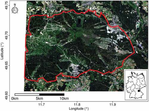
The Grafenwoehr military training area (GTA) is located in the south-east of Germany (Figure 2) and lies at about 450 m (sd = 38 m) above sea level in the natural region Upper Palatine-Upper Main Hills. The long-term average temperature and precipitation are 8.3 ± 0.04°C and 701 ± 4 mm, respectively (1981–2010, mean ± SEM of four weather stations of the German Weather Service (DWD, Deutscher Wetterdienst) in the immediate vicinity). The GTA covers 230 km²; about 85% are part of the Natura 2000 network and contain numerous rare, highly protected habitat types and function as a refuge for many endangered species (Riesch, Stroh, Tonn, & Isselstein, 2018; Warren & Büttner, 2008a, 2008b). About 40% of GTA are covered with open habitats, such as grassland or heath, while about 60% are covered with forest. Parts of the grassland areas are mown once a year around the beginning of July. Wildlife grazing, especially by red deer (Cervus elaphus), also plays an important role for vegetation dynamics (Meißner, Reinecke, Herzog, Leinen, & Brinkmann, 2012).

Figure 2. Location of the study site Grafenwoehr military training area outlined in red. The location of the study site in Germany is marked with a black square in the lower right map. The background map is based on the 24 June 2016 RapidEye acquisition (Table 1)

Satellite data and pre-processing

A multi-temporal RapidEye time-series consisting of ten images covering the years between 2014 and 2017 (Table 1) was acquired. The ordered processing level 3A was already radiometrically, geometrically, and sensor corrected, and was delivered covering one 25 by 25 km tile (ID-3,262,023).

Table 1. Multi-annual RapidEye time-series ordered by adjusted Julian day of the year (DOY)

No	Acquisition date	Actual Julian DOY	Adjusted Julian DOY	Sensing time (am)	Sensor view angle (°)	Phenological phase
1	14 March 2016	74	88	10:45	10.4	prespring (PSP)	DOY 71-102
2	27 March 2017	86	95	10:35	3.5
3	2 April 2014	92	114	11:17	13.0	first spring (FIS)	DOY 103-131
4	20 April 2016	111	119	11:07	9.6
5	17 April 2014	107	127	11:14	6.3
–						full spring (FUS)	DOY 132-158
6	11 June 2017	162	169	10:31	6.9	early summer (ESU)	DOY 159-179
7	24 June 2016	176	183	10:49	0.3	midsummer (MSU)	DOY 180-220
8	25 August 2017	237	243	10:27	3.5	late summer (LSU)	DOY 221-244
–						early autumn (EA)	DOY 245-266
–						full autumn (FA)	DOY 267-284
9	12 October 2015	285	287	11:02	6.3	late autumn (LA)	DOY 285- 305
10	16 October 2017	289	290	10:25	6.6

The pre-processing included a correction of the acquisition dates for shifts in the phenology according to the method proposed by Schmidt et al. (2014). In a multi-annual study context this is an important processing step, because two images from different years, acquired for the same day of the year and the same area, can differ in their phenology. The actual Julian day of the year was corrected for each acquisition to an adjusted Julian day of the year (Table 1), as outlined in Raab et al. (2018).

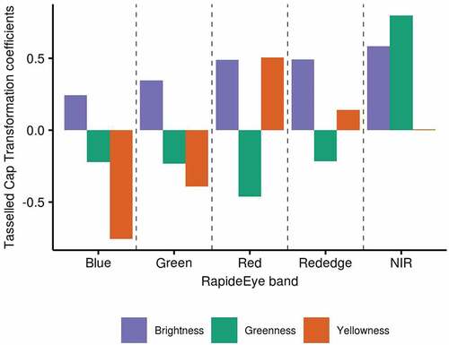
In order to ensure spatial consistency and to reduce potential classification errors all images were co-registered to the image acquired on 2 April 2014 using the function coregisterImages, implemented in the package RStoolbox (Leutner & Horning, 2018) in the R statistical programming environment (R Core Team, 2018). TOA was derived according to the product specification by the data provider (Planet Labs Inc., 2016). The Tasselled-Cap-indices Brightness (TCB), Greenness (TCG), and Yellowness (TCY) were derived from TOA-data using the transformation introduced by Schönert et al. (2014). The band specific weighting factors are illustrated in Figure 3. The SR dataset was derived using the Second Simulation of Satellite Signal in the Solar Spectrum (6S) algorithm (Vermote et al., 1997), implemented in the function i.atcorr within the open source Geographic Resources Analysis Support System (GRASS GIS), version 7.6 (GRASS Development Team, 2019).

Figure 3. Tasselled Cap Transformation coefficients for Brightness, Greenness and Yellowness for each band according to Schönert et al. (2014)

Training and validation data collection

The classification schema was adopted from the Corine Land Cover level 3 classes. The selected classes included water, moors and heathlands, managed grassland, unmanaged grassland, transitional woodland-shrub, broad-leaved forest, coniferous forest and other (Table 2). Because the main focus was on the application of TCT with regard to vegetated land cover the classes artificial surfaces and bare soil were summarised as “other”.

Table 2. Classification schema, respective number of training points and independent validation points

Number	Class name		Number of training points used for cross-validation	Number of independent validation points used for the McNemar test
1	water	WA	120	5
2	moors and heathlands	MH	393	14
3	managed grassland	GM	433	21
4	unmanaged grassland	GU	1059	106
5	broad-leaved forest	BF	561	67
6	coniferous forest	CF	788	156
7	transitional woodland-shrub	TW	316	13
8	other	OS	434	28
	Total		4104	410

An independent validation set of 410 locations was created by a random sampling approach (Table 2). The distinction between different classes was aided by an aerial image (24 June 2016) as well as the habitat map created as part of the Natura 2000 legal obligations in 2006 (Meißner et al., 2012). Similarly, a total of 4104 training locations for cross-validation were distributed over the GTA (Table 2). As recommended by Millard and Richardson (2015), the proportion of training and validation sample locations per class were adjusted to reflect the actual class proportion in the study area, guided by the Natura 2000 habitat map. Plots of TCB, TCG and TCY against adjusted Julian day of the year were used to visualise vegetation phenology for the selected land cover classes using the extracted information at the training set locations (Pasquarella, Holden, Kaufman, & Woodcock, 2016).

Classification and validation

The RF machine learning classifier implemented in the package ranger (Wright & Ziegler, 2015) was used to relate the TCT, TOA and SR predictor variables to the training sample dataset, respectively. The non-parametric method of RF was selected, because it can handle high-dimensional datasets (Belgiu & Drăguţ, 2016) and its robustness for mapping heterogeneous habitats has been demonstrated by several studies (Barrett, Raab, Cawkwell, & Green, 2016; Cutler et al., 2007; Millard & Richardson, 2015; Rodriguez-Galiano, Ghimire, Rogan, Chica-Olmo, & Rigol-Sanchez, 2012). The RF algorithm is an ensemble-based classification tree, from which the predictions are drawn by a majority vote among all trees. The trees are constructed using a subset of training samples drawn through replacement (Belgiu & Drăguţ, 2016). For this, about two thirds of the training samples are used to train the trees (in-bag samples) and the remaining one third is used to estimate the model performance using internal cross-validation (out of bag samples, OOB). As recommended by Belgiu and Drăguţ (2016), the number of trees to be constructed (num.trees) was set to 500. The number of predictor variables randomly sampled as candidates at each split (mtry) was set to the square root of the total number of predictor variables (Gislason, Benediktsson, & Sveinsson, 2006).

In addition to the RF, the C 5.0 algorithm was used in order to compare the performance of RF to a frequently applied tree-based machine learning classification approach (Colditz, 2015; DeFries & Chan, 2000; Shen et al., 2019; Sun, Leinenkugel, Guo, Huang, & Kuenzer, 2017). For this, the package C50 by Kuhn, Weston, Coulter, and Quinlan (2014) was used. The boosting iterations were set to 75 according to initial hyperparameter tuning results using the package mlr. A detailed description of the C5.0 algorithm can be found in Kuhn and Johnson (2013).

To account for the randomness, the classification maps were derived from the most frequently predicted class from 100 spatial predictions per pixel. In addition to the classification map, spatial probability values were derived from, as the mean of 100 predictions.

An important part of land cover classification is the validation, e.g. accuracy assessment by a confusion matrix, of the final map (Foody, 2002). For this, a k-fold cross-validation approach was implemented. The k-fold cross-validation procedure partitions the dataset selected for the model construction randomly into k folds, i.e. k single parts of the dataset. In this approach, k-1 folds are used to train the model and the remaining one fold is used to validate the classification model. This approach has the advantage that, with sufficient repetitions, all the samples can be used to train and validate a model. Hence, a 10-fold cross-validation was used to estimate the models constructed using the training sample set, implemented in the package mlr (Bischl et al., 2016). The validation procedure was repeated 100 times to reduce variance introduced by the cross-validation. Accuracy assessment included overall, user’s and producer’s accuracy, derived from a standard confusion matrix (Congalton, 1991).

The independent validation set of 410 locations (Table 2) was used to compare the statistical significance of the differences between the land cover predictions derived from TCT, TOA and SR data for both algorithms. For this, the non-parametric McNemar test was used (Foody, 2004), which has been commonly applied to evaluate differences between classification results (Barrett et al., 2016; Rodriguez-Galiano et al., 2012). The significance level was set to 5% with a z-critical value of z = 1.96.

Variable importance

Permutation-based variable importance was derived in order to estimate which TCT index, spectral TOA or SR band at which phenological season contributed most to the RF and C 5.0 model performance. By excluding one variable and keeping the rest in the model, the contribution to the performance can be estimated in terms of change in classification error rate (Peña & Brenning, 2015; Ruß & Brenning, 2010). Thus, the increase of classification error as a measure of variable importance was estimated with 100 permutations per variable, using the package mlr.

Results

Tasselled Cap Transformation time-series

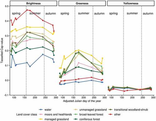
The created training data set was used to extract the TCB, TCG and TCY time-series data and to explore differences in the phenology across the land cover classes. Figure 4 illustrates the seasonal variability with distinct patterns for all eight land cover classes. Values of TCB were generally higher than those of TCG and TCY. The TCY curves showed little variability for all classes with consistently negative values close to zero. The TCG profiles exhibited more pronounced phenological patterns with peaks in the early summer for all classes, except for the non-vegetative ones “other” and “water”. The classes “unmanaged” and “management grassland” were well separated according to the TCB and TCG seasonal profiles. The class “managed grassland” showed consistently higher TCB and TCG values compared to “unmanaged grassland”. Both TCB and TCG curves captured transitions from leaf-on to leaf-off periods for “broad-leaved forest” and “transitional woodland-shrub” with high seasonal amplitude. The highest TCB values were present for the class “other”, which had very low TCG values without a seasonal pattern.

Figure 4. Seasonal Tasselled Cap Brightness, Greenness and Yellowness index plots using the mean value of the extracted training data (Table 2) set per class

Classification and validation

The accuracy assessment results derived from repeated 10-fold cross-validation for the the TCT, TOA and SR datasets are shown in Table 3. The overall accuracy for the RF and all three datasets was about 91.5% (TCT sd = 1.4%, TOA sd = 1.4%, SR sd = 1.3%). Similar performance results were estimated for C 5.0, with overall accuracies ranging from 91.5% for TCT (sd = 1.3%) to 91.8% for TOA and SR (TOA sd = 1.3%, SR sd = 1.3%). The derived Kappa values were very similar in all cases. Class-specific omission and commission error rates are illustrated by producer’s (PA) and user’s accuracy (UA) in Table 3. Lowest PA and UA values were estimated for the classes “transitional woodland-shrub” and “moors and heathlands”. In general, the differences between the three tested datasets and algorithms were small.

Table 3. Classification results for all three datasets. PA = producer’s and UA = user’s accuracy. RF = Random Forests classification, C 5.0 = C 5.0 boosted tree-based classification

	Tasselled Cap Transformation		Top of atmosphere reflectance		Surface reflectance
	RF	C5.0	RF	C5.0	RF	C5.0
Overall Accuracy (%)	91.49	91.44	91.55	91.81	91.49	91.80
Kappa	0.90	0.90	0.90	0.90	0.90	0.90
water
PA	0.97	0.95	0.93	0.94	0.93	0.94
UA	0.97	0.96	0.98	0.99	0.98	0.99
moors and heathlands
PA	0.87	0.89	0.85	0.85	0.85	0.85
UA	0.82	0.85	0.84	0.86	0.84	0.85
managed grassland
PA	0.94	0.94	0.94	0.93	0.94	0.93
UA	0.95	0.96	0.95	0.97	0.95	0.97
unmanaged grassland
PA	0.91	0.90	0.91	0.91	0.91	0.91
UA	0.87	0.87	0.86	0.87	0.86	0.87
broad-leaved forest
PA	0.92	0.90	0.92	0.95	0.92	0.93
UA	0.93	0.92	0.94	0.93	0.94	0.93
coniferous forest
PA	0.96	0.95	0.95	0.95	0.95	0.95
UA	0.94	0.94	0.94	0.94	0.94	0.94
transitional woodland-shrub
PA	0.80	0.83	0.82	0.85	0.81	0.84
UA	0.92	0.90	0.95	0.92	0.95	0.92
other
PA	0.92	0.94	0.95	0.96	0.95	0.96
UA	0.99	0.98	0.98	0.97	0.98	0.97

The results of the McNemar test between the TCT, TOA and SR classification results using the independent validation set (Table 2) for both algorithms are displayed in Table 4. The null hypothesis, i.e. no significant difference between classification results, was confirmed for TOA and SR for the RF. The TCT classification results differed significantly from the TOA and SR results (p < 0.005). For the C 5.0, a similar pattern was observed between TCT and TOA. The overall accuracy estimated by the independent validation set was higher for TCT (RF = 96.34%, C 5.0 = 92.93%) than that of the TOA and SR classification results (RF = 89.8–89.3%, C 5.0 = 89.02–89.51%). A direct comparison between both algorithms showed that only the TCT results differed significantly (p < 0.005).

Table 4. Results of the McNemar test for three different datasets, TCT = Tasselled Cap Transformation, TOA = Top of atmosphere reflectance, SR = surface reflectance, OA = overall accuracy. RF = Random Forests classification, C 5.0 = C 5.0 boosted tree-based classification

Map 1	Map 2	|z|	p value	OA map 1 (%)	OA map 2 (%)	Kappa map 1	Kappa map 2
RF TCT	RF TOA	4.56	< 0.005	96.34	89.76	0.95	0.87
RF TCT	RF SR	4.77	< 0.005	96.34	89.27	0.95	0.86
RF TOA	RF SR	1.41	0.079	89.76	89.27	0.87	0.86
C 5.0 TCT	C 5.0 TOA	2.74	< 0.005	92.93	89.02	0.91	0.86
C 5.0 TCT	C 5.0 SR	2.47	0.007	92.93	89.51	0.91	0.86
C 5.0 TOA	C 5.0 SR	0.71	0.760	89.02	89.51	0.86	0.86
RF TCT	C 5.0 TCT	2.86	< 0.005	96.34	92.93	0.95	0.91
RF TOA	C 5.0 TOA	0.77	0.219	89.76	89.02	0.87	89.51
RF SR	C 5.0 SR	0.23	0.591	89.27	89.51	0.86	0.86

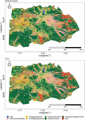
The predicted maps derived from the TCT RF and C 5.0 model are shown in Figure 5. The accompanying predicted probability maps for each class are displayed in the supplemental material Figures S1 and S2. The percentages of all land cover classes are shown in Table 5. The differences between TCT, TOA and SR predicted proportion of the land cover were small, similar to the differences between RF and C 5.0. The dominant vegetation cover classes in all three versions were “coniferous forest” and “broad-leaved forest”, making up about 54% of the total area. Most of the “transitional woodland-shrub” cover was in the western part of the study site, predominantly associated with a more fragmented landscape. Larger complexes of “managed grassland” were embedded in this fragmented mixture of open landscape and “transitional woodland-shrub” and forest. The class “unmanaged grassland” can be found relatively ubiquitously, but with larger complexes in the centre as well as in the western part of the study site. The class “other” covers a larger area in the centre of the study site, which reflects soil scarification due to exploded ordnance. In the eastern part of the study site the class “moors and heathlands” occurred more frequently, compared to the remaining area. This can be related to dryer and less fertile soil conditions for heathlands in the northern and north-eastern part of the study site (Riesch et al., 2018).

Table 5. Share of land cover classes for the Tasselled Cap Transformation (TCT), Top of atmosphere (TOA) and surface reflectance (SR) predicted maps. RF = Random Forests classification, C 5.0 = C 5.0 boosted tree-based classification

Number	Class name	RF			C 5.0
		TCT	TOA	SR	TCT	TOA	SR
		Share of class (%)
1	water	1.26	1.20	1.20	1.25	1.26	1.27
2	moors and heathlands	3.66	3.57	3.59	3.48	3.48	3.45
3	managed grassland	3.69	3.64	3.65	3.79	3.70	3.73
4	unmanaged grassland	26.31	25.42	25.41	25.16	25.15	25.17
5	broad-leaved forest	15.53	16.18	16.16	16.45	16.32	16.15
6	coniferous forest	38.36	38.09	38.12	37.49	37.76	38.00
7	transitional woodland-shrub	2.75	2.61	2.59	3.25	3.13	3.10
8	other	8.44	9.29	9.28	9.13	9.19	9.15
	Total	100

Figure 5. Classification map for the GTA derived from the multi-temporal Tasselled Cap RapidEye times-series, using the Random Forest and C 5.0 classification algorithm, respectively. To improve the homogeneity of the classification a 3 × 3 majority filter was applied to the presented map

Variable importance

The permutation-based variable importance estimated as the mean increase in error rate is shown in Figure 6. For the TOA and SR classification, the most important variable for the RF model was the near-infrared band. This was particularly the case for the phenological seasons early summer and late autumn, which were generally the most important time frames. For the TCT dataset, TCG contributed most to the classification model. The sum of its mean increase in error rate across all considered phenological seasons was about 6.38%. For TCB and TCY, sums of 1.35% and 0.01% were estimated, respectively. The most important phenological season for the TCT model was late autumn. In general, the maximum mean increase in error rate values were higher for the models based on TCT data compared to TOA and SR.

Figure 6. Permutation-based variable importance derived as mean increase in error rate for the top of atmosphere (TOA), surface reflectance (SR) and Tasselled Cap Transformation (TCT) dataset. TCB = Brightness, TCG = Greenness, TCY = Yellowness, PSP = prespring, FIS = first spring, FUS = full spring, ESU = early summer, MSU = midsummer, LSU = late summer, EA =early autumn, FA = full autumn, LA = late autumn

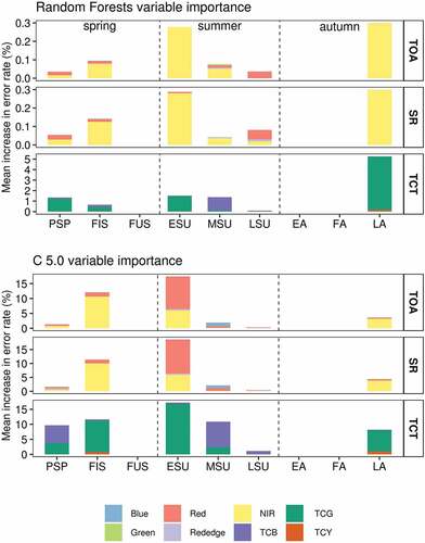
The importance of phenological seasons were similar for the C 5.0 algorithm, except for a lower importance of the late autumn season. For the TOA and SR classification, the most important variable for the C 5.0 model were the near-infrared and rededge bands. In case of the TCT dataset, TCG was the most important variable, followed by TCB and TCY. Across all considered phenological seasons the sum of mean increase in error rate was about 40.28% for TCG, 16.76% for TCB and 1.81% for TCY. In contrast to the RF model, the most important phenological season for the C 5.0 TCT model was the early summer. The magnitude of the variable importance values estimated for the C 5.0 models was higher compared to the models based on the RF algorithm.

Discussion

Tasselled Cap Transformation time-series

Similar to the study by Pasquarella et al. (2016), who evaluated Landsat Tasselled Cap time-series to characterise different habitats, distinct phenological profiles of different land cover classes were provided by the RapidEye TCT time-series (Figure 4). As TCG has a high positive weighting factor for the near-infrared band (Figure 3), it covers the spectral variation of live vegetation well. Thus, all TCG-profiles of vegetated surfaces followed a typical green-up curve, similar to the commonly used normalised difference vegetation index (Pettorelli et al., 2005). Most studied land cover classes showed a peak in TCB at the beginning of summer, especially for the class “other”. As the TCB captures overall brightness and variance in soil brightness (Schönert et al., 2015), this might be attributed to changes in soil conditions, such as moisture.

The Tasselled-Cap-transformed Landsat archive data has been recently recognised as a valuable tool to asses abrupt as well as gradual changes in land cover (Kennedy et al., 2015; Kennedy, Yang, & Cohen, 2010; Pasquarella et al., 2016). The available RapidEye archive data should be considered by future studies to evaluate the potential of the high spatial resolution Tasselled-Cap-transformed RapidEye data for change analysis.

Classification and validation

Only marginal differences in cross-validated classification accuracy between the datasets (TCT, TOA, SR) and algorithms were present (Table 3).

The McNemar test showed no significant difference between the TOA and SR dataset (Table 4) for both algorithms. This was similar to the results provided by Raab, Barrett, Cawkwell, and Green (2015), who reported only marginal classification accuracy differences among different atmospheric correction approaches and uncorrected multi-temporal Landsat data. Even though the study area has only small topographic variability, an additional topographic correction could have increased the predictive power of the classification model (Vanonckelen, Lhermitte, & Van Rompaey, 2013). However, classification results based on TCT differed significantly from both classifications based on untransformed values (excluding the C 5.0 SR dataset), and had a higher overall accuracy than those (Table 4). This might be related to a lower model complexity as a smaller number of predictor variables were included, and to a reduced correlation among the predictor variables in the TCT dataset (Millard & Richardson, 2015). However, as the amount of samples of the independent validation set was limited for some classes (Table 2), the accuracy assessment accompanying the McNemar test should be considered with caution. Nevertheless, the TCT can be considered as an effective data compression approach, which can provide similarly high classification accuracies as TOA and SR data.

Both algorithms showed very high classification accuracies with marginal differences. A similar pattern was observed in a comparison between RF and boosted Decision Trees among others machine learning algorithms (Maxwell, Warner, & Fang, 2018). A variety of alternative land cover classification concepts have been presented using RapidEye data in comparison to the presented pixel-based approach. For land cover mapping with single temporal RapidEye data and machine learning techniques, such as Support Vector Machines, Schuster et al. (2012) and Ustuner, Sanli, and Dixon (2015) reported OA values ranging from 78.1 to 85.6%. More accurate classification results were reported for multi-temporal data (Schuster et al., 2015; Zillmann & Weichelt, 2013), similar to the results presented in this study. However, the application of Support Vector Machines is computational intensive, since it requires parameter tuning. In a direct comparison of Support Vector Machines and RF for land cover classification in a heterogeneous coastal landscape, Adam, Mutanga, Odindi, and Abdel-Rahman (2014) found no significant difference between the performance of both algorithms. The overall accuracy estimated for the RF classification was slightly higher compared to the result using Support Vector Machines. The opposite observation was made by Maxwell, Strager, Warner, Zegre, and Yuill (2014), where SVM outperformed RF for mapping of mining and mine reclamation using RapidEye data. Given these contrary results in the literature the selection of a machine learning algorithm can be seen as a challenging task (Maxwell et al., 2018) and should be considered as dataset dependent (Lawrence & Moran, 2015). However, the systematic comparison among common machine learning algorithms of Lawrence and Moran (2015) showed that the RF was the most accurate algorithm in 18 and the C 5.0 in 11 out of 30 cases.

Variable importance

As most of the surface in the study site was covered with vegetation (Table 5), the high importance of the Greenness TCT-index and the near-infrared and rededge band of the TOA and SR dataset for both algorithms was not surprising. The small contribution of the TCY data can be explained by the small variability of this transformation component (Schönert et al., 2014). However, all components of the respective datasets should be considered for mapping land cover, because a potential interdependence between the predictor variables would otherwise be disregarded. The differences between the TOA and SR variable importances were small. For both datasets, the rededge band contributed to the model accuracy, albeit only slightly. Similar results were reported by Schuster et al. (2012).

The phenological correction of acquisition dates allowed to compare how different phenological phases from different years contributed to the classification model. The phenological seasons early summer and late autumn contributed most to the RF and C 5.0 classification models in all three cases (Figure 6). Therefore, the early summer and late autumn season must be seen as a critical data acquisition window for mapping land cover by the means of satellite remote sensing in this study. This is supported by Förster, Frick, Schuster, and Kleinschmit (2010), who recommended using image acquisitions originating from the onset of vegetation and the senescence phase to map Natura 2000 habitats. As the remote sensing data available in this study did not cover all phenological seasons (Table 1), a broad generalisation concerning the importance of all phenological phases was not possible.

Conclusion

The classification of a heterogeneous landscape using Tasselled-Cap-transformed RapidEye data achieved similar high overall accuracies compared to top of atmosphere and surface reflectance data. Thus, the RapidEye Tasselled Cap Transformation can be seen as an effective data compression measure, valuable for the application of multi-temporal land cover mapping. This can reduce the pre-processing effort in a multi-temporal data context, as the results of Tasselled-Cap-transformed data achieved similar overall accuracies compared to surface reflectance data. Satellite images acquired at the same Julian day of the year from consecutive years can represent different vegetative seasons, caused by climate variabilities. Hence, a phenological correction of image acquisition dates must be seen as a pivotal pre-processing step for the analysis of satellite remote sensing data originating from different years. If not considered, variable importance measures about influential image acquisition timings might be misleading. In this study the Tasselled Cap Transformation captured phenological patterns of vegetated surfaces and the early summer and late autumn were identified as the most influential image acquisition windows. As the results of the Random Forest and C 5.0 approach were very similar, the choice of classification algorithm must be considered as less important for this study case.

Future research should evaluate the potentials of the Tasselled-cap-transformed RapidEye data to study environmental changes at very high resolutions. In this study only clear sky observations were included. Therefore, the influence of e.g. cirrus clouds on the Tasselled Cap Transformation and derived classification results in comparison to different atmospheric correction strategies needs to be addressed in the future.

Acknowledgments

We thank Friederike Riesch and Laura Richter for comments on earlier versions of this manuscript. The project was supported by funds of German government’s Special Purpose Fund held at Landwirtschaftliche Rentenbank (28 RZ 7007). We thank the Federal Forests Division (Bundesforst) of the German Institute for Federal Real Estate (Bundesanstalt für Immobilienaufgaben) and the Institut für Wildbiologie Göttingen und Dresden e.V. for close cooperation and support. We acknowledge the DLR for the delivery of RapidEye images as part of the RapidEye Science Archive (RESA) – proposal 00226.

Disclosure statement

No potential conflict of interest was reported by the authors.

Supplementary material

The supplemental data for this article can be accessed here.

Additional information

Funding

This work was supported by the German government’s Special Purpose Fund held at Landwirtschaftliche Rentenbank [28 RZ 7007].

References

- Adam, E., Mutanga, O., Odindi, J., & Abdel-Rahman, E.M. (2014). Land-use/cover classification in a heterogeneous coastal landscape using RapidEye imagery: Evaluating the performance of random forest and support vector machines classifiers. International Journal of Remote Sensing, 35(10), 3440–3458. doi:10.1080/01431161.2014.903435
- Baig, M.H.A., Zhang, L., Shuai, T., & Tong, Q. (2014). Derivation of a tasselled cap transformation based on Landsat 8 at-satellite reflectance. Remote Sensing Letters, 5(5), 423–431. doi:10.1080/2150704X.2014.915434
- Barrett, B., Raab, C., Cawkwell, F., & Green, S. (2016). Upland vegetation mapping using Random Forests with optical and radar satellite data. Remote Sensing in Ecology and Conservation, 2(4), 212–231. doi:10.1002/rse2.32
- Belgiu, M., & Drăguţ, L. (2016). Random forest in remote sensing: A review of applications and future directions. ISPRS Journal of Photogrammetry and Remote Sensing, 114, 24–31. doi:10.1016/j.isprsjprs.2016.01.011
- Bischl, B., Lang, M., Kotthoff, L., Schiffner, J., Richter, J., Studerus, E., … Jones, Z.M. (2016). mlr: Machine learning in R. Journal of Machine Learning Research, 17(170), 1–5.
- Breiman, L. (2001). Random forests. Machine Learning, 45(1), 5–32. doi:10.1023/A:1010933404324
- Colditz, R.R. (2015). An evaluation of different training sample allocation schemes for discrete and continuous land cover classification using decision tree-based algorithms. Remote Sensing, 7(8), 9655–9681. doi:10.3390/rs70809655
- Congalton, R.G. (1991). A review of assessing the accuracy of classifications of remotely sensed data. Remote Sensing of Environment, 37(1), 35–46. doi:10.1016/0034-4257(91)90048-B
- Cortes, C., & Vapnik, V. (1995). Support-vector networks. Machine Learning, 20(3), 273–297. doi:10.1007/BF00994018
- Crist, E.P., & Cicone, R.C. (1984). Application of the tasseled cap concept to simulated thematic mapper data. Ann Arbor, 1001, 48107.
- Cutler, D.R., Edwards, T.C., Beard, K.H., Cutler, A., Hess, K.T., Gibson, J., & Lawler, J.J. (2007). Random forests for classification in ecology. Ecology, 88(11), 2783–2792. doi:10.1890/07-0539.1
- Dahms, T., Seissiger, S., Borg, E., Vajen, H., Fichtelmann, B., & Conrad, C. (2016). Important variables of a RapidEye time series for modelling biophysical parameters of winter wheat. Photogrammetrie-Fernerkundung-Geoinformation, 2016(5–6), 285–299. doi:10.1127/pfg/2016/0303
- DeFries, R.S., & Chan, J.C.-W. (2000). Multiple criteria for evaluating machine learning algorithms for land cover classification from satellite data. Remote Sensing of Environment, 74(3), 503–515. doi:10.1016/S0034-4257(00)00142-5
- Einzmann, K., Immitzer, M., Böck, S., Bauer, O., Schmitt, A., & Atzberger, C. (2017). Windthrow detection in European forests with very high-resolution optical data. Forests, 8(1), 21. doi:10.3390/f8010021
- Foody, G.M. (2002). Status of land cover classification accuracy assessment. Remote Sensing of Environment, 80(1), 185–201. doi:10.1016/S0034-4257(01)00295-4
- Foody, G.M. (2004). Thematic map comparison. Photogrammetric Engineering & Remote Sensing, 70(5), 627–633. doi:10.14358/PERS.70.5.627
- Förster, M., Frick, A., Schuster, C., & Kleinschmit, B. (2010). Object-based change detection analysis for the monitoring of habitats in the framework of the NATURA 2000 directive with multi-temporal satellite data. The International Archives of the Photogrammetry, Remote Sensing and Spatial Information Sciences, 38, 4.
- Gislason, P.O., Benediktsson, J.A., & Sveinsson, J.R. (2006). Random forests for land cover classification. Pattern Recognition Letters, 27(4), 294–300. doi:10.1016/j.patrec.2005.08.011
- Gómez, C., White, J.C., & Wulder, M.A. (2016). Optical remotely sensed time series data for land cover classification: A review. ISPRS Journal of Photogrammetry and Remote Sensing, 116, 55–72. doi:10.1016/j.isprsjprs.2016.03.008
- GRASS Development Team. (2019). Geographic resources analysis support system (GRASS GIS) software, version 7.6. Retrieved from http://grass.osgeo.org
- Houghton, R.A., House, J.I., Pongratz, J., Van Der Werf, G.R., DeFries, R.S., Hansen, M.C., … Ramankutty, N. (2012). Carbon emissions from land use and land-cover change. Biogeosciences, 9(12), 5125–5142. doi:10.5194/bg-9-5125-2012
- Huang, C., Wylie, B., Yang, L., Homer, C., & Zylstra, G. (2002). Derivation of a tasselled cap transformation based on Landsat 7 at-satellite reflectance. International Journal of Remote Sensing, 23(8), 1741–1748. doi:10.1080/01431160110106113
- Kauth, R.J., & Thomas, G.S. (1976). The tasselled cap–A graphic description of the spectral-temporal development of agricultural crops as seen by Landsat. In LARS Symposia, p. 159.
- Kennedy, R.E., Yang, Z., Braaten, J., Copass, C., Antonova, N., Jordan, C., & Nelson, P. (2015). Attribution of disturbance change agent from Landsat time-series in support of habitat monitoring in the Puget Sound region, USA. Remote Sensing of Environment, 166, 271–285. doi:10.1016/j.rse.2015.05.005
- Kennedy, R.E., Yang, Z., & Cohen, W.B. (2010). Detecting trends in forest disturbance and recovery using yearly Landsat time series: 1. LandTrendr—Temporal segmentation algorithms. Remote Sensing of Environment, 114(12), 2897–2910. doi:10.1016/j.rse.2010.07.008
- Kuhn, M., & Johnson, K. (2013). Applied predictive modeling (Vol. 26). New York, NY: Springer.
- Kuhn, M., Weston, S., Coulter, N., & Quinlan, R. (2014). C50: C5. 0 decision trees and rule-based models. R Package Version 0.1. 0-21. Retrieved from http://CRAN. R-Project. Org/Package C, 50
- Lawrence, R.L., & Moran, C.J. (2015). The AmericaView classification methods accuracy comparison project: A rigorous approach for model selection. Remote Sensing of Environment, 170, 115–120. doi:10.1016/j.rse.2015.09.008
- Leutner, B., & Horning, N. (2018). RStoolbox: Tools for remote sensing data analysis. R Package Version 0.2.4.
- Lobser, S.E., & Cohen, W.B. (2007). MODIS tasselled cap: Land cover characteristics expressed through transformed MODIS data. International Journal of Remote Sensing, 28(22), 5079–5101. doi:10.1080/01431160701253303
- Löw, F., Fliemann, E., Abdullaev, I., Conrad, C., & Lamers, J.P. (2015). Mapping abandoned agricultural land in Kyzyl-Orda, Kazakhstan using satellite remote sensing. Applied Geography, 62, 377–390. doi:10.1016/j.apgeog.2015.05.009
- Maxwell, A. E., Strager, M. P., Warner, T. A., Zégre, N. P., & Yuill, C. B. (2014). Comparison of naip orthophotography and rapideye satellite imagery for mapping of mining and mine reclamation. Giscience & Remote Sensing, 51(3), 301-320.
- Maxwell, A.E., Warner, T.A., & Fang, F. (2018). Implementation of machine-learning classification in remote sensing: An applied review. International Journal of Remote Sensing, 39(9), 2784–2817. doi:10.1080/01431161.2018.1433343
- Meißner, M., Reinecke, H., Herzog, S., Leinen, L., & Brinkmann, G. (2012). Vom Wald ins Offenland: Der Rothirsch auf dem Truppenübungsplatz Grafenwöhr. Raum-Zeit-Verhalten, Lebensraumnutzung, Management (1. Aufl). Ahnatal: Frank Fornacon.
- Millard, K., & Richardson, M. (2015). On the importance of training data sample selection in Random Forest image classification: A case study in peatland ecosystem mapping. Remote Sensing, 7(7), 8489–8515. doi:10.3390/rs70708489
- Nitze, I., Barrett, B., & Cawkwell, F. (2015). Temporal optimisation of image acquisition for land cover classification with Random Forest and MODIS time-series. International Journal of Applied Earth Observation and Geoinformation, 34, 136–146. doi:10.1016/j.jag.2014.08.001
- Pasquarella, V.J., Holden, C.E., Kaufman, L., & Woodcock, C.E. (2016). From imagery to ecology: Leveraging time series of all available Landsat observations to map and monitor ecosystem state and dynamics. Remote Sensing in Ecology and Conservation, 2(3), 152–170. doi:10.1002/rse2.24
- Peña, M.A., & Brenning, A. (2015). Assessing fruit-tree crop classification from Landsat-8 time series for the Maipo Valley, Chile. Remote Sensing of Environment, 171, 234–244. doi:10.1016/j.rse.2015.10.029
- Pettorelli, N., Vik, J.O., Mysterud, A., Gaillard, J.-M., Tucker, C.J., & Stenseth, N.C. (2005). Using the satellite-derived NDVI to assess ecological responses to environmental change. Trends in Ecology & Evolution, 20(9), 503–510. doi:10.1016/j.tree.2005.05.011
- Planet Labs Inc. (2016). Satellite imagery product specifications. Satellite Imagery Product Specifications: Version 6.1.
- R Core Team. (2018). R: A Language and Environment for Statistical Computing. Retrieved from https://www.R-project.org/
- Raab, C., Barrett, B., Cawkwell, F., & Green, S. (2015). Evaluation of multi-temporal and multi-sensor atmospheric correction strategies for land-cover accounting and monitoring in Ireland. Remote Sensing Letters, 6(10), 784–793. doi:10.1080/2150704X.2015.1076950
- Raab, C., Stroh, H.G., Tonn, B., Meißner, M., Rohwer, N., Balkenhol, N., & Isselstein, J. (2018). Mapping semi-natural grassland communities using multi-temporal RapidEye remote sensing data. International Journal of Remote Sensing, 39(17), 5638–5659. doi:10.1080/01431161.2018.1504344
- Riesch, F., Stroh, H.G., Tonn, B., & Isselstein, J. (2018). Soil pH and phosphorus drive species composition and richness in semi-natural heathlands and grasslands unaffected by twentieth-century agricultural intensification. Plant Ecology & Diversity, 11(2), 239–253. doi:10.1080/17550874.2018.1471627
- Rodriguez-Galiano, V.F., Ghimire, B., Rogan, J., Chica-Olmo, M., & Rigol-Sanchez, J.P. (2012). An assessment of the effectiveness of a random forest classifier for land-cover classification. ISPRS Journal of Photogrammetry and Remote Sensing, 67, 93–104. doi:10.1016/j.isprsjprs.2011.11.002
- Ruß, G., & Brenning, A. (2010). Spatial variable importance assessment for yield prediction in precision agriculture. In Advances in intelligent data analysis IX (pp. 184–195).
- Schmidt, T., Schuster, C., Kleinschmit, B., & Förster, M. (2014). Evaluating an intra-annual time series for grassland classification—How many acquisitions and what seasonal origin are optimal? IEEE Journal of Selected Topics in Applied Earth Observations and Remote Sensing, 7(8), 3428–3439. doi:10.1109/JSTARS.2014.2347203
- Schönert, M., Weichelt, H., Zillmann, E., & Jürgens, C. (2014). Derivation of tasseled cap coefficients for RapidEye data. SPIE Remote Sensing (pp. 92450Q–92450Q). International Society for Optics and Photonics. Event: SPIE Remote Sensing, 2014, Amsterdam, Netherlands.
- Schönert, M., Zillmann, E., Weichelt, H., Eitel, J.U.H., Magney, T.S., Lilienthal, H., … Jarmer, T. (2015). The tasseled cap transformation for RapidEye data and the estimation of vital and senescent crop parameters. The International Archives of Photogrammetry, Remote Sensing and Spatial Information Sciences, 40(7), 101. doi:10.5194/isprsarchives-XL-7-W3-101-2015
- Schuster, C., Förster, M., & Kleinschmit, B. (2012). Testing the red edge channel for improving land-use classifications based on high-resolution multi-spectral satellite data. International Journal of Remote Sensing, 33(17), 5583–5599. doi:10.1080/01431161.2012.666812
- Schuster, C., Schmidt, T., Conrad, C., Kleinschmit, B., & Förster, M. (2015). Grassland habitat mapping by intra-annual time series analysis–Comparison of RapidEye and TerraSAR-X satellite data. International Journal of Applied Earth Observation and Geoinformation, 34, 25–34. doi:10.1016/j.jag.2014.06.004
- Shen, W., Li, M., Huang, C., Tao, X., Li, S., & Wei, A. (2019). Mapping annual forest change due to afforestation in Guangdong Province of China using active and passive remote sensing data. Remote Sensing, 11(5), 490. doi:10.3390/rs11050490
- Song, C., Woodcock, C.E., Seto, K.C., Lenney, M.P., & Macomber, S.A. (2001). Classification and change detection using Landsat TM data: When and how to correct atmospheric effects? Remote Sensing of Environment, 75(2), 230–244. doi:10.1016/S0034-4257(00)00169-3
- Sun, Z., Leinenkugel, P., Guo, H., Huang, C., & Kuenzer, C. (2017). Extracting distribution and expansion of rubber plantations from Landsat imagery using the C5. 0 decision tree method. Journal of Applied Remote Sensing, 11(2), 026011. doi:10.1117/1.JRS.11.026011
- Tyc, G., Tulip, J., Schulten, D., Krischke, M., & Oxfort, M. (2005). The RapidEye mission design. Acta Astronautica, 56(1), 213–219. doi:10.1016/j.actaastro.2004.09.029
- Ustuner, M., Sanli, F.B., & Dixon, B. (2015). Application of support vector machines for landuse classification using high-resolution RapidEye images: A sensitivity analysis. European Journal of Remote Sensing, 48(1), 403–422. doi:10.5721/EuJRS20154823
- Vanonckelen, S., Lhermitte, S., & Van Rompaey, A. (2013). The effect of atmospheric and topographic correction methods on land cover classification accuracy. International Journal of Applied Earth Observation and Geoinformation, 24, 9–21. doi:10.1016/j.jag.2013.02.003
- Vermote, E.F., Tanré, D., Deuze, J.L., Herman, M., & Morcette, -J.-J. (1997). Second simulation of the satellite signal in the solar spectrum, 6S: An overview. IEEE Transactions on Geoscience and Remote Sensing, 35(3), 675–686. doi:10.1109/36.581987
- Warren, S.D., & Büttner, R. (2008a). Active military training areas as refugia for disturbance-dependent endangered insects. Journal of Insect Conservation, 12(6), 671–676. doi:10.1007/s10841-007-9109-2
- Warren, S.D., & Büttner, R. (2008b). Relationship of endangered amphibians to landscape disturbance. Journal of Wildlife Management, 72(3), 738–744. doi:10.2193/2007-160
- Wilson, R.T., Milton, E.J., & Nield, J.M. (2014). Spatial variability of the atmosphere over southern England, and its effect on scene-based atmospheric corrections. International Journal of Remote Sensing, 35(13), 5198–5218. doi:10.1080/01431161.2014.939781
- Wright, M.N., & Ziegler, A. (2015). ranger: A fast implementation of random forests for high dimensional data in C++ and R. In: J. Stat. Soft. 77 (1). doi:10.18637/jss.v077.i01.
- Zillmann, E., & Weichelt, H. (2013). Grassland identification using multi-temporal RapidEye image series. Analysis of Multi-Temporal Remote Sensing Images, MultiTemp 2013: 7th International Workshop on The (pp. 1–4), Banff, AB, Canada. Retrieved from http://ieeexplore.ieee.org/abstract/document/6866011/