A rule-based model for Seoul Bike sharing demand prediction using weather data

1

ABSTRACT

This research paper presents a rule-based regression predictive model for bike sharing demand prediction. In recent days, Pubic rental bike sharing is becoming popular because of is increased comfortableness and environmental sustainability. Data used include Seoul Bike and Capital Bikeshare program data. Both data have weather data associated with it for each hour. For both the dataset, five statistical models were trained with optimized hyperparameters using a repeated cross validation approach and testing set is used for evaluation: (a) CUBIST (b) Regularized Random Forest (c) Classification and Regression Trees (d) K Nearest Neighbour (e) Conditional Inference Tree. Multiple evaluation indices such as R², Root Mean Squared Error, Mean Absolute Error and Coefficient of Variation were used to measure the prediction performance of the regression models. The results show that the rule-based model CUBIST was able to explain about 95 and 89% of the Variance (R²) in the testing set of Seoul Bike data and Capital Bikeshare program data respectively. An analysis with variable importance was carried to analyse the most significant variables for all the models developed with the two datasets considered. The variable importance results have shown that Temperature and Hour of the day are the most influential variables in the hourly rental bike demand prediction.

KEYWORDS:

• Data Mining
• GIS
• predive analytics
• intelligent transport system

Introduction

In a span of few decade, the sharing of bicycle system has seen enamours growth (Fishman, 2016). This system is a recently developed transportation system which provides people with bicycle for common use. Bicycle system provides user to rent a bike from one docking station, where user can ride and then return in another docking station. Amsterdam in Netherlands was the one where initial bicycle sharing system has started in 1965 (Shaheen, Guzman, & Zhang, 2010). Main motive of the system was to focus on environmental and social welfare. With enormous advancement of Intelligent Transportation System and information technology after 2000s, this bicycle system employed globally. Situation over decade has changed in sharing bicycle. Today it is much easier for the public to rent bicycles. Global Positioning System enabled mobile application allows people to know the nearby bicycle station for renting the bicycle.

Till today there are more than 50 countries having 712 which implemented bicycle sharing method (Shaheen, Martin, Cohen, Chan, & Pogodzinski, 2014). They have now found to be important face of transportation system in major cities due to several factors such as health problems, heavy traffic and environmental conditions. Bike sharing Systems namely OFO and Mo-bike in places like Beijing has enabled people to find position of unused bicycle and use them. Once the bicycle is used, it can be locked at any docking station across the city. For expanding availability of bicycle for public use, the operators running this service allocate a truck that collects bicycles parked in various station and relocate them to the original station gradually (Schuijbroek, Hampshire, & Van Hoeve, 2017). There are number of policy issues involved in the management of intelligent bicycle sharing system (Gast, Massonnet, Reijsbergen, & Tribastone, 2015).

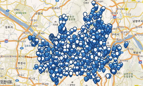
Many countries have bike sharing system, such as Ddareungi is a bike sharing system in South Korea, which started in the year 2015, known as Seoul bike in English. It was started to overcome issues like greater oil prices, congestion in traffic and pollution in the environment and to develop a healthy environment for citizen of Seoul to live. Han River is the initial place where Ddareungi was first started on October 2015 in Seoul, few months later, total number of bike sharing station touched 150 with as much as 1500 were there. In order to cover the entire people in Seoul, in 2016 there is a gradual incline in number of docking station. As large as 20,000 bikes were made available which was confirmed by Seoul Mayor Park won-soon. With the help of growing technologies, Seoul city is now equipped with 1500 bike renting station which are operational round the clock. With the help of internet-enabled device or mobile phone, people can know the number of bikes available for the people to rent. Bike are locked which can be unlocked with the help of password which people accessing to it will receive the password through mail. Users are allowed and can rent and leave the bike in any station. Seoul Rental Bikes are built to be utilized by all kinds of people including women, elderly persons and infirm. Seoul Bikes are manufactured using durable and light-weight materials. This giving user more stability in driving and convenience. These public bikes are made available to the persons who are 15 and older. Seoul bike docking stations are equipped in excessive traffic areas including subway entrances/exits, bus stops, residential complexes, public offices, schools, and banks. Docking stations are computerized stands for the purpose of pickup and dropoff of the rental bikes. Users of Seoul public bikes can rent and return rental bikes at any docking station. Users can verify their trip details (distance, duration) and measure of bodily activities (burnt calories) at My Page > Usage Details. With this kind of smart technology and convenience, the use of Rental bike is increasing every day. So, there is a need to manage the bike rental demand and manage the continuous and convenient service for the users. This study proposes a data mining-based approach including weather data to predict whole city public bike demand. A rule-based model is used to predict the number of rental bikes needed at each hour. Figure 1 presents the picture of rental bike stations in Seoul.

Figure 1. Docking stations in Seoul.

The sections in the paper is structured as follows. Section 2 presents the reviews of previous studies related to public bike-sharing systems and prediction algorithms and methods. Section 3 provides detailed information about the algorithms used in this paper. Section 4 provides evaluation indices used for evaluating the algorithms. Section 5 details the data preparation process. Section 6 describes the model development process. Section 7 deals with discussion of results and Finally the paper is concluded in Section 8.

Review of literature works

Nowadays, bike sharing system is an interesting study topic. Number of studies are carried out to know the features and interesting information about it. For instance, Studies are done to enhance the background information about the bike sharing systems, explaining from the starting era of bike sharing to the latest generation approaches (DeMaio, 2009). Fishman mentioned the research carried out on the categories of bicycle sharing system, consisting of the history of the documentation process, usage analysis, user relevance, mentioning the fact that some researchers used automated computerised devices for gathering data related to bicycle sharing system (Fishman, 2016). With enormous incline in the bicycle sharing systems, large number of researches developed approaches for managing their rebalancing procedures. Researches also proposed an active public bike sharing issue based on daily methods consisting of systems, whereas an innovative strategy for managing rental bicycle stations and number of models to solve the problem is also developed (Raviv & Kolka, 2013). To deal with the rebalancing issue, researches have done in the case of predicting the rental bike demand, which could bring better rebalancing procedures. A rebalancing algorithm is developed for the shared bike system efficiently, which focuses on reaching the destination inventory for total of bicycles in individual station (Erdoğan, Battarra, & Calvo, 2015). These examinations have exhibited ways to deal with enhancing the bike station areas, and strategies for stock rebalancing and directing the trucks to redistribute bikes considering spatial and temporal variations. Information recorded by bike sharing frameworks to predict the medium-term request, expecting to help and enhance key and operational planning by means data mining. (Vogel & Mattfeld, 2011). A Geographic Information System (GIS)-based technique for predicting the potential demand as an initial move towards enhancing the station areas for Madrid’s bike sharing system, utilizing population and employment information to compute the spatial demand dissemination (García-Palomares, Gutiérrez, & Latorre, 2012). The Objective of bike sharing frameworks must be to fulfil client request while lessening operational costs, underscoring the significance of anticipating future client request and bike accessibility dependent on information investigation and measurements (Kadri, Kacem, & Labadi, 2016). Consolidated two parts of the issue that had recently been taken care of independently: deciding each station administration level necessities and planning ideal vehicle courses to bike stock rebalancing (Schuijbroek et al., 2017).

Foreseeing the rental bike demand is a significant piece of any rebalancing system, such many researches have concentrated on this problem. Predictive models for evaluating the probable range of complete bike request in a given geographic zone dependent on information from drive to-work studies are created (Barnes & Krizek, 2005). A statistical model for predicting the quantity of bikes hired every hour, which included a few factors considering the quantity of subscribers, the time information during the week, the event of strikes or holidays, and the climate (temperature, measure of rain) (Borgnat, Abry, Flandrin, & Rouquier, 2009). Researchers also examined human mobility information dependent on the quantities of bikes accessible in the stations, utilizing this to identify temporal and geographical patterns of mobility inside the city and predict the quantity of bikes accessible in any provided station minutes or hours in advance (Kaltenbrunner, Meza, Grivolla, Codina, & Banchs, 2010). A technique for assessing the potential demand to determine the location of stations for getting and dropping off bikes with the help of a GIS (Meng, 2011). The impact of climate and calendar events was also considered for the number of trips for all City Cycle stations in Brisbane utilizing a Poisson model (Corcoran, Li, Rohde, Charles-Edwards, & Mateo-Babiano, 2014). Gast et al. utilized probabilistic predictions acquired from a time-inhomogeneous queuing model to figure future bike accessibility in bike sharing framework stations (Gast et al., 2015).

Recently, it is found that the rental bike sharing infrastructure, (for example, cycle paths and ways) affected the rental demand, additionally uncovering huge connections amongst temperature factor and land use and bike sharing action (El-Assi, Mahmoud, & Habib, 2017). Future accessibility of bikes in the stations was predicted by examining the moment of a continuous time Markov-chain population model with time-dependent rates (Feng, Hillston, & Reijsbergen, 2017). Investigation was carried out to study various climate conditions and temporal qualities, in station-level and framework level examination attributes. In the practical station-level examination, researchers utilized a clustering strategy to distinguish gatherings of stations with identical properties, considering the impact of temperature and humidity by presenting a temperature–humidity index and a heat wave marker variable. They likewise completed a system level examination, indicating that specific variables had critical impacts at various occasions of day. Specifically, temperature variable, rainfall, and whether it was a workday effect affected the rental bike demand at specific occasions (Kim, 2018).

In any case, many factors that contribute to the public rental bike demand cannot be precisely predicted utilizing regression-based algorithms. By utilizing the improvement of Artificial neural systems, numerous analysts have demonstrated that Neural network algorithms can beat conventional prediction techniques (Chen, 2003). With Artificial neural networks, Back Propagation Networks were proposed to broaden the scope of issues that can be handled (Russell & Norvig, 2016) and have since been utilized for forecast in a wide variety of regions. Artificial Intelligence and data mining techniques have likewise been applied to the artificial neural network models to enhance the accuracy (Chen, 2007; Tirkel, 2011). The main drawback of using artificial neural network is its complicated structure and computational cost. Deep learning strategies also employed in bike sharing demand prediction.

Although numerous examinations have researched traffic stream and public rental bike demand prediction, only a few have been focussed about the moment-based demand in public bike sharing systems (Gao & Lee, 2019). Furthermore, the continuous variation in bike sharing framework is exceptionally unpredictable and additionally influenced by numerous external factors. Explaining these connections are so intricate is that these factors are continually changing. We research the issue of predicting and analysing the public rental bike demand in a bike sharing framework utilizing data mining approach considering weather information. Five statistical algorithms: (a) CUBIST (b) Regularized Random Forest (c) Classification and Regression Trees (d) K Nearest Neighbour (e) Conditional Inference Tree are used for comparison. All the models are trained with best hyperparameters selected from repeated cross validation approach. Two bike sharing datasets such as Seoul Bike data set and Capital Bikeshare program data are considered in this study. Finally, a variable analysis was done to analyse the most influential variables in each of the regression algorithms considered.

Methodology

Although the data used must be kept in private, it will be important to compare the results with other conventional machine learning algorithms to signify the importance of positives and negatives of each method considered in this study. This section briefly explains the algorithms used in this study. Also, there is no single machine-learning algorithm, which must be optimally applied for every scenario (Wolpert & Macready, 1997). Therefore, five prediction algorithms were considered in this study to compare their performance with each other.

CUBIST

The Cubist model is introduced on the basis of Quinlan’s M5 model tree (Kuhn & Johnson, 2013; Kuhn, Weston, Keefer, Coulter, & Quinlan, 2014; Quinlan, 1992, 1993; Wang & Witten, 1996). The Cubist method creates a series of “if-after-after” rules. Each rule has an associated linear multivariate model. As long as the set of covariates satisfies the conditions of the rule, the corresponding model shall be used to calculate the predicted value. The main advantage of the Cubist method is the addition of multiple training committees and neighbours to make weights more balanced. By means of this, a series of trees are produced to establish the Cubist model. The number of neighbours is used to modify rule-based forecasts. The Cubist model uses a linear combination of the two models. The general conception about the Cubist regression model is described as follows: during the growth of a tree, many leaves and branches have been grown. The branches can be considered as a series of “if- then” rules, while the terminal leaves can be considered as an associated multivariate linear model. Assuming that a number of covariates comply with the condition of a rule, the associated model will be applied to measure the predictive value. The Cubist model adds boosting with training committees (usually greater than one) that is similar to the method of “boosting” by sequentially developing a number of trees with adjusted weights. The number of neighbours in the Cubist model is used to amend the rule-based prediction. In the Cubist model, the models generated by two linear models are expressed as in the Eq. (1)(1) $\zeta \mathrm{p}\mathrm{a}\mathrm{r}=\left(1-a\right)*\zeta \left(p\right)+\mathrm{a}\ast \zeta \left(c\right)$(1) :

(1) $\zeta \mathrm{p}\mathrm{a}\mathrm{r}=\left(1-a\right)*\zeta \left(p\right)+\mathrm{a}\ast \zeta \left(c\right)$(1)

where ζ(c) is the prediction from the current model and ζ(p) is the prediction from the parent model located above it in the tree.

To make the Cubist model easy to interpret, it can be seen as a model that consisting of number of rules in which the relevant multivariate linear mode is attached to each rule. For the case in that the condition of the rule are matched, the associated model shall be assigned to measure a relevant predicted value. The benefit of the Cubist model is that it is a appropriate tool for fresh learners who only have a basis knowledge of statistical learning or machine learning. The Cubist model has also been shown to be a viable method of regression and can be applied to a variety of issues.

Regularized random forest

The Random Forests (RF) technique was among the best ensemble learning strategies for both classification and regression-based tasks (Breiman, 2001). This methodology clearly addresses the high dimensionality of the input information and the general, characteristic non-linearity of the characterization examined. In any case, RF is a most powerful prediction tool for lessening dimensionality since it perceives the significance of each component for the job needing to be done (Chen & Ishwaran, 2012).

Keeping the data set X as a training data set with n number of model in which every sample has p feature, X may be inferred as a matrix [X,j] i$\in$1 … .n, j$\in$1 … .p associated with the vector brands Y seen as [y_i] i$\in$1 … .n, having the focus on choosing of features below, we represent X as [x₁, … … .x_n], i.e, x_j indicates the vector of feature j.

The importance of feature j in RF is established as in the Eq. (2)(2) $\mathrm{i}\mathrm{m}\mathrm{p}\mathrm{o}\mathrm{r}\mathrm{t}\mathrm{a}\mathrm{n}\mathrm{c}{\mathrm{e}}_j=\frac{1}{\mathrm{\#}trees}{\sum }_{v\in x_j}Gain(x_j,v)$(2) :

(2) $\mathrm{i}\mathrm{m}\mathrm{p}\mathrm{o}\mathrm{r}\mathrm{t}\mathrm{a}\mathrm{n}\mathrm{c}{\mathrm{e}}_j=\frac{1}{\mathrm{\#}trees}{\sum }_{v\in x_j}Gain(x_j,v)$(2)

Here, Gain(x_j, v) was the per-node gain in the Gini index of each feature (x_j) and node (v) combination and #trees is the number of trees in the ensemble. The utilization of RF for feature selection technique incorporates the fixing of K, the number of features or variables to picked or a threshold value of feature importance. These issues are overwhelmed by the utilization of regularization. Regularized Random Forest (RRF) strategy chooses the quantity of highlights utilizing a regularization parameter for each component (Deng & Runger, 2013). This parameter keeps up the increasing (Eq. (3(3) $\mathrm{G}\mathrm{a}\mathrm{i}{\mathrm{n}}_{\mathrm{R}\mathrm{R}\mathrm{F}}\left({\mathrm{x}}_{\mathrm{j},}\mathrm{v}\right)=\left\{\begin{array}{c}Gain\left(x_j,v\right)ifjϵF\\ {\propto }_{j}Gain\left(x_j,v\right)ifjnotϵF\end{array}\right.$(3) )) the highlights chose in past hubs and rebuffs the increase of new highlights.

The importance of the RRF feature is described in the Eq. (3)(3) $\mathrm{G}\mathrm{a}\mathrm{i}{\mathrm{n}}_{\mathrm{R}\mathrm{R}\mathrm{F}}\left({\mathrm{x}}_{\mathrm{j},}\mathrm{v}\right)=\left\{\begin{array}{c}Gain\left(x_j,v\right)ifjϵF\\ {\propto }_{j}Gain\left(x_j,v\right)ifjnotϵF\end{array}\right.$(3) :

(3) $\mathrm{G}\mathrm{a}\mathrm{i}{\mathrm{n}}_{\mathrm{R}\mathrm{R}\mathrm{F}}\left({\mathrm{x}}_{\mathrm{j},}\mathrm{v}\right)=\left\{\begin{array}{c}Gain\left(x_j,v\right)ifjϵF\\ {\propto }_{j}Gain\left(x_j,v\right)ifjnotϵF\end{array}\right.$(3)

Here, F is the set of features used to separate in previous nodes and α_j is the regularization parameter for each feature, determined by the Eq. (4)(4) ${\alpha }_j=\left(1-\gamma \right)+\gamma \frac{importanc{e}_j}{ma{x}_{j=1,\dots ,p}\left(importanc{e}_J\right)}$(4) :

(4) ${\alpha }_j=\left(1-\gamma \right)+\gamma \frac{importanc{e}_j}{ma{x}_{j=1,\dots ,p}\left(importanc{e}_J\right)}$(4)

Where γ ∈ [0, 1] was the weight of the normalized importance and when γ = 0 the RRF diminishes by the RF technique. Taking Eq. (4)(4) ${\alpha }_j=\left(1-\gamma \right)+\gamma \frac{importanc{e}_j}{ma{x}_{j=1,\dots ,p}\left(importanc{e}_J\right)}$(4) into account, RRF chooses the features in a straightforward way: 1) Train the RF to acquire the significance of the feature 2) Calculate the best weight parameter (γ*) and afterward, the regularization parameter (αj) to acquire the minimized list of capabilities by RRF. 3) Train another RF with the features chosen. Since RRF has extra advantage by having regularized function and performance is considerably high compared with usual Random Forest, RRF method is used in this study.

Classification and regression trees

Classification and Regression Trees (CART) is a decision tree strategy for building a regression or classification tree based on its dependent variable structure, which might be categorical/factor or numerical/continuous (Breiman, 2017). In the rule-based CART, information is isolated into two subsets with the end goal that the new subset records have higher homogeneity, i.e. higher pureness, comparative with those in the past subset. The accomplishment of the rule of homogeneity includes a recursive isolating technique. A CART is adequately flexible to think about the costs misclassification and to characterize the earlier conveyance of likelihood in the characterization issue. As far as their rationale rules, choice tree models are particularly better than other demonstrating procedures. Purity is portrayed as the consistency among values and target measures in a CART model and is viewed as flawless when all subset esteems are indistinguishable. Three impurity influence measures can be utilized for target field to find split parts for CART models. Also, the dependent field is symbolized utilizing Gini while the least squared deviation model is utilized to automatically select the target field. The Gini index g(t) at the node t of the CART is characterized by the below conditions (5) and (6):

(5) ${\mathrm{h}\left(\mathrm{t}\right)=\sum }_{a\ne b}x\left(a|t\right)x\left(b|t\right)$(5)

(6) $\mathrm{x}\left(\mathrm{a}|\mathrm{t}\right)=\frac{x(a|t)}{x\left(t\right)};x\left(a,t\right)=\frac{\pi \left(a\right)N_a\left(t\right)}{N_a};andx\left(t\right)=\sum _{a}x\left(a,t\right).$(6)

Where a and b are the target field categories. $\pi \left(a\right)$ is the prior probability value for category a, $N_a\left(t\right)$ stats the total of records in category a of node t and N_a is the total of records of the type a in the root node. Instantly, while tree growth, the performance is measured by gini index, only registers in node t and split predictors value, which are valid are used to compute N_a(t) and N_a with root node, respectively.

K-nearest neighbours (KNN)

k-Nearest neighbours (KNN) is a non-parametric algorithm used for either regression or classification (Altman, 1992). In both instances, the independent variable consists of k closest examples of training in a feature space. The dependent variable depends on whether KNN is used for regression or classification:

In case of KNN classification, the dependent variable is the membership of class. An object is classified by a relative majority of its neighbours, the object being assigned to the class that is most common among its nearest k neighbours (k is a positive integer).

In case of KNN regression, the dependent variable is assumed to be the property value of the object. The dependent value is computed by taking average of the values of nearest k neighbours.

KNN is non-parametric algorithm and so it is not equipped with explicit mapping relationship between independent and dependent variables. The final scores of the test data are generated using the proximity of neighbouring independent variables in the training data and their corresponding dependent variables. The parameter k, which determines the number of neighbouring observations, should be calculated prior to the ranking. KNN is assigned to be one of the simplest learning algorithms, although performance in practical applications are satisfactory.

Conditional inference tree

Conditional Inference Tree (CIT) is the decision tree-based algorithm for binary splitting in recursive manner. It inserts the structure in a well-characterized measurable condition dependent on change tests, which tries to recognize significant and no significant enhancements.

The demonstrating approach received in this is of the conditional inference trees, and the forests that have created there. The focal point of the investigation is to distinguish parameters that are identified with the influence in bike sharing demand prediction. The trees give the factors of significance, yet in addition help us to more likely decipher the outcomes. In severity analysis, the benefits of using trees is that it allows us to evaluate the values of parameters that relate more to the severity of crashes. In case of public health severity analysis, as it can help to make decision what changes required to be made in the design and/or policies to improve safety.

Conventional CART models have always been used to choose important variables. According to (Strobl, Boulesteix, Zeileis, & Hothorn, 2007), the CART trees have a variable selection bias against variables that are continuous or with higher number of categories. The most well-known basis for partitioning the CART tree is the Gini Index for finding a great gap. Gini index looks for the clarity of the causing “daughter” nodes which is in tree. In a specified node “t” with valued probability class “x(a|t)”, a = 1, a, the node contamination b(t) is computed using the Equation (7)(7) $\mathrm{b}\left(\mathrm{t}\right)=\mathrm{\varnothing }\left(\mathrm{x}\left(1|\mathrm{t}\right),\dots .,\mathrm{x}\left(\mathrm{a}|\mathrm{t}\right)\right)$(7) .

(7) $\mathrm{b}\left(\mathrm{t}\right)=\mathrm{\varnothing }\left(\mathrm{x}\left(1|\mathrm{t}\right),\dots .,\mathrm{x}\left(\mathrm{a}|\mathrm{t}\right)\right)$(7)

A quest is made for the greatest separation, which diminishes the hub or comparing tree-polluting influence. On the off chance that the embraced structure is Gini decent variety record, at that point b(t) takes up the structure as given in Equation (8)(8) $\mathrm{b}\left(\mathrm{t}\right)={\sum }_{a\ne i}p\left(a|t\right)p(b|t)$(8) :

(8) $\mathrm{b}\left(\mathrm{t}\right)={\sum }_{a\ne i}p\left(a|t\right)p(b|t)$(8)

The Gini index is considered as a function Φ(p₁, … …, p_a) of the p₁, … …, p_a is a quadratic polynomial with nonnegative coefficients. Along these lines for any divide δ(s, t) ≥ 0. Since the criteria look dependent on ideal partition, the probability of selecting an optimal fit increases when the considered variables is continuous or possessing more categories/factors. Accordingly, regardless of whether the variable isn’t more informative, it could put higher up on the various levelled structure on the tree. Along these lines in this investigation, the researchers in this study have utilized Conditional Inference Trees, where the node divide is chosen based on how great the association is. The subsequent hub ought to have a higher relationship with the deliberate estimation of the reliant variable. The Conditional Inference Tree utilizes a chi-square test measurement to test the association. It in this way expels the bias because of categories, yet in addition picks the features that are useful.

The way into this ongoing calculation is the separation of selection and variables splitting. The recursive double apportioning that structures the premise of the system is discussed below.

The Q result originates from the Q sample space, which might be multivariate. The m-dimensional covariate vector R = (R₁, … .,R_m) is occupied from an sample space R = R₁, … … R_m. Both the response variable and the dependent variables can be estimated at any arbitrary scale. The conditional distribution of the response variable to the covariates relies upon the function of the covariates defined by Eq. (9)(9) $\mathrm{D}\left(\mathrm{Q}|\mathrm{R}\right)=\mathrm{D}\left(\mathrm{Q}|{\mathrm{R}}_1,\dots \dots \dots {\mathrm{R}}_{\mathrm{m}}\right)=\mathrm{D}\left(\mathrm{Q}|\mathrm{f}\left({\mathrm{R}}_{1,\dots .,}{\mathrm{R}}_{\mathrm{m}}\right)\right)$(9) .

(9) $\mathrm{D}\left(\mathrm{Q}|\mathrm{R}\right)=\mathrm{D}\left(\mathrm{Q}|{\mathrm{R}}_1,\dots \dots \dots {\mathrm{R}}_{\mathrm{m}}\right)=\mathrm{D}\left(\mathrm{Q}|\mathrm{f}\left({\mathrm{R}}_{1,\dots .,}{\mathrm{R}}_{\mathrm{m}}\right)\right)$(9)

For a given learning set of n readings a genetic algorithm can be defined utilizing non-negative number esteemed weights w = (w₁, … .,w_n). Every node of a tree is displayed by a vector of case weights having non-zero components when the relating observations are node components and are zero generally. Coming up next is the generic algorithm:

Step 1: The null hypothesis theory of independence between any of the covariates and the response is tested for case weights w. The progression ends if the hypothesis cannot be dismissed at a pre-determined level α. Otherwise the j^th covariate X_j with the strongest influence on the response variable is chosen.

Step 2: Set A ⊂ X_j is picked to split X_j into 2 disjoint sets. The case weights w_left and w_right decide the 2 subgroups with w_left,i = w_iI(X_ji ∊ A) and w_right,i = w_iI(X_ji ∉A) for all i = 1, … .,n and I() signifies the function indicator that denotes the membership of the subset element.

Step 3: Steps 1 and 2 is repeated recursively with changed values of case weights w_right and w_left respectively.

The separation of selecting the variables and the process of splitting is the most important criteria for the trees construction with no tendency toward covariates with numerous possible splits. More details about the algorithm is discussed in the paper (Hothorn, Hornik, & Zeileis, 2006).

Evaluation indices

Multiple evaluating criteria are used for comparing the performance of regression models. The performance evaluation indices used here are: Root Mean Squared Error (RMSE), Mean Absolute Error (MAE), R² and Coefficient of Variation (CV).

RMSE stands for the sample standard deviation of the residuals between the observed and the predicted values. Large errors can be identified using this measure and the fluctuation of model response regarding variance can be evaluated. RMSE metric is a scale dependent evaluation metric, and it produces values with identical units of the measurements. R² is called as the coefficient of determination, with values ranges from 0 to 1, denoting the goodness of a prediction model fit. A high value of R² denotes the predicted values exactly fit the observed values.

Equations for RMSE and R² is given by Eqs. (10)(10) $RMSE=\sqrt{\frac{{\sum }_{i=1}^n{\left(Y_i-{\hat{Y}}_i\right)}^2}{n}}$(10) and (11(11) $R^2=1-\frac{{\sum }_{i=1}^n{\left(Y_i-{\hat{Y}}_i\right)}^2}{{\sum }_{i=1}^n{\left(Y_i-{\bar{Y}}_i\right)}^2}$(11) ), respectively,

(10) $RMSE=\sqrt{\frac{{\sum }_{i=1}^n{\left(Y_i-{\hat{Y}}_i\right)}^2}{n}}$(10)

(11) $R^2=1-\frac{{\sum }_{i=1}^n{\left(Y_i-{\hat{Y}}_i\right)}^2}{{\sum }_{i=1}^n{\left(Y_i-{\bar{Y}}_i\right)}^2}$(11)

MAE is used to evaluate the prediction acuteness and it is a scale-dependent metric. MAE values effectively give the prediction error by preventing the offset between positive and negative errors. We can calculate MAE by using the following Eq. (12)(12) $MAE=\frac{{\sum }_{i=1}^n\left[Y_i-{\hat{Y}}_i\right]}{n}$(12)

(12) $MAE=\frac{{\sum }_{i=1}^n\left[Y_i-{\hat{Y}}_i\right]}{n}$(12)

For calculating the measure of relative variability, the CV metric is utilized. CV estimates the overall prediction error corresponding to the mean value of the target. Larger CV value denotes that a developed model has a largest error range.

Equation of CV is given by the Eq. (13)(13) $CV=\frac{\sqrt{\frac{{\sum }_{i=1}^n{\left(Y_i-{\hat{Y}}_i\right)}^2}{n}}}{\bar{y}}\ast 100$(13) :

(13) $CV=\frac{\sqrt{\frac{{\sum }_{i=1}^n{\left(Y_i-{\hat{Y}}_i\right)}^2}{n}}}{\bar{y}}\ast 100$(13)

Here, $Y_i$ is the actual measurement value, ${\hat{Y}}_i$ is the predicted value, $\bar{y}$ is the average of the sample and n is the sample size.

Data preparation and exploratory analysis

The data are downloaded from South Korea website named SEOUL OPEN DATA PLAZA. One-year data are used in this research. The time span of the dataset is 365 days (12 months) from December 2017 to November 2018. From the data, the count of the rental bikes rented at each hour is calculated. Next step is to create some additional features from the date/time variable to make the machine learning algorithms to work more efficiently. This process of creating additional features from the existing data by using the domain knowledge is known as feature engineering. Weekstatus (Weekend or weekday) and the day of the week are extracted directly from the date/time variable. Holidays (official workday and holiday) information is collected and added. Finally, the Functional days (Functional or Non-functional) of rental bike system is added.

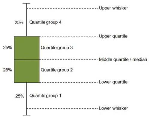
Since any form of transportation mainly depends upon the Climatic conditions, the corresponding weather information such as Temperature, Humidity, Windspeed, Visibility, Dew point temperature, rainfall, and snowfall for each hour is added. The weather information is downloaded from Korea Meteorological Administration. The processed data consists of total count of rental bikes rented at each hour with date/time variable and Weather information. Figure 2. Shows the whole process involved in data preparation. Table 1 shows the list of parameters or variables or features and its corresponding Abbreviation, Type (Continuous or categorical) and Measurement for Seoul Bike. Boxplot is a standard way of presenting the data distribution. And, it is used to see how tightly the data is grouped and to visualize the skewness in the data. As seen from Figure 3, A boxplot is composed of Lower whisker, upper whisker, lower quartile, upper quartile and middle quartile (median). Using these four quartiles groupings within the data are made. Each group has 25% of data. The middle quartile (median) represents the midpoint of the data, and it is represented by the line, which divides the box into two parts. The green box denotes the 50% of middle values in each data field considered. This range of values from lower to upper quartile limit is known as inner quartile range. 75% of values falls below the upper quartile and 25% falls above it. And, the values above the upper whisker are considered as outliers. The first step is to find the median, and all the data are grouped and displayed as box plot. In this study, a box plot-based visualization is utilized to study the data better.

Table 1. Seoul Bike data variables and description.

Parameters/Features	Abbreviation	Type	Measurement
Date	Date	Year-month-day	2017-Dec-2017 to 2018-Dec-2018
Rented Bicycle count	Count	Continuous	0,1,2,3 … .3556
Hour	Hour	Continuous	0,1,2,3 … .23
Temperature	Temp	Continuous	°C
Humidity	Hum	Continuous	%
Windspeed	Wind	Continuous	m/s
Visibility	Visb	Continuous	10 m
Dew point temperature	Dew	Continuous	°C
Solar radiation	Solar	Continuous	MJ/m2
Rainfall	Rain	Continuous	Mm
Snowfall	Snow	Continuous	Cm
Holiday	Holiday	Categorical	Holiday, Workday
Functional Day	Fday	Categorical	NoFunc, Func
Week status	Wstatus	Categorical	Weekday (Wday), Weekend (Wend)
Day of the week	Dweek	Categorical	Sunday, Monday … . Saturday
Seasons	Season	Categorical	Spring, Summer, Autumn, Winter

Figure 2. Dataset creation.

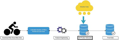
Figure 3. Boxplot details.

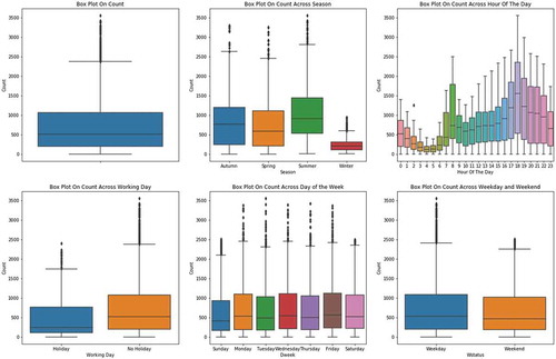
Figure 4 presents boxplots of rental bike count and rental bike count across four seasons, hour of the day, working day, day of the week and week status. Box plot of rental bike count represents the median of data is 500 and the data contains minimal outliers and there is no need for outliers removal. The boxplot across different seasons represents that the rental bike use is very less during winter season and high during the summer season. This shows the effect of weather conditions in rental bike use. The boxplot across the hour of the day represents the rental bike usage is high during hour 18 and less during hour 4. As seen from this box plot the rental bike use has a strong time component associated with it. The rental bike use is high during the working day or No holiday compared to holidays, which implies the working days influence on the rental bike usage. This may be because people use rental bikes in a regular way for their work commute. The boxplot across day of the week represents the rental bike count is slightly higher during the weekdays, and this can be witnessed in the boxplot across weekday and weekend. These relations across different time components are used to predict the rental bike count at each hour more effectively.

Figure 4. Boxplots for Rental Bike data.

The final consolidated rental bike data are partitioned into two namely, training set for building the regression and testing set for assessing the model performance by using the data partition function generated by CARET package. Usually, larger part of data is needed to teach the models and so the 75% of the final data is utilized for model training and the remaining 25% of the data is used for testing purpose. The dimensions of training and testing set for Seoul Bike data shown in Table 2.

Table 2. Seoul Bike training and testing dataset.

Dataset	Number of observed values
Training set	6571 and 16 variables
Testing set	2189 and 16 variables

To validate the performance of proposed rule-based model in bike sharing demand domain another data from Capital Bikeshare program is utilized. The Capital Bikeshare program data variables and description are given in Table 3. The data set is downloaded from Kaggle website (KAGGLE BIKE SHARING DEMAND). The training data of this competition is used in this study. Week status and Day of the week are extracted from the date and timestamp. The training data of this competition were split in to training set and testing set (See Table 4)

Table 3. Capital Bikeshare program data variables and description.

Parameters/Features	Abbreviation	Type	Measurement
Date and Time	Hourly Date and timestamp	Year-month-day	2017-Dec-2017 to 2018-Dec-2018
Number of total rentals	Count	Continuous	1,2,3 … .970
Hour	Hour	Continuous	0,1,2,3 … .23
Temperature	Temp	Continuous	°C
“feels like” temperature	Atemp	Continuous	°C
Relative Humidity	Hum	Continuous	%
Windspeed	Wind	Continuous	m/s
Seasons	Season	Categorical	Spring, Summer, Fall, Winter
Holiday	Holiday	Categorical	Holiday, NHoliday
Workingday	Work	Categorical	Work, Nwork
Weather	Weather	Categorical	Clear, Cloudy, Rain, Snow
Week status	Wstatus	Categorical	Weekday (Wday), Weekend (Wend)
Day of the week	Dweek	Categorical	Sunday, Monday … . Saturday

Table 4. Capital Bikeshare program training and testing dataset.

Dataset	Number of observed values
Training set	8166 and 11 variables
Testing set	2720 and 11 variables

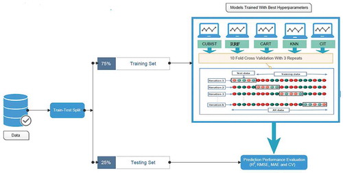
So, both the datasets are split into training and testing sets and trained with five models using 10-fold cross validation repeated thrice and their corresponding prediction performance is calculated using R², RMSE, MAE and CV. Figure 5 summarizes the total procedure involved in calculating the prediction performance in rental bike sharing demand for two datasets.

Figure 5. Illustration of total procedure.

Model development

All the models must be fine tuned with their best hyperparameters to prevent overfitting. A grid search method with repeated cross-validation (CV) was used to find the best hyperparameters. The grid search recommends parameter setting by placing all configurable grids in the parameter space. Each axis of the grid is an algorithm parameter, and a specific combination of parameters is located at each point in the grid. The function at each point needs to be optimized. To avoid data selection bias, a most commonly used method of validation, k-fold CV with repeats (Ferlito, Adinolfi, & Graditi, 2017; Kim, 2018; Kohavi, 1995; Noi, Degener, & Kappas, 2017; Rodriguez, Perez, & Lozano, 2010; Wong, 2015; Zhou et al., 2019), was employed in the process of hyperparameters tuning. K-fold CV is a common type of CV that is extensively employed in machine learning. Although a definite/strict rule for determining the value of K does not exist, a value of K = 10 is found to be optimal in many of the researches. Therefore, a total of 10 rounds of training and validating were carried out using different partitions and the same process is repeated three times; the resultant values were averaged to denote the model performance. Thus, the original training dataset was randomly divided into 10 groups, where one-tenth of the data was selected as the testing data, and the remaining nine-tenth of the data comprises the training data. For each fold CV procedure, the regression function is established, and a predictive accuracy is obtained, the total 10 CV procedures are conducted, and the final accuracy is the mean of the previously mentioned accuracy values. And, these same processes is repeated three times. All data processing in this study was performed using R software (R Core Team, 2013).

To speed up the computation process do parallel package was used (Revolution Analytics, S, 2015).

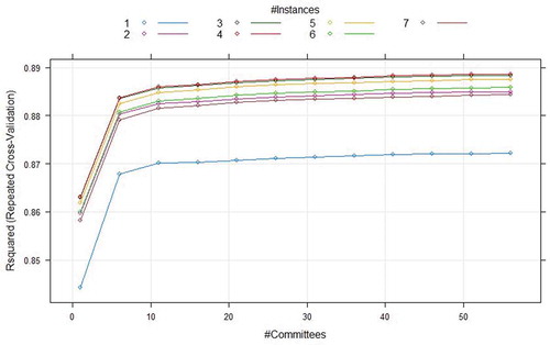
CUBIST regression model has two hyperparameters that needs to be tuned. Those are committees and neighbours. These two parameters provide maximum effect on the performance of the model. The optimal hyperparameter committees are chosen in the range of (0–50) for Seoul Bike and (0–60) for Capital Bikeshare program data. The optimal hyperparameter neighbours are selected in the scope of (1,3,5,7) for Seoul Bike and (1,2,3,4,5,6,7) for Capital Bikeshare program data. R-squared (R²) value is chosen as the measure to hyperparameter optimization. The combination of hyperparameters resulting in highest R-squared (R²) value is chosen as the best hyperparameters for each of the regression models considered. Figure 6 shows the grid search profile for Seoul Bike data and the optimal hyperparameter for Seoul Bike is found to be 41 for committees and 3 for neighbours. Figure 7 shows grid search results for Capital Bikeshare program data and the optimal hyperparameter for Capital Bikeshare program is found to be 56 for committees and 4 for neighbours.

Figure 6. Grid search results for CUBIST model using Seoul bike data.

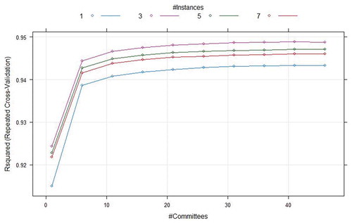
Figure 7. Grid search results for CUBIST model using Capital Bikeshare program data.

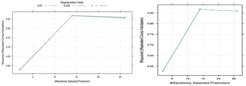
RRF has two hyperparameters Randomly selected predictors (mtry) and Regularization value (CoefReg). Since many researches proved that selecting half of the predictors is the best value for the mtry. Here in both of the datasets mtry value of 14 is chosen. The optimal value of CoefReg was found to be 0.505 for both data. Figures 8 and 9 show the grid search profiles for Seoul bike data and Capital Bikeshare program data, respectively.

Figure 8. Grid search results for RRF model using Seoul bike data.

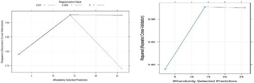
Figure 9. Grid search results for RRF model using Capital Bikeshare program data.

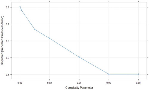
CART is a decision tree model and a condition parameter is needed to stop the growth of the tree. In this research, the complexity parameter (cp) is used as the stopping condition. The optimal hyperparameter cp is chosen in the range of {0.0001,0.001,0.01,0.1,0.2,0.4,0.6,0.8} for both of the data considered and the optimal value of cp is found to be 0.0001 for both data. The results of CART grid search for Seoul Data and Capital Bikeshare program data is displayed in Figures 10 and 11, respectively.

Figure 10. Grid search results for CART model using Seoul bike data.

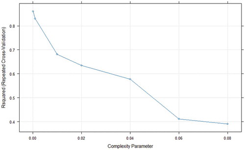
Figure 11. Grid search results for CART model using Capital Bikeshare program data.

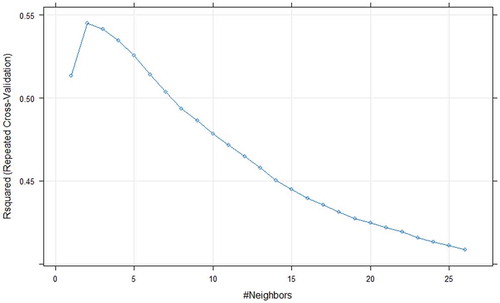
In case of KNN, the hyperparameter called number of neighbours (k) needs to be optimized. A k value search is done in the range of (0–28) for both dataset and the optimal value of k is 3 for Seoul Bike data and 2 for Capital Bikeshare program data. The results show that optimal k value found in the grid search yielded highest R-squared (R²) value (Figures 12 and 13).

Figure 12. Grid search results for KNN model using Seoul bike data.

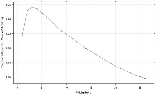
Figure 13. Grid search results for KNN model using Capital Bikeshare program data.

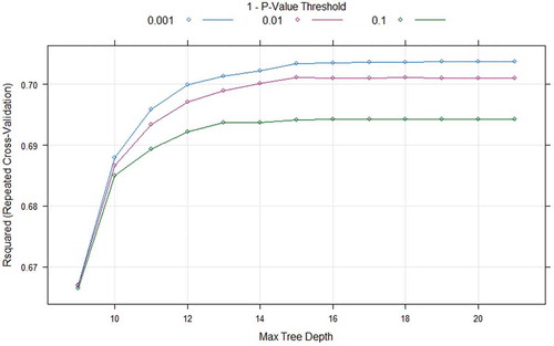
CIT model has two hyperparameters namely 1-P-value threshold (mincriterion) and Maximum tree depth(maxdepth). These parameters are used to stop the growth of the tree which are rule based. For both datasets, the hyperparameter mincriterion was searched in the scope of (0.1,0.01, 0.001) and hyperparameter maxdepth was searched in the range of (1–21). The optimal hyperparameters for mincriterion and maxdepth is 0.01 and 19 for Seoul Bike data respectively and the results are shown in Figure 14. The optimal hyperparameters for mincriterion and maxdepth is 0.001 and 21 for Capital Bikeshare program data, respectively, and the grid search output is shown in Figure 15.

Figure 14. Grid search results for CIT model using Seoul bike data.

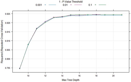
Figure 15. Grid search results for CIT model using Capital Bikeshare program data.

After training the models with their best hyperparameters, the performance of each of the regression models were evaluated using the testing set with R², RMSE, MAE and CV.

Results and discussion

Table 5 presents the developed models performance in both training set and testing sets for Seoul Bike data. The model which provide highest R² values and lowest RMSE, MAE and CV is the best one. As can be seen that CUBIST and RRF yields best results in the training set but CUBIST performance was slightly higher than RRF in the testing set. Since testing set is considered as the final performance criteria for any regression model, in this case CUBIST model has the best performance than other regression models. KNN has the worst performance compared to other prediction models. Since RF is an ensemble of numerous CART, the performance of RF is higher than CART. This proves that ensemble strategies applied on RF model makes it to perform better than CART.

Table 5. Models performance for Seoul Bike data.

			Training			Testing
Models	Hyperparameter	R^2	RMSE	MAE	CV	R^2	RMSE	MAE	CV
CUBIST	committees = 41 neighbours = 3	0.98	70.76	40.59	10.04	0.95	139.64	78.45	19.81
RRF	mtry = 14 coefReg = 0.505	0.98	75.83	44.80	10.76	0.93	164.85	99.05	23.39
CART	cp = 0.0001	0.92	177.00	113.45	25.12	0.87	228.94	141.37	32.49
KNN	k = 3	0.89	213.11	128.74	30.24	0.77	299.88	188.94	42.55
CIT	maxdepth = 19 mincriterion = 0.01	0.88	214.52	127.29	30.44	0.83	257.13	155.30	36.49

Table 6 presents the performance of the developed models in both training set and testing set for Capital Bikeshare program data. As can be seen that, in this data also CUBIST and RRF performance was quite equal in the training set but in the testing set CUBIST model performs the best. In this data also KNN model performance was not good. It can be seen from Tables 5 and 6 that in both bike sharing data CUBIST model performs the best followed by RRF. Additionally the order of performance of the regression models are also same.

Table 6. Models performance for Capital Bikeshare program.

			Training			Testing
Models	Hyperparameter	R^2	RMSE	MAE	CV	R^2	RMSE	MAE	CV
CUBIST	committees = 56 neighbours = 4	0.95	36.76	24.31	19.16	0.89	58.83	38.47	30.84
RRF	mtry = 14 coefReg = 0.505	0.96	31.80	20.88	16.57	0.86	65.41	43.46	34.29
CART	cp = 0.0001	0.87	64.04	43.03	33.38	0.80	79.91	52.58	41.89
KNN	k = 2	0.86	67.56	42.45	35.21	0.55	119.49	76.99	62.64
CIT	maxdepth = 21 mincriterion = 0.001	0.75	89.65	56.42	46.72	0.67	101.90	65.01	53.42

Relative variable importance for Seoul Bike and Capital Bikeshare program data using CUBIST, RRF, CART, KNN and CIT are shown in Figures (Figures 16 and 17). The Linear combination of rule conditions utilization by the model is used to measure the relative variable importance of CUBIST model. Residual sum of the squares is used to measure the variable importance for RRF model. CART puts track of surrogate splits in the process of tree growth and a variable contribution in prediction is not determined only by primary splits. So, the contribution of a variable in each of the split used to measure the variable importance for CART model. In case of KNN, the most chosen variable for neighbours in each new point prediction is used to measure the variable importance for KNN. Principle of Permutation in error value decrease is used to measure the CIT Variable importance.

Figure 16. Seoul bike data variable importance for CUBIST, RRF, CART, KNN and CIT.

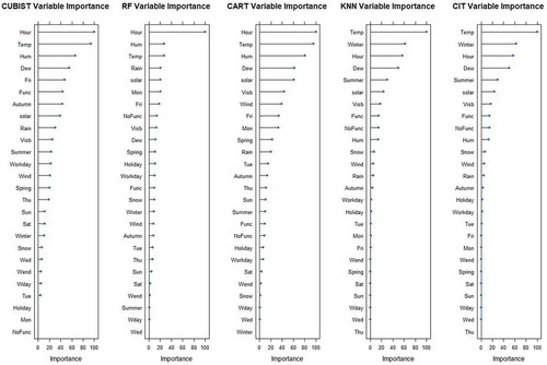
Figure 17. Capital Bikeshare program data variable importance for CUBIST, RRF, CART, KNN and CIT.

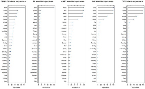
Variable importance analysis is useful for analysing the most influential features for each of the model. This analysis is useful for identifying the effect of variables considered for the developed models and for better studying the model. As can be seen from Figure 16, Hour or Temp are the most influential variable for the Seoul Bike data since these variables are ranked among top five most influential variables by all the predictive models developed. In case of Capital Bikeshare program data also Hour, Temp, aTemp and Humid variables are the most influential variables and these variables are consistently ranked in the Top 6 positions by the regression models (Figure 17). These analyses show the importance of Weather data variables, Temperature and Hour of the day is the most influential variable for rental bike sharing demand prediction.

Conclusion

This study focussed on predicting the bike sharing demand using two Bike datasets (Seoul Bike and Capital Bikeshare program). The results show that CUBIST algorithm improve the R², RMSE, MAE and CV compared to RRF, CART, KNN and CIT models in both of the datasets. This shows that CUBIST algorithm can be used as an effective tool for bike sharing demand prediction. Analysis on Variable importance was done to identify the hidden relationships between the variables. For all the models, Temperature or Hour was ranked as the most influential variable to predict the rental bike demand at each hour. This study identified the curious relationships among the variables. This study contributes to existing literature in many ways. It contributes to the research on empirical modelling-based hourly rental bike demand prediction. CUBIST belongs to the category of rule-based learning, an advance approach of empirical modelling for enhancing the performance of existing learning algorithms. While adopting CUBIST in bike sharing demand prediction and in meanwhile comparing its performance in prediction with other existing conventional algorithms i.e. RRF, CART, KNN and CIT, this paper demonstrates the superiority of CUBIST and the feasibility of rule-based learning in hourly rental bike demand prediction. These findings provide a new option for researchers to predict hourly rental bike sharing demand and enrich the library of algorithms of empirical modelling-based hourly rental bike demand prediction. Future work will focus on district wise rental bike demand prediction by considering seasonal changes.

Disclosure statement

No potential conflict of interest was reported by the authors.

References

- Altman, N.S. (1992). An introduction to kernel and nearest-neighbor nonparametric regression. The American Statistician, 46(3), 175–185.
- Barnes, G., & Krizek, K. (2005). Estimating bicycling demand. Transportation Research Record, 1939(1), 45–51. doi:10.1177/0361198105193900106
- Borgnat, P., Abry, P., Flandrin, P., & Rouquier, J.-B. (2009). Studying Lyon’s Vélo’V: A statistical cyclic model. European Conference on Complex Systems, University of Warwick in UK (vol. 2009).
- Breiman, L. (2001). Random forests. Machine Learning, 45, 5–32. doi:10.1023/A:1010933404324
- Breiman, L. (2017). Classification and regression trees. Routledge, Taylor and Francis, FL.
- Chen, T. (2003). A fuzzy back propagation network for output time prediction in a wafer fab. Applied Soft Computing, 2(3), 211–222. doi:10.1016/S1568-4946(02)00066-2
- Chen, T. (2007). An intelligent hybrid system for wafer lot output time prediction. Advanced Engineering Informatics, 21(1), 55–65. doi:10.1016/j.aei.2006.10.002
- Chen, X., & Ishwaran, H. (2012). Random forests for genomic data analysis. Genomics, 99(6), 323–329. doi:10.1016/j.ygeno.2012.04.003
- Corcoran, J., Li, T., Rohde, D., Charles-Edwards, E., & Mateo-Babiano, D. (2014). Spatio-temporal patterns of a public bicycle sharing program: The effect of weather and calendar events. Journal of Transport Geography, 41, 292–305. doi:10.1016/j.jtrangeo.2014.09.003
- DeMaio, P. (2009). Bike-sharing: History, impacts, models of provision, and future. Journal of Public Transportation, 12(4), 3.
- Deng, H., & Runger, G. (2013). Gene selection with guided regularized random forest. Pattern Recognition, 46(12), 3483–3489. doi:10.1016/j.patcog.2013.05.018
- El-Assi, W., Mahmoud, M.S., & Habib, K.N. (2017). Effects of built environment and weather on bike sharing demand: A station level analysis of commercial bike sharing in Toronto. Transportation, 44(3), 589–613. doi:10.1007/s11116-015-9669-z
- Erdoğan, G., Battarra, M., & Calvo, R.W. (2015). An exact algorithm for the static rebalancing problem arising in bicycle sharing systems. European Journal of Operational Research, 245(3), 667–679. doi:10.1016/j.ejor.2015.03.043
- Feng, C., Hillston, J., & Reijsbergen, D. (2017). Moment-based availability prediction for bike-sharing systems. Performance Evaluation, 117, 58–74. doi:10.1016/j.peva.2017.09.004
- Ferlito, S., Adinolfi, G., & Graditi, G. (2017). Comparative analysis of data-driven methods online and offline trained to the forecasting of grid-connected photovoltaic plant production. Applied Energy, 205, 116–129.
- Fishman, E. (2016). Bikeshare: A review of recent literature. Transport Reviews, 36(1), 92–113. doi:10.1080/01441647.2015.1033036
- Gao, X., & Lee, G.M. (2019). Moment-based rental prediction for bicycle-sharing transportation systems using a hybrid genetic algorithm and machine learning. Computers & Industrial Engineering, 128, 60–69.
- García-Palomares, J.C., Gutiérrez, J., & Latorre, M. (2012). Optimizing the location of stations in bike-sharing programs: A GIS approach. Applied Geography, 35(1–2), 235–246. doi:10.1016/j.apgeog.2012.07.002
- Gast, N., Massonnet, G., Reijsbergen, D., & Tribastone, M. (2015). Probabilistic forecasts of bike-sharing systems for journey planning. Proceedings of the 24th ACM international on conference on information and knowledge management held at Melbourne, Australia (pp. 703–712). ACM.
- Hothorn, T., Hornik, K., & Zeileis, A. (2006). Unbiased recursive partitioning: A conditional inference framework. Journal of Computational and Graphical Statistics, 15(3), 651–674. doi:10.1198/106186006X133933
- Kadri, A.A., Kacem, I., & Labadi, K. (2016). A branch-and-bound algorithm for solving the static rebalancing problem in bicycle-sharing systems. Computers & Industrial Engineering, 95, 41–52. doi:10.1016/j.cie.2016.02.002
- KAGGLE BIKE SHARING DEMAND (2014). Retrieved from https://www.kaggle.com/c/bike-sharing-demand/overview
- Kaltenbrunner, A., Meza, R., Grivolla, J., Codina, J., & Banchs, R. (2010). Urban cycles and mobility patterns: Exploring and predicting trends in a bicycle-based public transport system. Pervasive and Mobile Computing, 6(4), 455–466. doi:10.1016/j.pmcj.2010.07.002
- Kim, K. (2018). Investigation on the effects of weather and calendar events on bike-sharing according to the trip patterns of bike rentals of stations. Journal of Transport Geography, 66, 309–320. doi:10.1016/j.jtrangeo.2018.01.001
- Kohavi, R. (1995, August 20–25). A study of cross-validation and bootstrap for accuracy estimation and model selection. Proceedings of the International Joint Conference on Artificial Intelligence, Montreal, QC (pp. 1137–1145).
- Kuhn, M., & Johnson, K. (2013). Applied predictive modeling. New York, NY: Springer.
- Kuhn, M., Weston, S., Keefer, C., Coulter, N., & Quinlan, R. (2014). Cubist: Rule-and instance-based regression modeling, R package version 0.0.18. Vienna, Austria: CRAN.
- Meng, L.D. (2011). Implementing bike-sharing systems. Proceedings of the Institution of Civil Engineers, 164(2), 89.
- Noi, P., Degener, J., & Kappas, M. (2017). Comparison of multiple linear regression, cubist regression, and randomforest algorithms to estimate daily air surface temperature from dynamic combinations of MODIS LSTdata. Remote Sensing, 9, 398. doi:10.3390/rs9050398
- Quinlan, R. (1992, November 16–18). Learning with continuous classes. Proceedings of the 5th Australian Joint Conference on Artificial Intelligence, Hobart, Australia (pp. 343–348).
- Quinlan, R. (1993, June 27–29). Combining instance based and model based learning. Proceedings of the Tenth International Conference on Machine Learning, Amherst, MA (pp. 236–243).
- R Core Team. (2013). R: A language and environment for statistical computing. Vienna, Austria: R Foundation for Statistical Computing. ISBN 3-900051-07-0. Retrieved from https://www.R-project.org/
- Raviv, T., & Kolka, O. (2013). Optimal inventory management of a bike-sharing station. Iie Transactions, 45(10), 1077–1093. doi:10.1080/0740817X.2013.770186
- Revolution Analytics, S. (2015). Weston, doParallel: Foreach Parallel Adaptor for the ‘parallel’ Package. Retrieved from https://mran.revolutionanalytics.com/snapshot/2016-01-01/web/packages/doParallel/doParallel.pdf
- Rodriguez, J.D., Perez, A., & Lozano, J.A. (2010). Sensitivity analysis of k-fold cross validation in prediction error estimation. IEEE Transactions on Pattern Analysis and Machine Intelligence, 32, 569–575. doi:10.1109/TPAMI.2009.187
- Russell, S.J., & Norvig, P. (2016). Artificial intelligence: A modern approach. Malaysia: Pearson Education Limited.
- Schuijbroek, J., Hampshire, R.C., & Van Hoeve, W.-J. (2017). Inventory rebalancing and vehicle routing in bike sharing systems. European Journal of Operational Research, 257(3), 992–1004.
- SEOUL OPEN DATA PLAZA. (2017-2018) Retrieved from http://data.seoul.go.kr/
- Shaheen, S.A., Guzman, S., & Zhang, H. (2010). Bikesharing in Europe, the Americas, and Asia: Past, present, and future. Transportation Research Record, 2143(1), 159–167. doi:10.3141/2143-20
- Shaheen, S.A., Martin, E.W., Cohen, A.P., Chan, N.D., & Pogodzinski, M. (2014). Public Bikesharing in North America during a period of rapid expansion: Understanding business models. Industry Trends & User Impacts, MTI Report, San Jose State University, 12–29.
- Strobl, C., Boulesteix, A.-L., Zeileis, A., & Hothorn, T. (2007). Bias in random forest variable importance measures: Illustrations, sources and a solution. BMC Bioinformatics, 8(1), 25. doi:10.1186/1471-2105-8-25
- Tirkel, I. (2011). Cycle time prediction in wafer fabrication line by applying data mining methods. 2011 IEEE/SEMI Advanced Semiconductor Manufacturing Conference, Saratoga Springs, NY (pp. 1–5). IEEE.
- Vogel, P., & Mattfeld, D.C. (2011). Strategic and operational planning of bike-sharing systems by data mining–A case study. International Conference on Computational Logistics (pp. 127–141). Springer: Berlin, Heidelberg.
- Wang, Y., & Witten, I. (1996, April 23–25). Inducing model trees for continuous classes. Proceedings of the Ninth European Conference on Machine Learning, Prague, Czech Republic (pp. 128–137).
- Wolpert, D.H., & Macready, W.G. (1997). No free lunch theorems for optimization. IEEE Transactions on Evolutionary Computation, 1(1), 67–82. doi:10.1109/4235.585893
- Wong, T.T. (2015). Performance evaluation of classification algorithms by k-fold and leave-one-out cross validation. Pattern Recognit, 48, 2839–2846. doi:10.1016/j.patcog.2015.03.009
- Zhou, J., Li, E., Wang, M., Chen, X., Shi, X., & Jiang, L. (2019). Feasibility of stochastic gradient boosting approach for evaluating seismic liquefaction potential based on SPT and CPT Case Histories. Journal of Performance of Constructed Facilities, 33, 04019024.