MODIS-based land surface temperature for climate variability and change research: the tale of a typical semi-arid to arid environment

ABSTRACT

This study aims to (1) determine the seasonalities and spatial and temporal rates of change of MODIS-based daytime and nighttime land surface temperature (LST) for the last 19 years from 2000 to 2018 and (2) investigate whether these rates are induced by natural (represented by elevation) or anthropogenic (represented by population counts) forcing. The study area is Jordan – a typical Middle Eastern semi-arid to arid country. Time-series additive seasonal decomposition and simple linear regression produced the following results. (1) For both daytime and nighttime the highest LST values were observed in June while the lowest LST values were observed in December. (2) No significant linear rates of change of LST were noticed in daytime, while significant linear rates of increase of LST, which varied from 0.041°C/year to 0.119°C/year, were observed in nighttime in about one-third of the area of the country mainly in the western parts. (3) The significant linear rates of increase of nighttime LST increased significantly by 0.005°C/year for every 1,000 m increase in elevation and by 0.003°C/year for every 1,000 people increase in population counts. (4) Both natural and anthropogenic factors affected LST in nighttime; however, anthropogenic factors seemed to be more important than natural factors.

KEYWORDS:

• MODIS
• land surface temperature
• climate variability and change
• ASTER Global Digital Elevation Model
• Global Human Settlement Population Grid
• Jordan

Introduction

Climate is dynamic; it is varying and changing at all spatial and temporal scales. Climate variabilities and changes have happened in the past and will continue to happen in the future. The major current concern stems not from these variabilities and changes but from their rates and possible connection to human activities (IPCC, 2013).

One of the most important climatic elements is land surface air temperature (LSAT), which is the temperature of air adjacent to the earth surface. It is usually measured at 1.2–1.8 m above the earth surface by employing common weather stations distributed across a certain area (Christopherson & Birkeland, 2018). However, measurements of LSAT using weather stations represent only discrete point measurements at specific locations, which require applying further interpolation and extrapolation techniques in order to fill in gaps in places where there are no direct measurements. Due to the paucity of weather stations in many areas in the world, especially in developing countries, and because the accuracies of these techniques decrease, especially in areas that have certain characteristics such as complex terrain, complementary methods should be used (Mutiibwa, Strachan, & Albright, 2015).

Land surface temperature (LST) is the radiative skin temperature of land surface derived from solar radiation. It is a measure of how hot the earth surface would feel to touch in a particular location (https://sentinel.esa.int/web/sentinel/user-guides/sentinel-3-slstr/overview/geophysical-measurements/land-surface-temperature, accessed 29 October 2018). Despite the facts that the physical principles of LSAT and LST are different and the relationship between them is complex (Mutiibwa et al., 2015; Noi, Kappas, & Degener, 2016), multiple studies indicated the presence of significant positive correlation between them (Gallo, Hale, Tarpley, & Yu, 2011; Kawashima, Ishida, Minomura, & Miwa, 2000; Lin et al., 2016; Nichole, 1996; Schlink, Franck, & Großmann, 2012); a reality that makes LST a candidate for being possible proxy and advocate for LSAT.

LST is a complex variable and is impacted by many factors that force it to change rapidly spatially and temporally (Bertoldi et al., 2010; Jaber, 2018; Peng, Zhoua, Wena, Xuea, & Dong, 2017; Xiao et al., 2008). These constraints make the quantification of LST using direct ground measurements impractical. An alternative is to use satellite-based remote sensing sensors, which have thermal infrared (TIR) bands to obtain indirect, cost-effective, continuous, and spatially averaged LST data over large areas on a repetitive basis (Li et al., 2013).

Launched in 1999, MODIS instrument onboard Terra satellite provides global free-of-charge LST data that represent both daytime land surface temperature (LSTD) at 10:30 am local time, and nighttime land surface temperature (LSTN) at 10:30 pm local time (https://modis.gsfc.nasa.gov/data/dataprod/mod11.php, accessed 29 October 2018). The instrument makes a compromise between reasonable spatial resolution and reasonable temporal resolution, which makes it suitable for large areas. The latest release of MODIS LST Products is named Collection 6 (C6) or Version 6 (V6). This collection is available to the public since 2016. Validation of LST products derived from C6 MODIS thermal infrared data using in situ measurements was achieved over a widely distributed set of locations and time periods (Duan, Li, Wu, et al.,  2018; Duan et al., 2019; Lu, Zhang, Wang, & Zhou, 2018; Wan, 2014). This collection incorporates improvements in retrieval algorithms and hence is more accurate than its predecessor Collection 5 (C5) LST products specifically over semi-arid and arid regions and also over bare soil areas (Sharifnezhadazizi, Norouzi, Prakash, Beale, & Khanbilvardi, 2019). Therefore, C6 MODIS LST products are ready to use in scientific applications.

Accordingly, this study aims at determining the seasonalities and spatial and temporal rates of change of MODIS-based LST data and exploring whether these rates differ between daytime and nighttime in Jordan – a typical Middle Eastern semi-arid to arid country. Interestingly, the literature in this specific area of application is not at the desired level of ambitions and aspirations (Eleftheriou et al., 2018; Luintel, Weiqiang, Yaoming, Binbin, & Sunil, 2019; Mao et al., 2017; Sun, Wan, Imbery, Lotz, & King, 2015; Zhao et al., 2019), which makes this type of studies important in order to fill in this serious scientific gap. This study also aims at investigating whether the discerned daytime and nighttime spatial and temporal rates of change of MODIS-based LST in the study area are natural or anthropogenic. Hence, two variables were subjected to investigation: the first represents the natural factors, which is elevation, and the second represents the anthropogenic factors, which is population counts. Elevation (Bandopadhyay, 2016; Beniston, Diaz, & Bradley, 1997; Palazzi, Mortarini, Terzago, & Hardenberg, 2019; Rangwala & Miller, 2012; Revadekar et al., 2013) and population dynamics (Dodman, 2009; Je, 2010; Jiang & Hardee, 2009; Zlotnik, 2009) play important, diverse, and complex roles in climate variability and change. Although various attempts tried to explore the determinant factors controlling the spatial and temporal behavior of LST (Bertoldi et al., 2010; Jaber, 2018; Peng et al., 2017; Xiao et al., 2008), they lack the desired consideration and, therefore, more studies are demanded in order to expand and nourish the current understanding and knowledge about the spatial and temporal behavior of LST.

This study represents a direct response to the demands put by the Intergovernmental Panel on Climate Change (IPCC) for urgently developing a remote sensing-based LST data for climate variability and change research in order to improve the limitations of weather-based conventional LSAT observations (IPCC, 2013). The results of this study will help to reveal the usefulness of MODIS-based LST data for enriching the literature and providing supporting evidence for climate variability and change research locally and globally.

Study area and data set

The study area is the entire territories of the Hashemite Kingdom of Jordan, which covers an area of about 88,780 km² (Figure 1). It lies between latitudes 29°N and 34°N and longitudes 34°E and 40°E. According to the population clock, the country hosts about 10,415,544 inhabitants as of 1 June 2019 (http://dosweb.dos.gov.jo/, accessed 1 June 2019). More than 42% of the population of the country settles in Amman Governorate, which encapsulates the capital Amman City. Jordan climate is semi-arid to arid; the northern and western parts have a Mediterranean climate with hot dry summers and cool wet winters while the southern and eastern parts are arid with hot dry summers and cool dry winters (IUCN, 2014).

Figure 1. Location, elevation, and population distribution maps of the Hashemite Kingdom of Jordan

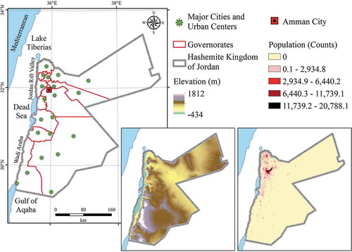
Elevation data for Jordan were obtained from the ASTER Global Digital Elevation Model (GDEM) Version 2 product. This product provides elevation values in meters configured on a 1 arc-second grid (https://asterweb.jpl.nasa.gov/gdem.asp, accessed 18 February 2019). After downloading the data for Jordan from the LP DAAC website (https://lpdaac.usgs.gov/, accessed 18 February 2019), it was re-projected to the Jordan Transverse Mercator (JTM) coordinate system (Figure 1). Jordan is divided into three main regions. A range of mountains with elevations reach 1,812 m above mean sea level, which form the highlands, and run from north to south. East of the mountains, the land slopes gently to the east to form the eastern deserts with mean elevations of 750 m above mean sea level. West of the mountains, the land slopes steeply towards the Jordan Rift Valley in the north and Dead Sea (the lowest point on earth) in the middle with elevations reach −434 m below mean sea level and Wadi Araba and Gulf of Aqaba in the south.

Population count data for Jordan were obtained from the Global Human Settlement (GHS) Population Grid (LDS) product (Martino, Michele, Alice, & Thomas, 2016). This product is multi-temporal and depicts the distribution and density of population in the past 1975, 1990, 2000, and 2014 expressed as the number of people per pixel configured on a 1,000 m grid. After downloading the data for Jordan from the European Commission website (https://ghsl.jrc.ec.europa.eu/data.php, accessed 15 February 2019), it was re-projected to the JTM coordinate system (Figure 1). In Jordan, the pixels have values that vary from zero to 20,788 people with a mean of 84 people. About 94% of the total area of the country has zero people per pixel values. Pixels that have non-zero values exist mainly in the capital city in addition to the major cities and urban centers along the highlands and also west of the highlands especially in the north and the middle.

LST data for Jordan were extracted from the MODIS/Terra LST/E Monthly L3 Global 0.05°CMG (MOD11C3) Version 006 product. This product provides monthly daytime and nighttime per-pixel LST values in Kelvin configured on a 0.05° grid (https://modis.gsfc.nasa.gov/data/dataprod/mod11.php, accessed 20 February 2019). After downloading the data for Jordan for the period from February 2000 to December 2018 from the LP DAAC website (https://lpdaac.usgs.gov/, accessed 20 February 2019), they were re-projected to the JTM coordinate system and converted into degree Celsius (°C). The result was the production of 227 maps showing the spatial distribution of monthly LSTD and 227 maps showing the spatial distribution of monthly LSTN for Jordan. Time-series scatterplots were constructed for the means of the 227 maps showing the spatial distribution of monthly LSTD and the means of the 227 maps showing the spatial distribution of monthly LSTN. The means of monthly LSTD varied from 13.8°C to 50.6°C with a mean of 35.1°C (Figure 2). The means of monthly LSTN varied from 0.2°C to 27.0°C with a mean of 14.8°C (Figure 3).

Figure 2. The results of applying time-series additive seasonal decomposition on the means of monthly LSTD

Figure 3. The results of applying time-series additive seasonal decomposition on the means of monthly LSTN

Methodology

Two paths, which complement and accentuate each other and provide different levels of information, were followed in order to achieve the first goal of this study and determine the seasonalities of LSTD and LSTN and calculate their spatial and temporal rates of change. In the first path, time-series additive seasonal decomposition (Hyndman & Athanasopoulos, 2018) was applied in order to decompose the time-series showing the means of monthly LSTD for Jordan for the period from February 2000 to December 2018 into trend-cycle, seasonal, and irregular components (Equation 1(1) $Y=TC+S+I$(1) ) based on sampling interval of 1 month and length of seasonality of 12 months. The trend-cycle component represents the general long-term trend and long-term cyclical variations around the trend that are not of a fixed period. The seasonal component represents the short-term cyclical variations around the trend that are of the fixed period influenced by seasonal factors. Seasonality can be represented in the form of seasonal indices for each month scaled so that an average month equals zero. The irregular component represents the residual random noise.

(1) $Y=TC+S+I$(1)

where $Y$ is the observed monthly means of LSTD or monthly means of LSTN; $TC$ is the trend-cycle component; $S$ is the seasonal component; $I$ is the irregular component.

Then, simple linear regression using the method of least squares (Hansen, Pereyra, & Scherer, 2013) was applied on the extracted trend-cycle component in order to calculate its monthly linear rate of change represented by the regression coefficient (Equation 2(2) $b_1=\frac{\sum \left(t_i-\bar{t}\right)\left(T{C}_i-\overline{TC}\right)}{\sum {\left(t_i-\bar{t}\right)}^2}$(2) ).

(2) $b_1=\frac{\sum \left(t_i-\bar{t}\right)\left(T{C}_i-\overline{TC}\right)}{\sum {\left(t_i-\bar{t}\right)}^2}$(2)

where $b_1$ is the regression coefficient which is the slope of the regression line which is the change in trend-cycle component associated with every 1-month increase (°C/month); $t_i$ is the time (month); $\bar{t}$ is the mean of time (month); $T{C}_i$ is the trend-cycle component (°C); $\overline{TC}$ is the mean of the trend-cycle component (°C).

Since the value obtained for the regression coefficient was extracted from a sample $\left(b_1\right)$ and in order to generalize it to the population $({\beta }_1)$ it must be tested to see if it is significant. This was done by constructing its confidence interval at 95% confidence level (Equations 3(3) $CI=b_1\pm \left(t_{\alpha /2}S{E}_{b_1}\right)$(3) –6(6) $b_0=\overline{TC}-b_1\bar{t}$(6) ) where the null hypothesis is $H_0:{\beta }_1=0$ (Ranstam, 2012). From a statistical point of view, when zero is a potential value for a parameter falling within its confidence interval, the parameter is set to be statistically not significant. Then, a similar analysis was repeated for LSTN.

(3) $CI=b_1\pm \left(t_{\alpha /2}S{E}_{b_1}\right)$(3)

where $CI$ is the confidence interval estimate for ${\beta }_1$ which is the population parameter estimated using the sample statistic $b_1$; $t_{\alpha /2}$ is the critical value obtained from the t-Table at confidence level α and degrees of freedom df; $S{E}_{b_1}$ is the standard error of $b_1$ and is computed using Equation 4(4) $S{E}_{b_1}=\sqrt{\frac{\sum \frac{{\left(T{C}_i-\widehat{T{C}_i}\right)}^2}{\left(n-2\right)}}{\sum {\left(t_i-\bar{t}\right)}^2}}$(4) .

(4) $S{E}_{b_1}=\sqrt{\frac{\sum \frac{{\left(T{C}_i-\widehat{T{C}_i}\right)}^2}{\left(n-2\right)}}{\sum {\left(t_i-\bar{t}\right)}^2}}$(4)

where $n$ is the sample size and equals 215; $\widehat{T{C}_i}$ is the predicted trend-cycle component and is computed using Equation 5(5) $\widehat{T{C}_i}=b_0+b_1{t}_i$(5) .

(5) $\widehat{T{C}_i}=b_0+b_1{t}_i$(5)

where $b_0$ is the intercept of the regression line which is the value of the trend-cycle component at $t=0$ and is computed using Equation 6(6) $b_0=\overline{TC}-b_1\bar{t}$(6) .

(6) $b_0=\overline{TC}-b_1\bar{t}$(6)

In the second path, a simple linear regression using the method of least squares was applied on every pixel of the 227 maps showing the spatial distribution of monthly LSTD for Jordan for the period from February 2000 to December 2018. Hence, the monthly linear rates of change for every pixel represented by the regression coefficients were calculated and presented in the form of a map. Then, the significance of the obtained regression coefficients for every pixel was tested by constructing their confidence intervals at 95% confidence level and presented in the form of a map where the null hypothesis is $H_0:{\beta }_1=0$. Equations 2(2) $b_1=\frac{\sum \left(t_i-\bar{t}\right)\left(T{C}_i-\overline{TC}\right)}{\sum {\left(t_i-\bar{t}\right)}^2}$(2) –6(6) $b_0=\overline{TC}-b_1\bar{t}$(6) as described earlier were used. Finally, a similar analysis was repeated for the 227 maps showing the spatial distribution of monthly LSTN for Jordan for the period from February 2000 to December 2018.

In order to achieve the second goal of this study and investigate whether the discerned daytime and nighttime spatial and temporal linear monthly rates of change of LST in Jordan are natural or anthropogenic, a simple linear regression using the method of least squares was applied again between the statistically significant linear monthly rates of change of LST (dependent variable) and elevation and population counts (independent variables). The significance of the obtained regression coefficients was also tested by constructing their confidence intervals at 95% confidence level where the null hypothesis is $H_0:{\beta }_1=0$ (Equations 2(2) $b_1=\frac{\sum \left(t_i-\bar{t}\right)\left(T{C}_i-\overline{TC}\right)}{\sum {\left(t_i-\bar{t}\right)}^2}$(2) –6(6) $b_0=\overline{TC}-b_1\bar{t}$(6) ). Furthermore, in order to reveal which variable is most important as determinant factor for LST, the standardized regression coefficients associated with elevation and population counts were calculated by first standardizing the dependent and independent variables by subtracting their means and dividing by their standard deviations and then repeating the simple linear regression analysis on the standardized variables and also testing the statistical significance at 95% significance level of the resulted standardized regression coefficients where the null hypothesis is $H_0:{\beta }_1=0$ as has been explained above. Standardizing regression coefficients put them on the same scale and allows their direct comparison; i.e. it rules out the impact of the differences in units of measurement of different variables. Therefore, the independent variable with the largest statistically significant absolute value for the standardized coefficient should be relatively the most important one.

Results and discussion

The methodology followed in order to achieve the goals of the present study in Jordan in the 19-year period from February 2000 to December 2018 produced the following complementary results that need further discussion.

First, time-series additive seasonal decomposition applied on the means of monthly LSTD and means of monthly LSTN data showed that for both daytime and nighttime the highest means of monthly LST values were observed in June (Figures 2 and 3) when the sun is overhead the Tropic of Cancer where the angle of incidence of solar radiation is highest in the northern Hemisphere. Likewise, the lowest means of monthly LST values were observed in December (Figures 2 and 3) when the sun is overhead the Tropic of Capricorn where the angle of incidence of solar radiation is lowest in the northern Hemisphere. This implies that LST is directly related to the intensity of solar radiation, which itself depends on the angle of incidence of solar radiation. This seasonality of LST coincides with that of LSAT in the northern Hemisphere; the astronomically summers and winters last from 21 June to 23 September and from 21 December to 20 March, respectively.

Second, the trend-cycle components for both daytime and nighttime resulted from applying time-series additive seasonal decomposition on the means of monthly LSTD and means of monthly LSTN data showed huge variability with up and down movements with no readily noticeable general linear trends of increase or decrease (Figures 2 and 3). Variations in atmospheric turbidity due to natural and anthropogenic sources in addition to clouds are likely the main causes for this observed variability. Applying simple linear regression on daytime and nighttime trend-cycle components and constructing confidence intervals at 95% confidence level for the resulted regression coefficients (Table 1) revealed that no statistically significant linear rate of change (either increase or decrease) of LST was noticed in daytime. However, the statistically significant linear rate of increase of 0.032°C/year of LST was observed in nighttime. Again, applying simple linear regression on every pixel of the 227 maps showing the spatial distribution of monthly LSTD and on every pixel of the 227 maps showing the spatial distribution of monthly LSTN and constructing confidence intervals at 95% confidence level for the resulted regression coefficients (Figures 4 and 5) showed similar and supporting results to those obtained from the first path. In addition, the results showed also the spatial distribution of the statistically significant and not significant linear rates of change in the country. In daytime, almost everywhere in the country (about 99% of the total area of Jordan), no statistically significant linear rates of change (either increase or decrease) of LST were noticed. However, in nighttime statistically significant linear rates of increase of LST were observed in about 30% of the total area of Jordan. These nighttime significant rates of increase varied from 0.041°C/year to 0.119°C/year. Nighttime significant rates of increase are likely attributed to changes in air composition due to increases in the abundances of atmospheric carbon dioxide and methane, the potent greenhouse gasses. Greenhouse gasses suppress cooling the earth surface by trapping terrestrial thermal radiation. Comparable results were reported in Nepal (Luintel et al., 2019; Zhao et al., 2019); the authors indicated that the mean annual LST and annual maximum LST in nighttime had mean change rates in the period 2000–2017 of about 0.048°C/year and 0.091°C/year, respectively. However, nighttime significant rates of increase obtained from the present study might be described as being faster than those obtained for Greece (Eleftheriou et al., 2018); the authors indicated that nighttime LST demonstrated increasing annual trends in the period 2000–2017 ranging from 4.6 × 10⁻⁵ to 3.1 × 10⁻³°C/year. It is worth mentioning that the three countries exist in different geographic locations and represent various environmental, social, and economic characteristics: Jordan is Middle-Eastern, upper-middle-income, mainly arid, comprises the lowest point on earth (Dead Sea), and according to the 2017 World Bank estimates had an increasing population growth rate of 2.6%; Nepal is South-Asian, low-income, mainly warm temperate to polar, comprises the highest point on earth (Mount Everest), and according to the 2017 World Bank estimates had an increasing population growth rate of 1.1%; Greece is European, high-income, mainly warm temperate, coastal, and according to the 2017 World Bank estimates had a decreasing population growth rate of −0.2%. Comparing these results obtained for nighttime LST, which is equivalent to nighttime minimum LSAT, from the present study to those reported for LSAT locally and globally, it can be noticed that they both behaved comparably. Hamdi, Abu-Allaban, Elshaieb, Jaber, and Momani (2009) reported significant increases in nighttime minimum LSAT at several meteorological stations throughout Jordan. Jones, New, Parker, Martin, and Rigor (1999) reported that in the last decades of the twentieth century there have been much greater increases in nighttime minimum LSAT than in daytime maximum LSAT. Abu Sada, Abu-Allaban, and Al-Malabeh (2015) published comparable values for the rate of LSAT increases for several locations at north Jordan; their findings indicated that LSAT is increasing at an annual rate of 0.02–0.06°C/year. However, the nighttime significant rates of increase obtained from the present study for LSTN might be described as being faster than those obtained for LSAT globally; according to NASA’s GISS ongoing temperature analysis, the average global temperature on earth increased by about 0.8°C since 1880 (i.e., 0.006°C/year in the last 140 years or so) and two-thirds of the warming occurred since 1975 at a rate of about 0.15–0.20°C/decade (i.e., 0.015–0.020°C/year) (https://earthobservatory.nasa.gov/world-of-change/DecadalTemp, accessed 12 June 2019).

Table 1. The results of applying simple linear regression using the method of least squares

Dependent variable	Independent variable	Coefficient	Confidence interval
Daytime trend-cycle component (°C)	Time (month)	0.000939 (°C/Month)	$-0.000032\le {\beta }_1\le 0.001911$
Nighttime trend-cycle component (°C)	Time (month)	0.002669 (°C/Month)	$0.001799\le {\beta }_1\le 0.003538$
Statistically significant linear rates of change of LSTN (°C/Month)	Elevation (m)	$4.1506\times {10}^{-7}$((°C/Month)/m)	$2.6125\times {10}^{-7}\le {\beta }_1\le 5.6887\times {10}^{-7}$
Standardized statistically significant linear rates of change of LSTN	Standardized elevation	0.167122	$0.105190\le {\beta }_1\le 0.229053$
Statistically significant linear rates of change of LSTN (°C/Month)	Population (counts)	$2.4703\times {10}^{-7}$((°C/Month)/Counts)	$2.0563\times {10}^{-7}\le {\beta }_1\le 2.8844\times {10}^{-7}$
Standardized statistically significant linear rates of change of LSTN	Standardized population	0.350961	$0.292142\le {\beta }_1\le 0.409780$

For a regression coefficient to be statistically significant, zero should not be a potential value within its confidence interval.

Figure 4. The results of applying simple linear regression using the method of least squares on every pixel of the 227 maps showing the spatial distribution of monthly LSTD and constructing confidence intervals at confidence level of 95% for the regression coefficients

Note: For a regression coefficient to be statistically significant, zero should not be a potential value within its confidence interval.

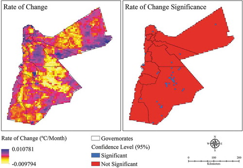
Figure 5. The results of applying simple linear regression using the method of least squares on every pixel of the 227 maps showing the spatial distribution of monthly LSTN and constructing confidence intervals at confidence level of 95% for the regression coefficients

Note: For a regression coefficient to be statistically significant, zero should not be a potential value within its confidence interval.

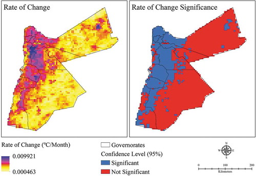
Third, applying simple linear regression between the statistically significant linear rates of increase of LSTN (dependent variable) and elevation (independent variable) (Table 1) showed that the statistically significant linear rates of increase of LSTN increased significantly by 0.005°C/year for every 1,000 m increase in elevation. The statistically significant linear rates of increase of LSTN were found mainly in the western parts of the country (Figure 5). These areas encompass the range of mountains which form the highlands in the middle and run from north to south in addition to the steeply slope lands west of the mountains towards the Jordan Rift Valley in the north and the Dead Sea in the middle and Wadi Araba and Gulf of Aqaba in the south. Elevations in these areas varied from −411 m to 1,708 m with a mean of 740 m. Elevation-dependent warming is an ongoing and active area of research; multiple studies showed that the rates of warming within mountain regions are changing at different rates than rest of the global land surface and the rates of change differ depending on elevation within a specific mountain range often with greater increases in nighttime minimum LSAT than daytime maximum LSAT (Bandopadhyay, 2016; Beniston et al., 1997; Diaz & Bradley, 1997; Giorgi, Hurrell, Marinucci, & Beniston, 1997; Liu, Cheng, Yan, & Yin, 2009; Palazzi et al., 2019; Qin, Yang, Liang, & Guo, 2009; Rangwala & Miller, 2012; Revadekar et al., 2013). Again, applying simple linear regression between the statistically significant linear rates of increase of LSTN (dependent variable) and population counts (independent variable) (Table 1) showed that the statistically significant linear rates of increase of LSTN increased significantly by 0.003°C/year for every 1,000 people increase in population counts. The statistically significant linear rates of increase of LSTN were found mainly also in the western parts of the country (Figure 5) where major cities and urban centers exist. Population counts per pixel in these areas varied from zero to 16,831 people with a mean of 233 people. It is not really understood how population dynamics affect climate variability, but it is agreed upon that population growth is one of the major driving forces of the growth in greenhouse gas emissions, which in turn induce climate variability and change (Jiang & Hardee, 2009). Multiple studies reported that 1% increase in population is generally associated with a 1% increase in carbon emissions after controlling for other variables, mainly economic growth and technology related to energy efficiency and carbon intensity (Dietz & Rosa, 1997; Shi, 2003; York, Rosa, & Dietz, 2003). It is worth mentioning that the increase in elevation in Jordan is associated with an increase in population density because eastern and southern areas, which make up more than 80% of Jordan, are mainly barren deserts that host few thousands of nomads.

Fourth, although the regular regression coefficients associated with elevation and population counts might give an impression that the annual increase in LSTN associated with every 1,000 m increase in elevation is faster than the annual increase in LSTN associated with every 1,000 people increase in population counts, by looking at the standardized regression coefficients associated with elevation and population counts (Table 1) it can be concluded that population counts are relatively more important than elevation as a determinant factor for the statistically significant linear rates of increase of nighttime LST. This might provide empirical evidence that both natural and anthropogenic variables affect LST; however, anthropogenic variables might be looked at as being precedent and superior over natural variables as determinant factors for nighttime LST. However, more studies that include other natural and anthropogenic variables are recommended. These studies should investigate the relative importance of these variables as determinant factors for LST.

Summary and conclusion

Direct measurements of LSAT using conventional weather stations at specific locations need applying interpolation and extrapolation techniques in order to fill in the gaps where there are no direct measurements. Due to limitations associated with the accuracies of these interpolation and extrapolation techniques and the paucity of weather stations in many areas in the world, especially in developing countries and areas that have certain characteristics such as deserts, forests, high mountains, in addition to highly densely populated urban areas, complementary methods should be used. Despite the fact that the physical principles of weather stations-based LSAT and satellite-based LST are different, multiple studies showed the presence of a statistically significant positive correlation between these two environmental parameters. Therefore, satellite-based LST can be regarded as being possible proxy and advocate for weather stations-based LSAT. Furthermore, for climate variability and change research, the IPCC demanded urgently developing an indirect satellite-based LST data to fill in the gaps of direct weather stations-based LSAT data. Accordingly, the present study aims to (1) determine the seasonalities and spatial and temporal rates of change of MODIS-based daytime and nighttime LST (extracted from MOD11C3 Version 006 product) for the last 19 years from February 2000 December 2018 and (2) investigate whether these rates are influenced by natural (represented by elevation data extracted from ASTER GDEM Version 2 product) or anthropogenic (represented by population counts extracted from GHS LDS product) forcing. The study area is the whole territories of the Hashemite Kingdom of Jordan, which represents a typical Middle-Eastern semi-arid to arid environment.

Applying time-series additive seasonal decomposition and simple linear regression showed that: (1) for both daytime and nighttime the highest LST values were observed in June while the lowest LST values were observed in December; (2) no significant linear rates of change of LST were noticed in daytime while significant linear rates of increase of LST, which varied from 0.041°C/year to 0.119°C/year, were observed in nighttime in about one-third of the area of the country mainly in the western parts; (3) the significant linear rates of increase of nighttime LST increased significantly by 0.005°C/year for every 1,000 m increase in elevation and by 0.003°C/year for every 1,000 people increase in population counts; and (4) both natural and anthropogenic factors affected LST in nighttime; however, anthropogenic factors seemed to be more important than natural factors.

The observations about LST obtained from the present study mimic with varying degrees of conventional weather station-based observations about LSAT obtained from other studies throughout Jordan and the world. While northwestern and western parts of Jordan enjoy Mediterranean climate with mild winter months and hot summer days, eastern and southern parts of the country are more subject to sub-Sahara type climate with very hot summer months, mild winter days, and cold winter nights. Eastern and southern Jordanian territories exist in the shadow of the mountains. In addition, they are distant from the main water body (the Mediterranean Sea) and lack nighttime clouds that play important role in controlling LST and LSAT by trapping thermal radiation, which make them subject to fast night radiation cooling.

So, what are the implications of the results obtained from this study to climate variability and change research? Well, the answer is complex and multifaceted and relies heavily on: (1) our understanding of the terms climate variability and climate change and LST and their determinant factors, (2) our understanding of the roles, which LST play in climate variability and change, (3) the advancements happened and will happen to the fields of spatial and temporal modeling specifically for developing models that can explain and predict LST accurately under different conditions, and (4) the advancements happened and will happen to the remote sensing science and technology specifically for monitoring LST accurately under different conditions. It is worth mentioning that MODIS-based LST data, which were used herein, dates back to February 2000. This 19-year time-series might be considered beneficial for climate variability research. However, as time goes on and more data are collected climate change research might also benefit from similar studies. It is well known that climate variability describes short-term fluctuations of climate while climate change describes long-term trend or continuous change of climate.

Disclosure Statement

No potential conflict of interest was reported by the authors.

References

- Abu Sada, A. , Abu-Allaban, M. , & Al-Malabeh, A. (2015). Temporal and spatial analysis of climate change at Northern Jordanian Badia. Jordan Journal of Earth and Environmental Science , 7, 87–93.
- Bandopadhyay, S. (2016). Does elevation impact local level climate change? An analysis based on fifteen years of daily diurnal data and time series forecasts. Pacific Science Review A: Natural Science and Engineering , 18, 241–253.
- Beniston, M. , Diaz, H.F. , & Bradley, R.S. (1997). Climate change at the high elevation sites: An overview. Climate Change , 36, 233–251. doi:10.1023/A:1005380714349
- Bertoldi, G. , Notarnicola, C. , Leitinger, G. , Endrizzi, S. , Zebisch, M. , Chiesa, S.D. , & Tappeiner, U. (2010). Topographical and ecohydrological controls on land surface temperature in an alpine catchment. Ecohydrology , 3, 189–204.
- Christopherson, R.W. , & Birkeland, G.E. (2018). Geosystems: An introduction to physical geography. Pearson.
- Diaz, H.F. , & Bradley, R.S. (1997). Temperature variations during the last century at high elevation sites. Climate Change , 36, 253–279. doi:10.1023/A:1005335731187
- Dietz, T. , & Rosa, E.A. (1997). Effects of population and affluence on CO2 emissions. Proceedings of the National Academy of Sciences , 94, 175–179. doi:10.1073/pnas.94.1.175
- Dodman, D. 2009. Urban Density and Climate Change . Paper 1. United Nations Population Fund (UNFPA): Analytical Review of the Interaction between Urban Growth Trends and Environmental Changes.
- Duan, S , Li, Z , Li, H , Gottsche, F , Wu, H , Zhao, W , & Cesar, C. (2019). Validation of collection 6 modis land surface temperature product using in situ measurements. Remote Sensing Of Environment , 225, 16–29. doi: 10.1016/j.rse.2019.02.020
- Duan, S. , Li, Z. , Wu, H. , Leng, P. , Gao, M. , & Wang, C. (2018). Radiance-based validation of land surface temperature products derived from Collection 6 MODIS thermal infrared data. International Journal of Applied Earth Observation and Geoinformation , 70, 84–92. doi:10.1016/j.jag.2018.04.006
- Eleftheriou, D. , Kiachidis, K. , Kalmintzis, G. , Kalea, A. , Bantasis, C. , Koumadoraki, P. , … Gemitzi, A. (2018). Determination of annual and seasonal daytime and nighttime trends of MODIS LST over Greece - climate change implications. Science of the Total Environment , 616-617, 937–947. doi:10.1016/j.scitotenv.2017.10.226
- Gallo, K. , Hale, R. , Tarpley, D. , & Yu, Y. (2011). Evaluation of the relationship between air and land surface temperature under clear- and cloudy-sky conditions. Journal of Applied Meteorology and Climatology , 50, 767–775. doi:10.1175/2010JAMC2460.1
- Giorgi, F. , Hurrell, J.W. , Marinucci, M.R. , & Beniston, M. (1997). Elevation dependency of the surface climate change signal: A model study. Journal of Climate , 10, 288–296. doi:10.1175/1520-0442(1997)010<0288:EDOTSC>2.0.CO;2
- Hamdi, M.R. , Abu-Allaban, M. , Elshaieb, A. , Jaber, M. , & Momani, N.M. (2009). Climate change in Jordan: A comprehensive examination approach. American Journal of Environmental Sciences , 5, 740–750. doi:10.3844/ajessp.2009.58.68
- Hansen, P.C. , Pereyra, V. , & Scherer, G. (2013). Least squares data fitting with applications . Baltimore, MA: Johns Hopkins University Press.
- Hyndman, R.J. , & Athanasopoulos, G. (2018). Forecasting: Principles and practice . Melbourne: OTexts.
- IPCC . (2013). Climate Change 2013: The Physical Science Basis . Working Group I Contribution to the Fifth Assessment Report of the Intergovernmental Panel on Climate Change. Cambridge University Press.
- IUCN . (2014). The Aligned National Action Plan to Combat Desertification in Jordan: 2015-2020 . Amman, Jordan: Author.
- Jaber, S.M. (2018). Landsat-based vegetation abundance and surface temperature for surface urban heat island studies: The tale of Greater Amman Municipality. Annals of GIS , 24, 195–208. doi:10.1080/19475683.2018.1471519
- Je, C. (2010). Population and climate change. Proceedings of the American Philosophical Society , 154, 158–182.
- Jiang, L. , & Hardee, K. (2009). How do recent population trends matter to climate change? . Washington, DC: Population Action International.
- Jones, P.D. , New, M. , Parker, D.E. , Martin, S. , & Rigor, I.G. (1999). Surface air temperature and its changes over the past 150 years. Review of Geophysics , 37, 173–199. doi:10.1029/1999RG900002
- Kawashima, S. , Ishida, T. , Minomura, M. , & Miwa, T. (2000). Relations between surface temperature and air temperature on a local scale during winter nights. Journal of Applied Meteorology , 39, 1570–1579. doi:10.1175/1520-0450(2000)039<1570:RBSTAA>2.0.CO;2
- Li, Z. , Tang, B. , Wu, H. , Ren, H. , Yan, G. , Wan, Z. , … Sobrino, J.A. (2013). Satellite-derived land surface temperature: Current status and perspectives. Remote Sensing of Environment , 131, 14–37. doi:10.1016/j.rse.2012.12.008
- Lin, X. , Zhang, W. , Huang, Y. , Sun, W. , Han, P. , Yu, L. , & Sun, F. (2016). Empirical estimation of near-surface air temperature in China from MODIS LST data by considering physiographic features. Remote Sensing , 8, 629. doi:10.3390/rs8080629
- Liu, X. , Cheng, Z. , Yan, L. , & Yin, Z. (2009). Elevation dependency of recent and future minimum surface air temperature trends in the Tibetan Plateau and its surroundings. Global and Planetary Change , 68, 164–174. doi:10.1016/j.gloplacha.2009.03.017
- Lu, L. , Zhang, T. , Wang, T. , & Zhou, X. (2018). Evaluation of Collection-6 MODIS land surface temperature product using multi-year ground measurements in an arid area of Northwest China. Remote Sensing , 10, 1852. doi:10.3390/rs10111852
- Luintel, N. , Weiqiang, M.A. , Yaoming, M.A. , Binbin, W. , & Sunil, S. (2019). Spatial and temporal variation of daytime and nighttime MODIS land surface temperature across Nepal. Atmospheric and Oceanic Science Letters , 12, 305–312. doi:10.1080/16742834.2019.1625701
- Mao, K.B. , Ma, Y. , Tan, X.L. , Shen, X.Y. , Liu, G. , Li, Z.L. , … Xia, L. (2017). Global surface temperature change analysis based on MODIS data in recent twelve years. Advances in Space Research , 59, 503–512. doi:10.1016/j.asr.2016.11.007
- Martino, P. , Michele, M. , Alice, S. , & Thomas, K. (2016). Atlas of the Human Planet 2016 . JRC Science for policy report. Joint Research center.
- Mutiibwa, D. , Strachan, S. , & Albright, T. (2015). Land surface temperature and surface air temperature in complex terrain. IEEE Journal of Selected Topics in Applied Earth Observation and Remote Sensing , 8, 4762–4774. doi:10.1109/JSTARS.2015.2468594
- Nichole, J.E. (1996). High-resolution surface temperature patterns related to urban morphology in a tropical city: A satellite-based study. Journal of Applied Meteorology , 35, 135–146. doi:10.1175/1520-0450(1996)035<0135:HRSTPR>2.0.CO;2
- Noi, P.T. , Kappas, M. , & Degener, J. (2016). Estimating daily maximum and minimum land air surface temperature using MODIS land surface temperature data and ground truth data in northern Vietnam. Remote Sensing , 8, 1002. doi:10.3390/rs8121002
- Palazzi, E. , Mortarini, L. , Terzago, S. , & Hardenberg, J. (2019). Elevation-dependent warming in global climate model simulations at high spatial resolution. Climate Dynamics , 52, 2685–2702. doi:10.1007/s00382-018-4287-z
- Peng, W. , Zhoua, J. , Wena, L. , Xuea, S. , & Dong, L. (2017). Land surface temperature and its impact factors in Western Sichuan Plateau, China. Geocarto International , 32, 919–934. doi:10.1080/10106049.2016.1188167
- Qin, J. , Yang, K. , Liang, S. , & Guo, X. (2009). The altitudinal dependence of recent rapid warming over the Tibetan Plateau. Climate Change , 97, 321–327. doi:10.1007/s10584-009-9733-9
- Rangwala, I. , & Miller, J.R. (2012). Climate change in mountains: A review of elevation-dependent warming and its possible causes. Climate Change , 114, 527–547. doi:10.1007/s10584-012-0419-3
- Ranstam, J. (2012). Editorial: Why the P-value culture is bad and confidence intervals a better alternative. Osteoarthritis and Cartilage , 20, 805–808. doi:10.1016/j.joca.2012.04.001
- Revadekar, J.V. , Hameed, S. , Collins, D. , Manton, M. , Sheikh, M. , Borgaonkar, H.P. , … Shreshta, M.L. (2013). Impact of altitude and latitude on changes in temperature extremes over South Asia during 1971–2000. International Journal of Climatology , 33, 199–209. doi:10.1002/joc.v33.1
- Schlink, S.N. , Franck, U. , & Großmann, K. (2012). Relationship of land surface and air temperatures and its implications for quantifying urban heat island indicators – An application for the city of Leipzig (Germany). Ecological Indicators , 18, 693–704. doi:10.1016/j.ecolind.2012.01.001
- Sharifnezhadazizi, Z. , Norouzi, H. , Prakash, S. , Beale, C. , & Khanbilvardi, R. (2019). A global analysis of land surface temperature diurnal cycle using MODIS observations. Journal of Applied Meteorology and Climatology , 58, 1279–1291. doi:10.1175/JAMC-D-18-0256.1
- Shi, A. (2003). The impact of population pressure on global carbon dioxide emissions, 1975-1996: Evidence from pooled cross-country data. Ecological Economics , 44, 29–42. doi:10.1016/S0921-8009(02)00223-9
- Sun, Z. , Wan, H. , Imbery, S. , Lotz, T. , & King, L. (2015). Dynamics of land surface temperature in the Central Tien Shan Mountains: Analysis based on RS retrieved data validated with in situ measurements. Mountain Research and Development , 35, 328–337. doi:10.1659/MRD-JOURNAL-D-14-00001.1
- Wan, Z. (2014). New refinements and validation of the collection-6 MODIS land-surface temperature/emissivity product. Remote Sensing of Environment , 140, 36–45. doi:10.1016/j.rse.2013.08.027
- Xiao, R. , Weng, Q. , Ouyang, Z. , Li, W. , Schienke, E.W. , & Zhang, Z. (2008). Land surface temperature variation and major factors in Beijing, China. Photogrammetric Engineering & Remote Sensing , 74, 451–461. doi:10.14358/PERS.74.4.451
- York, R. , Rosa, E.A. , & Dietz, T. (2003). Footprints on the earth: The environmental consequences of modernity. American Sociological Review , 68, 279–300. doi:10.2307/1519769
- Zhao, W. , He, J. , Wu, Y. , Xiong, D. , Wen, F. , & Li, A. (2019). An analysis of land surface temperature trends in the central Himalayan region based on MODIS products. Remote Sensing , 11, 900. doi:10.3390/rs11080900
- Zlotnik, H. (2009). Does population matter for climate change? In J.M. Gusman , G. Martine , G. McGranahan , D. Schensul , & C. Tacoli (Eds.), Population dynamics and climate change . International Institute for Environment and Development, 31-44. London.