Contribution of SPOT-7 multi-temporal imagery for mapping wetland vegetation

ABSTRACT

Mapping the fine-grained pattern of vegetation is critical for assessing the functions and conservation status of wetlands. Although satellite time-series images can accurately model vegetation, the spatial resolution of these data is generally too coarse (> 6 m) to capture the fine-grained pattern of wetland vegetation. SPOT-7 satellite sensors address this issue since they acquire images at very high spatial resolution (1.5 m) with a potential high frequency revisit. While the ability of SPOT-7 images to discriminate wetland vegetation has yet to be assessed, this study investigates the contribution of SPOT-7 multi-temporal images for mapping the fine-grained pattern of 11 vegetation classes in a 470 ha fresh marsh (France). Random forest modeling, calibrated and validated using 170 vegetation plots, was conducted on four SPOT-7 pan-sharpened images collected from April-July 2017. The results highlight that (1) the wetland vegetation was accurately modeled (F1 score 0.88), (2) near-infrared spectral bands acquired in the spring are the most discriminating features, (3) the fine-grained pattern of vegetation plant communities is mapped well, and (4) model uncertainties reflect floristic transition, unconsidered classes or areas of shadow.

KEYWORDS:

• Grasslands
• natural habitats
• phytosociology
• Natura 2000
• random forest
• uncertainty

Introduction

Mapping the fine-grained pattern of vegetation in wetlands is critical to assess their conservation status (Bijlsma et al., 2019) and functions (Maltby & Barker, 2009). However, field mapping of these vegetation mosaics is extremely time-consuming, which restricts coverage to a few ha of sites of heritage interest (Pedrotti, 2013; Silva et al., 2019). In addition, delineation and characterization of vegetation units are frequently skewed by the interpretation of individual field workers (Ullerud et al., 2018).

Very high spatial resolution remote sensing data have provided new insights for characterizing and mapping natural vegetation (Wang & Gamon, 2019). Many studies have highlighted the value of airborne sensors to accurately map natural vegetation, such as SAR (Van Beijma et al., 2014), hyperspectral (Marcinkowska-Ochtyra et al., 2019; J. Schmidt et al., 2017) and LiDAR (Zlinszky et al., 2014) images with metric resolution, but their acquisition remains expensive, especially for multi-temporal analyses. More recently, unmanned aerial vehicles (UAVs) have been used to collect centimetric resolution images, which is highly effective for mapping local plant communities (Kattenborn et al., 2019). However, the advantages of UAV data are tempered by the acquisition and pre-processing effort required (Yao et al., 2019), as well as by the uncertain quality of the images collected (Nowak et al., 2019).

Satellite sensors, which continuously register images that are provided with uniform radiometric quality in a ready-to-use format (atmospherically and geometrically corrected), have emerged as an essential tool for monitoring plant biodiversity (Paganini et al., 2016). However, users generally face a trade-off between very high spatial resolution (< 2 m) and low temporal resolution (1–2 images per year) versus high temporal resolution (> 10 images per year) and lower spatial resolution (5–10 m). While a single satellite image with very high spatial resolution can describe the fine-grained pattern of vegetation, the modeling accuracy is low. For example, salt marshes and wet grassland plant communities have been mapped with 45% and 62% accuracy using a single multispectral Quickbird (Kumar & Sinha, 2014) or Pléiades (Rapinel et al., 2018) image, respectively. However, modeling was more accurate (> 80%) using a Worldview super-spectral image (Collin et al., 2018; Rapinel et al., 2014). Conversely, natural vegetation can be mapped accurately from multi-temporal images such as Sentinel-2 (Rapinel et al., 2019), RapidEye (Raab et al., 2018; T. Schmidt et al., 2014) and RADARSAT-2 (Mahdianpari et al., 2018) data, but their spatial resolution (5–10 m) is insufficient to capture the fine-grained pattern of vegetation. Several studies have described the value of TerraSAR-X time series in Spotlight mode (1 m) for mapping natural vegetation (Betbeder et al., 2015; Mohammadimanesh et al., 2018; Schuster et al., 2015); however, speckle filtering of the SAR signal degrades their spatial resolution greatly. Optical SPOT-6/7 images resolve this trade-off between spatial and temporal resolution since they provide very high spatial resolution (1.5 × 1.5 m), a wide swath (60 × 60 km) and a potential daily frequency revisit. Specifically, the French satellites SPOT-6 and SPOT-7 (Satellite Pour l’Observation de la Terre), which have the same specifications, were launched respectively in September 2012 and June 2014 and form a constellation of two Earth observation satellites ensuring the continuity of the long-term SPOT missions initiated in 1986. SPOT-6/7 images can be collected on request or from archives (https://www.intelligence-airbusds.com). To our knowledge, the ability to use multi-temporal SPOT-6/7 imagery to map natural vegetation has yet to be assessed.

Besides the characteristics of remotely sensed data, mapping accuracy also depends on the type of model used (Maxwell et al., 2018). The random forest (RF) model, based on a combination of decision trees (Breiman, 2001), has been widely used to classify wetland vegetation (Mahdavi et al., 2018) since it (i) calculates variable importance, (ii) is a non-parametric model that is adapted to multi-modal spectral signatures and (iii) is little susceptible to overfitting (Belgiu & Drăguţ, 2016). Nonetheless, modeling generates some uncertainty due to spectral similarity among certain vegetation classes (Rocchini et al., 2013). While the crisp map and statistical indices that describe the overall accuracy of the model are always provided (Stehman & Foody, 2019), the uncertainty map, which reflects the maximum probability of belonging to a class for each pixel, is rarely generated (Zlinszky et al., 2014). However, the uncertainty map is as important as the crisp map for end-users (e.g., botanists or environmental managers) since it helps understand potential differences between the crisp map and field conditions.

This study used RF modeling to evaluate the contribution of a SPOT-7 time-series for mapping the fine-grained pattern of wetland vegetation. Three key issues are addressed: (1) the number of dates required to obtain an accurate classification, (2) which spectral bands and dates discriminate vegetation best and (3) whether the spatial resolution of SPOT-7 images is suitable for mapping wetland vegetation.

Materials and methods

Study site

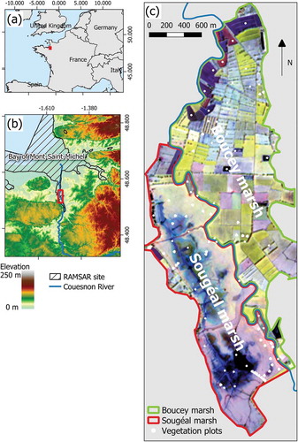
The study site comprises fresh marshes (6–7 m asl) in the Bay of Mont-Saint-Michel (France), which is a RAMSAR and Natura 2000 conservation area (Figure 1). The Couesnon River divides the Sougéal marsh on the west side from the Boucey marsh on the east side. Agricultural and hydraulic management practices differ for each marsh: the Sougéal marsh consists of grazed grasslands, and floodwater is retained to provide a suitable habitat for waterfowl nesting and pike reproduction, while the Boucey marsh consists of mainly of mowed grasslands with efficient water drainage. The landscape consists mainly of grasslands ranging from mesophilic hay Arrhenatherum elatius plant species at the highest elevations to long-flooded Eleocharis palustris and Glyceria fluitans plant species in depressions (Rapinel et al., 2019). A bocage network of alder and willow is present in the Boucey marsh, while poplar plantations exist along the Couesnon River. Crops occur north of the Boucey marsh along the alluvial bank of the Couesnon. Floating aquatic vegetation (Callitriche palustris and Lemna minor) spread over the stagnant water of the Sougéal marsh. A full description of the vegetation classes is provided in Table 1.

Table 1. The vegetation classes studied and respective sample sizes (pixel dimension: 1.5 × 1.5 m)

Class no.	Class name	Sample size (no. of pixels)
1	Arrhenatherum elatius grasslands	6
2	Anthoxanthum odoratum – Bromus racemosus grasslands	15
3	Holcus lanatus – Lolium perenne grasslands	21
4	Trifolium repens – Cirsium arvense grasslands	36
5	Alopecurus geniculatus – Oenanthe fistulosa grasslands	24
6	Eleocharis palustris – Glyceria fluitans grasslands	12
7	Veronica scutellata – Glyceria fluitans grasslands	9
8	Crops (maize, wheat)	9
9	Floating vegetation (Callitriche palustris – Lemna minor)	11
10	Open water	9
11	Woods (Alnus sp., Salix alba, Populus sp.)	18

Figure 1. Location of the study site (a and b) and vegetation plots (c). The color composite is produced from the SPOT-7 pan-sharpened band 4 (blue: 21 April 2017, green: 9 May 2017, red: 17 June 2017)

Field data

Phytosociological surveys in 2 × 2 m quadrats were collected on grasslands in 2017 according to the Braun-Blanquet method (Braun-Blanquet, 1932). Vegetation plots were separated by at least 10 m to minimize spatial autocorrelation. Additional field surveys were conducted to identify dominant plant species and to characterize non-grassland vegetation. In total, 170 vegetation plots were sampled for the 11 vegetation classes studied and were georeferenced using differential GPS (horizontal accuracy < 50 cm).

Satellite images

Four cloud-free and ortho-corrected SPOT-7 images acquired from spring to summer 2017 (April 21, May 9, June 17 and July 7) were provided by the French Space Agency (CNES) in Top of Atmosphere reflectance. SPOT-7 images include one panchromatic band (0.455–0.745 µm) at 1.5 m spatial resolution and four multispectral bands at 6.0 m spatial resolution in the blue (0.455–0.525 µm), green (0.530–0.590 µm), red (0.625–0.695 µm) and near-infrared (0.760–0.890 µm) wavelengths.

A Bayesian fusion of the panchromatic and multispectral bands was performed for each image using the orfeo-toolbox (Grizonnet et al., 2017), resulting in four pan-sharpened bands at 1.5 m spatial resolution. Equations of the baysesian data fusion are detailed in Fasbender et al. (2008). Specifically, the weight parameter – that sets the importance assigned to the panchromatic band with respect to the multispectral image in the fusion process – was used with a default value of 0.9 to enhance the spatial resolution quality of the pan-sharpened bands. Indeed, a low value (close to 0) of the weight parameter assigns high importance to the multispectral image (i.e. to the spectral resolution) while a high value (close to 1) places great emphasis to the panchromatic band (i.e. to the spatial resolution).

Since the wide range of the spectral band values could have strongly influenced the variable importance measures in the modeling procedure (Strobl et al., 2007), all pan-sharpened bands were standardized (overall mean of 0 and standard deviation of 0.25).

Principal component analysis

A principal component analysis (PCA) was calculated on the 16 (4 bands × 4 dates) SPOT-7 standardized spectral variables for the 170 vegetation plots to represent the typical spectrum of each of the 11 vegetation classes. Then, the spectral separability of these vegetation classes was measured using between-class analysis (BCA) based on the coordinates of the PCA axes (Chessel et al., 2004). The significance of the BCA was assessed against 999 permutation tests.

Random forest modeling

RF modeling (Breiman, 2001) was used to predict the 11 vegetation classes using the four pan-sharpened SPOT-7 images. A complete description of the random forest model functioning is detailed in Belgiu and Drăguţ (2016). Two parameters can be adjusted to fit the random forest model: “Ntree” that determines the number of decision trees to be generated, and “Mtry” that sets the number of variables to be randomly selected for each branch of the trees. Since the RF model is little sensitive to the “Ntree” parameter (Belgiu & Drăguţ, 2016), its default value (500) was kept constant during the model fitting. Conversely, the “Mtry” parameter was tested with all possible values during the fitting process.

The RF model was calibrated and validated from the 170 vegetation plots using a repeated k-fold cross-validation, which is a process well adapted to small samples (Kim, 2009) and provides reliable error estimates (Refaeilzadeh et al., 2009). In particular, the original vegetation plots were randomly divided in three folds (i.e. datasets): for the first iteration, two out of the three folds were used to train the model while the third fold was used to validate it. Subsequently, two other iterations were applied such that at each of them another fold was held out for validation while the two remaining ones were intended for training. This 3-fold cross-validation process was repeated 10 times to get a more robust estimation of RF model performance (Kuhn & Johnson, 2013).

The cumulative importance of each spectral band and date was measured by summing the Gini index values (Breiman, 2001) of all bands of the same date or wavelength. Then, the effect of the number of SPOT-7 images used on the RF model’s accuracy was estimated using backward selection. In details, the 4 SPOT-7 images were first ranked according to their cumulative importance (based on the Gini index). Then, the least important image was discarded and the model was cross-validated with the remaining images 3 times until one image. Thus, the 1 date combination holds the best image, the 2 dates combination holds the two best images, etc …

The statistical accuracy of the RF model was provided by the mean and the standard deviation of the overall and class-specific F1 score according to the number of SPOT-7 acquisitions considered. In addition, a cross-validated confusion matrix representing the cumulative distribution error per vegetation class was calculated over the 10 repeats.

The RF model produced two maps: (i) the crisp map, which shows the vegetation class with the highest membership probability for each pixel, and (ii) the uncertainty map, which stores the highest membership probability for each pixel.

RF modeling was performed with R software (R. Core Team, 2019) using the Raster (Hijmans, 2015), randomforest (Breiman et al., 2011) and Caret (Kuhn, 2008) packages.

Results

Spectral ordination

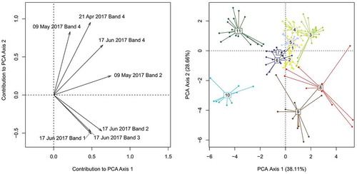
The ordination of vegetation plots on the first two axes of the PCA (66.7% of the total spectral variance) underlines that crops (8), floating vegetation (9), open water (10) and woods (11) classes are clearly distinctive, whereas the grassland vegetation classes (1–7) are separate but slightly mixed together (Figure 2, right), e.g., Eleocharis palustris – Glyceria fluitans grasslands (class 6) and Veronica scutellata – Glyceria fluitans grasslands (class 7), or Arrhenatherum elatius grasslands (class 1) and Anthoxanthum odoratum – Bromus racemosus grasslands (class 2). Moreover, the BCA indicates that the SPOT-7 data differentiate between the 11 vegetation classes since they explain a substantial portion of the spectral variance (76.5%, p-value < 0.001).

Figure 2. (left) Contribution of SPOT-7 variables to the 2 first PCA axes. For clarity, only the most contributing variables (cos2 > 0.7) are shown; (right) PCA ordination diagram outlining the distribution of the vegetation plots according to their membership class (as described in Table 1)

Model accuracy

Accuracy of the RF model of the 11 vegetation classes based on the four SPOT-7 images was high (F1 score 0.88). The confusion matrix (Table 2) indicated that Anthoxanthum odoratum – Bromus racemosus grasslands (class 2), crops (class 8), floating vegetation (class 9), open water (class 10) and woods were modeled accurately (F1 score > 0.9). Arrhenatherum elatius grasslands (class 1), Holcus lanatus – Lolium perenne grasslands (class 3), Trifolium repens – Cirsium arvense grasslands (class 4) and Alopecurus geniculatus – Oenanthe fistulosa grasslands (class 5) were modeled well (F1 score > 0.8). Conversely, the modeling was less accurate for Eleocharis palustris – Glyceria fluitans grasslands (class 6) and Veronica scutellata – Glyceria fluitans grasslands (class 7) (F1 score 0.65–0.77). The largest errors occurred for grassland classes with similar floristic composition: for example, 11% of Holcus lanatus – Lolium perenne grasslands (class 3) were misclassified as Trifolium repens – Cirsium arvense grasslands (class 4); 26% of Eleocharis palustris – Glyceria fluitans grasslands (class 6) were incorrectly classified as Veronica scutellata – Glyceria fluitans grasslands (class 7); and, 22% of class 7 were incorrectly classified as class 6.

Table 2. Cross-validated (3-fold repeated 10 times) confusion matrix between random forest classification of the four SPOT-7 images (rows) and vegetation plots (columns). Entries are cumulative percentage cell counts per column (i.e., number of reference samples per class) over the 10 repeats

		Reference
	Class	1	2	3	4	5	6	7	8	9	10	11
Prediction	1	81.7		0.5
	2	1.7	91.3	9.0
	3			79.0	5.8
	4	3.3	8.7	11.0	88.6	5.0
	5	13.3		0.5	5.6	95.0		13.3		0.9
	6						74.2	22.2			4.4	3.3
	7						25.8	64.4				0.6
	8								98.9
	9								1.1	99.1
	10										90.0	1.1
	11										5.6	95.0
Plot count		60	150	210	360	240	120	90	90	110	90	180
F1 score		0.89	0.90	0.84	0.88	0.89	0.77	0.66	0.99	0.98	0.94	0.96

Cumulative importance scores derived from the Gini index differed greatly among spectral bands and, to a lesser extent, acquisition dates (Figure 3). In particular, the near-infrared spectral band 4 was clearly the most discriminating (cumulative importance of 191), followed by the green band 2 (cumulative importance of 79), blue band 1 and red band 3 (cumulative importance of 31 and 16, respectively). Among acquisition dates, 21 April and 9 May had the most discriminating images (cumulative importance of 108 and 92, respectively), followed by 7 July and 17 June (cumulative importance of 63 and 54, respectively).

Figure 3. Cumulative importance of (a) SPOT-7 acquisition dates and (b) spectral bands for discriminating wetland vegetation based on the random forest model

The modeling accuracy of each vegetation class depended on the number of SPOT-7 dates used (Figure 4). The optimal value of the “Mtry” parameter was set to 3 for 4 images, 4 for 3 images, 1 for 2 images and 2 for 1 image. Overall modeling accuracy (F1 score) ranged from 0.64 (± 0.02) for one date to 0.88 (± 0.01) for four dates. Class-specific results revealed that the minimum number of dates required to achieve satisfactory modeling accuracy (F1 score > 0.8) varied by vegetation class:

• one SPOT-7 date was sufficient for Trifolium repens – Cirsium arvense grasslands (class 4, F1 score 0.82, ± 0.01), crops (class 8, F1 score 0.96, ± 0.01) and woods (class 11, F1 score 0.87, ± 0.01)

• two SPOT-7 dates were required for Holcus lanatus – Lolium perenne grasslands (class 3, F1 score 0.83, ± 0.01)

• three SPOT-7 dates were required for Anthoxanthum odoratum – Bromus racemosus grasslands (class 2, F1 score 0.83, ± 0.01), Alopecurus geniculatus – Oenanthe fistulosa grasslands (class 5, F1 score 0.91, ± 0.01), Eleocharis palustris – Glyceria fluitans grasslands (class 6, F1 score 0.81, ± 0.02), floating vegetation (class 9, F1 score 0.97, ± 0.01) and open water (class 10, F1 score 0.89, ± 0.03)

• four SPOT-7 dates were required for Arrhenatherum elatius grasslands (class 1, F1 score 0.89, ± 0.03) but remained insufficient to model Veronica scutellata – Glyceria fluitans grasslands (class 7, F1 score 0.65, ± 0.03) satisfactorily.

Figure 4. Mean (black line) and standard deviation (grey area) accuracy of the random forest model over the 10 repeats (overall and per vegetation class) expressed as the F1 score as a function of the number of SPOT-7 dates used. The combination of images was based on backward selection from the least to the most important date (see Figure 3): 3 dates (7 July 2017, 09 May 2017 and 21 April 2017), 2 dates (09 May 2017 and 21 April 2017), 1 date (21 April 2017)

Also, addition of the fourth SPOT-7 date (June 17) decreased the modeling accuracy of grassland classes 5 (−0.01), 6 (−0.01) and 7 (−0.07) as well as crops (−0.01) slightly.

Vegetation map

RF modeling generated a crisp vegetation map using the four SPOT-7 images (Figure 5). Overall, differences between the landscapes of the Sougéal and Boucey marshes were obvious: most hygrophilic (classes 4–7) and mesophilic (class 3) grasslands were distributed in the Sougéal marsh, while the mesophilic hay meadows (classes 1–2) covered much of the Boucey marsh. Crops planted in the northern end of the Boucey marsh were also identified well. The fine-grained pattern of the vegetation was mapped adequately: for example, identification of each tree crown revealed the continuity of the bocage network in the Boucey marsh (Figure 5(a)); the floating vegetation detected in ditches of the Sougéal marsh was also captured accurately (Figure 5(b)); and the fine-grained pattern of the grasslands, with vegetation patches of a few pixels, adequately reflected the subtle micro-topographic variations (Figure 5(c)).

Figure 5. Random-forest-based crisp map (left panel) and uncertainty map (right panel). Inset maps focus on a (a) hedged area and (b and c) open marshes with a moisture gradient

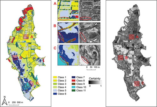
The uncertainty map (Figure 5) indicated that crops (class 8), open water (class 10), floating vegetation (class 9), woods (class 11) and Holcus lanatus – Lolium perenne grasslands (class 3) were mapped with certainty. Conversely, uncertain areas reflected floristic transition zones between two grassland classes (Figure 5(c)) and classes not included in the model (e.g., shadows, mud). For example, tree shadows were classified as long-flooded grassland (class 7) (Figure 5(a)), and ditch-side mud was classified as mesophilic grassland (class 1) (Figure 5(b)).

Discussion

The number of dates required to achieve accurate classification

The use of four pan-sharpened SPOT-7 images modeled 11 vegetation classes accurately (F1 score 0.88). In comparison, previous use of a Sentinel-2 time-series achieved slightly higher modeling accuracy for grassland plant communities (Rapinel et al., 2019), perhaps due to its higher temporal (12 versus 4 acquisition dates) and spectral (10 versus 4 bands) resolution. Moreover, using a single SPOT-7 date decreased modeling accuracy significantly (overall F1 score 0.70), especially for grassland plant communities (F1 score < 0.5 for classes 1, 2, 5 & 6), which is consistent with previous studies based on analysis of one multispectral image (Kumar & Sinha, 2014; Rapinel et al., 2018). The use of three SPOT-7 images is required to achieve high modeling accuracy (overall F1 score > 0.8). In comparison, previous studies applied to wet grassland classes indicated that similar modeling accuracy can be achieved using three optical RapidEye images (T. Schmidt et al., 2014) or five TerraSAR-X images (Betbeder et al., 2015).

However, it should be noted that while the addition of the fourth SPOT-7 image slightly increases the overall accuracy of the RF model, it also slightly reduces the accuracy of 4 vegetation classes. We assume that this is due to the model fitting process that was designed to achieve the highest overall accuracy and not the highest accuracy for specific classes, especially since the sampling between classes was unbalanced (Maxwell et al., 2018). Moreover, the fourth image (June 17) used in this study, which was the least important variable used in the RF model, introduced some noise in the modeling process.

In this study, the estimation of the effect of the number of SPOT-7 images on the RF model accuracy was based on backward selection (i.e. from the least to the most important date) depending on the cumulative Gini index ranking. Although images were standardized to determine the variables of importance (Strobl et al., 2007), it should be kept in mind that the value of the Gini index of each spectral band depends not only on the model fitting method used (here repeated k-fold cross validation) but also on the sample dataset (Kuhn & Johnson, 2013). In other words, the acquisition date ranking and therefore the effect of the number of SPOT-7 images on the RF model accuracy may vary using another model fitting method (e.g. leave-one-out cross-validation) and/or different vegetation plots.

Although reference data may be derived from visual interpretation of images acquired in different years (Gómez et al., 2016), the reference data used in this study were collected by ecologists in the field during spring 2017 according to the phytosociological protocol (Braun-Blanquet, 1932). The advantage of this field-oriented sampling is the quality of the vegetation plots (floristic characterization, georeferencing, no temporal shift with the acquisition of SPOT-7 images). However, collecting field vegetation samples is obviously time-consuming, which results in few, closely spaced vegetation plots. In this context, we minimized model overfitting by separating vegetation surveys by at least 10 m (i.e. six times the SPOT-7 pixel size) (Figure 1). Finally, the consistency of the vegetation map with the ground truth supported the statistical results. Prior visual inspection of the fine-grained pattern of vegetation from UAV images could provide a useful tool to improve sample collection (Nowak et al., 2019).

Although widely used, the k-fold cross-validation process is criticized for the overlapping between training and validation samples across iterations, a fortiori when using a low number of folds (Wong, 2015). Ideally, the model fitting and validation should be based on a 10-fold cross-validation (Refaeilzadeh et al., 2009) using independent validation samples, which is in practice difficult to implement for plant species modeling given the rarity of vegetation plots (Miller, 2010). In this study, the number of folds was limited to 3 and no independent validation samples were used due to the small sample size (170 plots for 11 vegetation classes). However, the cross-validation process was repeated 10 times to provide a reasonable estimate of modeling accuracy (Kuhn & Johnson, 2013), the low standard deviation values of the F1 score achieved in this study (Figure 4) stressing the well-fitting of the RF model. Nevertheless, this issue emphasizes the need to support and use vegetation- plot databases such as the European Vegetation Archive (Chytrý et al., 2016) or the Copernicus In Situ component (Marconcini et al., 2020) to better fit and validate species distribution models based on remotely sensed data.

Spectral bands and dates that contributed the most

Spectral band 4, the near-infrared spectrum, discriminated the 11 vegetation classes the most. Since this spectral band is highly sensitive not only to water (low reflectance) but to photosynthetic activity (high reflectance), it logically discriminates between vegetation classes characterized by flood duration and those characterized by phenological shift (Rapinel et al., 2019). However, unlike the SPOT-5 sensor, the SPOT-6/7 sensors have no middle-infrared band, which is a highly discriminating band for wet vegetation (Davranche et al., 2010).

In the present study, the SPOT-7 images acquired in the spring were clearly the most useful for discriminating the 11 vegetation classes. During this season, the hydrological conditions of the Couesnon marshes vary greatly (Betbeder et al., 2015), which structures the spatial pattern and phenology of each class of grassland vegetation. Defining an optimal date for discriminating wet vegetation is challenging since the latter differs depending on specific environmental conditions, management characteristics and climatic variations. Nevertheless, spring and early summer emerge as the most discriminating periods in temperate climates (Raab et al., 2018; Rapinel et al., 2019; T. Schmidt et al., 2014).

Suitability of the spatial resolution of SPOT-7 images for mapping wetland vegetation

Although the pan-sharpening processing of SPOT-7 images decreased their radiometric resolution, their very high spatial resolution (1.5 × 1.5 m) revealed small patches of vegetation (e.g. grassland plant communities, floating vegetation, tree crowns). At ~1:5,000 scale, the vegetation map derived from SPOT-7 images has a spatial scale similar to that of most field vegetation maps (Pedrotti, 2013). However, the resolution of SPOT-6 images (1.5 × 1.5 m) remains too coarse to detect certain micro-patches of vegetation (< 1 m wide) that can indicate the conservation status of habitats, such as Juncus gerardii salt grassland plant communities (Bouzillé et al., 2001) or invasive species (Evans & Arvela, 2011). Addressing these limitations requires images with a spatial resolution < 0.5 m, such as Worldview images (Collin et al., 2018) or UAV data (Nowak et al., 2019).

Beyond the detailed map scale, the very high spatial resolution of SPOT-7 images is also relevant for sampling vegetation plots, since the pixel size (1.5 × 1.5 m) is similar to the size of phytosociological plots (2 × 2 m) (Braun-Blanquet, 1932). In other words, the field vegetation plots sampled using the Braun-Blanquet protocol can be related easily to a pure pixel, which is not the case when using images with coarse pixels, in which vegetation plots must be collected with a remote-sensing-specific protocol (Rapinel et al., 2019).

Generating an uncertainty map with the traditional crisp vegetation map provides useful information for implementing additional “preferential” sampling (De Cáceres et al., 2015). As expected, broad vegetation classes (e.g. crops, woods) were modeled with certainty given their specific spectral signatures, while grassland community classes were generally modeled with more uncertainty given their spectral similarities (Rocchini et al., 2013). Moreover, providing a complete nomenclature of the studied site is always challenging, especially for large areas. In this context, the uncertainty map is useful since it reveals classes that were not considered in the modeling process due to their sporadic presence, such as shadows, mud or reed beds.

Conclusion

This study highlights the value of multi-temporal SPOT-7 imagery for mapping fine-grained patterns of 11 vegetation classes in wetlands. Specifically, the near-infrared spectral bands acquired in the spring are the most discriminating features. SPOT-7 images have the advantage of combining very high spatial resolution (1.5 × 1.5 m) with a wide swath (60 km), which can be used to model the fine-grained pattern of wetland vegetation over large areas. The uncertainty map, which highlights areas of floristic transition and classes not considered in the modeling process, helps managers and botanists interpret the results and identify additional areas to be prospected in the field. Futures researches will investigate the impact of the spatial resolution of remote sensing data on the detection of plant communities.

Acknowledgments

This study was supported by the French Ministry of Ecology under Grant no. 2101606295. The SPOT-7 data were pre-processed and provided by the CNES (Kalideos program). The field campaigns were supported by the CNRS (Zone Atelier program). The authors are grateful to Cendrine Mony, Lucie Lecoq, and Bernard and Mireille Clément for collecting the phytosociological surveys and for their valuable expertise.

Disclosure statement

The authors report no potential conflict of interest.

Additional information

Funding

This work was supported by the French Ministry of Ecology [2101606295].

References

- Belgiu, M. , & Drăguţ, L. (2016). Random forest in remote sensing: A review of applications and future directions. ISPRS Journal of Photogrammetry and Remote Sensing , 114, 24–31. https://doi.org/10.1016/j.isprsjprs.2016.01.011
- Betbeder, J. , Rapinel, S. , Corgne, S. , Pottier, E. , & Hubert-Moy, L. (2015). TerraSAR-X dual-pol time-series for mapping of wetland vegetation. ISPRS Journal of Photogrammetry and Remote Sensing , 107, 90–98. https://doi.org/10.1016/j.isprsjprs.2015.05.001
- Bijlsma, R. J. , Agrillo, E. , Attorre, F. , Boitani, L. , Brunner, A. , Evans, P. , Foppen, R. , Gubbay, S. , Janssen, J. A. M. , & van Kleunen, A. (2019). Defining and applying the concept of favourable reference values for species habitats under the EU birds and habitats directives : Examples of setting favourable reference values . Wageningen Environmental Research.
- Bouzillé, J.-B. , Kernéis, E. , Bonis, A. , & Touzard, B. (2001). Vegetation and ecological gradients in abandoned salt pans in western France. Journal of Vegetation Science , 12(2), 269–278. https://doi.org/10.2307/3236611
- Braun-Blanquet, J. (1932). Plant sociology. The study of plant communities (1st ed.). McGraw-Hill Book Co., Inc., New York and London.
- Breiman, L. (2001). Random Forests. Machine Learning , 45(1), 5–32. https://doi.org/10.1023/A:1010933404324
- Breiman, L. , Cutler, A. , Liaw, A. , & Wiener, M. (2011). Package randomForest . http://stat-www.berkeley.edu/users/breiman/RandomForests
- Chessel, D. , Dufour, A. B. , & Thioulouse, J. (2004). The ade4 package-I-One-table methods. R News , 4(1), 5–10. http://thioulouse.fr/ref/ade4-Rnews.pdf
- Chytrý, M. , Hennekens, S. M. , Jiménez-Alfaro, B. , Knollová, I. , Dengler, J. , Jansen, F. , Landucci, F. , Schaminée, J. H. , Aćić, S. , & Agrillo, E. (2016). European Vegetation Archive (EVA) : An integrated database of European vegetation plots. Applied Vegetation Science , 19(1), 173–180. https://doi.org/10.1111/avsc.12191
- Collin, A. , Lambert, N. , & Etienne, S. (2018). Satellite-based salt marsh elevation, vegetation height, and species composition mapping using the superspectral WorldView-3 imagery. International Journal of Remote Sensing , 39(17), 5619–5637. https://www.tandfonline.com/doi/abs/10.1080/01431161.2018.1466084
- Davranche, A. , Lefebvre, G. , & Poulin, B. (2010). Wetland monitoring using classification trees and SPOT-5 seasonal time series. Remote Sensing of Environment , 114(3), 552–562. https://doi.org/10.1016/j.rse.2009.10.009
- De Cáceres, M. , Chytrý, M. , Agrillo, E. , Attorre, F. , Botta-Dukát, Z. , Capelo, J. , Czúcz, B. , Dengler, J. , Ewald, J. , Faber-Langendoen, D. , Feoli, E. , Franklin, S. B. , Gavilán, R. , Gillet, F. , Jansen, F. , Jiménez-Alfaro, B. , Krestov, P. , Landucci, F. , Lengyel, A. , & Scheiner, S. (2015). A comparative framework for broad-scale plot-based vegetation classification. Applied Vegetation Science , 18(4), 543–560. https://doi.org/10.1111/avsc.12179
- Evans, D. , & Arvela, M. (2011). Assessment and reporting under article 17 of the habitats directive. Explanatory notes & guidelines for the period 2007-2012 . European Commission.
- Fasbender, D. , Radoux, J. , & Bogaert, P. (2008). Bayesian data fusion for adaptable image pansharpening. IEEE Transactions on Geoscience and Remote Sensing , 46(6), 1847–1857. https://doi.org/10.1109/TGRS.2008.917131
- Gómez, C. , White, J. C. , & Wulder, M. A. (2016). Optical remotely sensed time series data for land cover classification : A review. ISPRS Journal of Photogrammetry and Remote Sensing , 116, 55–72. https://doi.org/10.1016/j.isprsjprs.2016.03.008
- Grizonnet, M. , Michel, J. , Poughon, V. , Inglada, J. , Savinaud, M. , & Cresson, R. (2017). Orfeo ToolBox : Open source processing of remote sensing images. Open Geospatial Data, Software and Standards , 2(1), 15. https://doi.org/10.1186/s40965-017-0031-6
- Hijmans, R. J. (2015). raster : geographic data analysis and modeling . http://CRAN.R-project.org/package=raster
- Kattenborn, T. , Eichel, J. , & Fassnacht, F. E. (2019). Convolutional Neural Networks enable efficient, accurate and fine-grained segmentation of plant species and communities from high-resolution UAV imagery. Scientific Reports , 9(1), 1–9. https://doi.org/10.1038/s41598-019-53797-9
- Kim, J.-H. (2009). Estimating classification error rate: Repeated cross-validation, repeated hold-out and bootstrap. Computational Statistics & Data Analysis , 53(11), 3735–3745. https://doi.org/10.1016/j.csda.2009.04.009
- Kuhn, M. (2008). Caret package. Journal of Statistical Software , 28(5), 1–26. https://doi.org/10.18637/jss.v028.i07
- Kuhn, M. , & Johnson, K. (2013). Applied predictive modeling . Springer-Verlag.
- Kumar, L. , & Sinha, P. (2014). Mapping salt-marsh land-cover vegetation using high-spatial and hyperspectral satellite data to assist wetland inventory. GIScience & Remote Sensing , 51(5), 483–497. https://doi.org/10.1080/15481603.2014.947838
- Mahdavi, S. , Salehi, B. , Granger, J. , Amani, M. , Brisco, B. , & Huang, W. (2018). Remote sensing for wetland classification : A comprehensive review. GIScience & Remote Sensing , 55(5): 623-658. https://doi.org/10.1080/15481603.2017.1419602
- Mahdianpari, M. , Salehi, B. , Mohammadimanesh, F. , Brisco, B. , Mahdavi, S. , Amani, M. , & Granger, J. E. (2018). Fisher linear discriminant analysis of coherency matrix for wetland classification using PolSAR imagery. Remote Sensing of Environment , 206, 300–317. https://doi.org/10.1016/j.rse.2017.11.005
- Maltby, E. , & Barker, T. (2009). The Wetlands Handbook . Wiley-Blackwell.
- Marcinkowska-Ochtyra, A. , Gryguc, K. , Ochtyra, A. , Kopeć, D. , Jarocińska, A. , & Sławik, Ł. (2019). Multitemporal hyperspectral data fusion with topographic indices—Improving classification of Natura 2000 grassland habitats. Remote Sensing , 11(19), 2264. https://doi.org/10.3390/rs11192264
- Marconcini, M. , Esch, T. , Bachofer, F. , & Metz-Marconcini, A. (2020). Digital earth in Europe. In H. Guo , M.F. Goodchild , & A. Annoni (Eds.), Manual of digital earth (pp. 647–681). Springer. https://doi.org/10.1007/978-981-32-9915-3_20
- Maxwell, A. E. , Warner, T. A. , & Fang, F. (2018). Implementation of machine-learning classification in remote sensing : An applied review. International Journal of Remote Sensing , 39(9), 2784–2817. https://doi.org/10.1080/01431161.2018.1433343
- Miller, J. (2010). Species distribution modeling. Geography Compass , 4(6), 490–509. https://doi.org/10.1111/j.1749-8198.2010.00351.x
- Mohammadimanesh, F. , Salehi, B. , Mahdianpari, M. , Motagh, M. , & Brisco, B. (2018). An efficient feature optimization for wetland mapping by synergistic use of SAR intensity, interferometry, and polarimetry data. International Journal of Applied Earth Observation and Geoinformation , 73, 450–462. https://doi.org/10.1016/j.jag.2018.06.005
- Nowak, M. M. , Dziób, K. , & Bogawski, P. (2019). Unmanned Aerial Vehicles (UAVs) in environmental biology : A review. European Journal of Ecology , 4(2), 56–74. https://doi.org/10.2478/eje-2018-0012
- Paganini, M. , Leidner, A. K. , Geller, G. , Turner, W. , & Wegmann, M. (2016). The role of space agencies in remotely sensed essential biodiversity variables. Remote Sensing in Ecology and Conservation , 2(3), 132–140. https://doi.org/10.1002/rse2.29
- Pedrotti, F. (2013). Plant and vegetation mapping . Springer.
- R. Core Team . (2019). A language and environment for statistical computing. Vienna, Austria : R foundation for statistical computing; 2012 . https://www. R-project. org
- Raab, C. , Stroh, H. G. , Tonn, B. , Meißner, M. , Rohwer, N. , Balkenhol, N. , & Isselstein, J. (2018). Mapping semi-natural grassland communities using multi-temporal RapidEye remote sensing data. International Journal of Remote Sensing , 39(17), 5638–5659. https://doi.org/10.1080/01431161.2018.1504344
- Rapinel, S. , Clément, B. , Magnanon, S. , Sellin, V. , & Hubert-Moy, L. (2014). Identification and mapping of natural vegetation on a coastal site using a Worldview-2 satellite image. Journal of Environmental Management , 144, 236–246. https://doi.org/10.1016/j.jenvman.2014.05.027
- Rapinel, S. , Mony, C. , Lecoq, L. , Clément, B. , Thomas, A. , & Hubert-Moy, L. (2019). Evaluation of Sentinel-2 time-series for mapping floodplain grassland plant communities. Remote Sensing of Environment , 223, 115–129. https://doi.org/10.1016/j.rse.2019.01.018
- Rapinel, S. , Rossignol, N. , Hubert-Moy, L. , Bouzillé, J.-B. , & Bonis, A. (2018). Mapping grassland plant communities using a fuzzy approach to address floristic and spectral uncertainty. Applied Vegetation Science , 21(4), 678–693. https://doi.org/10.1111/avsc.12396
- Refaeilzadeh, P. , Tang, L. , & Liu, H. (2009). Cross-validation. In Encyclopedia of database systems (pp. 532–538). New York: Springer.
- Rocchini, D. , Foody, G. M. , Nagendra, H. , Ricotta, C. , Anand, M. , He, K. S. , Amici, V. , Kleinschmit, B. , Förster, M. , Schmidtlein, S. , Feilhauer, H. , Ghisla, A. , Metz, M. , & Neteler, M. (2013). Uncertainty in ecosystem mapping by remote sensing. Computers & Geosciences , 50, 128–135. https://doi.org/10.1016/j.cageo.2012.05.022
- Schmidt, J. , Fassnacht, F. E. , Lausch, A. , & Schmidtlein, S. (2017). Assessing the functional signature of heathland landscapes via hyperspectral remote sensing. Ecological Indicators , 73, 505–512. https://doi.org/10.1016/j.ecolind.2016.10.017
- Schmidt, T. , Schuster, C. , Kleinschmit, B. , & Förster, M. (2014). Evaluating an intra-annual time series for grassland classification #x2014;How many acquisitions and what seasonal origin are optimal? IEEE Journal of Selected Topics in Applied Earth Observations and Remote Sensing , 7(8), 3428–3439. https://doi.org/10.1109/JSTARS.2014.2347203
- Schuster, C. , Schmidt, T. , Conrad, C. , Kleinschmit, B. , & Förster, M. (2015). Grassland habitat mapping by intra-annual time series analysis – Comparison of RapidEye and TerraSAR-X satellite data. International Journal of Applied Earth Observation and Geoinformation , 34, 25–34. https://doi.org/10.1016/j.jag.2014.06.004
- Silva, V. , Catry, F. X. , Fernandes, P. M. , Rego, F. C. , Paes, P. , Nunes, L. , Caperta, A. D. , Sérgio, C. , & Bugalho, M. N. (2019). Effects of grazing on plant composition, conservation status and ecosystem services of Natura 2000 shrub-grassland habitat types. Biodiversity and Conservation , 28(5): 1205-1224. https://doi.org/10.1007/s10531-019-01718-7
- Stehman, S. V. , & Foody, G. M. (2019). Key issues in rigorous accuracy assessment of land cover products. Remote Sensing of Environment , 231, 111199. https://doi.org/10.1016/j.rse.2019.05.018
- Strobl, C. , Boulesteix, A.-L. , Zeileis, A. , & Hothorn, T. (2007). Bias in random forest variable importance measures : Illustrations, sources and a solution. BMC Bioinformatics , 8(1), 25. https://doi.org/10.1186/1471-2105-8-25
- Ullerud, H. A. , Bryn, A. , Halvorsen, R. , & Hemsing, L. Ø. (2018). Consistency in land cover mapping : Influence of field workers, spatial scale and classification system. Applied Vegetation Science , 21(2), 278–288. https://doi.org/10.1111/avsc.12368
- Van Beijma, S. , Comber, A. , & Lamb, A. (2014). Random forest classification of salt marsh vegetation habitats using quad-polarimetric airborne SAR, elevation and optical RS data. Remote Sensing of Environment , 149, 118–129. https://doi.org/10.1016/j.rse.2014.04.010
- Wang, R. , & Gamon, J. A. (2019). Remote sensing of terrestrial plant biodiversity. Remote Sensing of Environment , 231, 111218. https://doi.org/10.1016/j.rse.2019.111218
- Wong, -T.-T. (2015). Performance evaluation of classification algorithms by k-fold and leave-one-out cross validation. Pattern Recognition , 48(9), 2839–2846. https://doi.org/10.1016/j.patcog.2015.03.009
- Yao, H. , Qin, R. , & Chen, X. (2019). Unmanned aerial vehicle for remote sensing applications—A review. Remote Sensing , 11(12), 1443. https://doi.org/10.3390/rs11121443
- Zlinszky, A. , Schroiff, A. , Kania, A. , Deák, B. , Mücke, W. , Vári, Á. , Székely, B. , & Pfeifer, N. (2014). Categorizing Grassland vegetation with full-waveform airborne laser scanning : A feasibility study for detecting Natura 2000 habitat types. Remote Sensing , 6(9), 8056–8087. https://doi.org/10.3390/rs6098056