Fluvial gravel bar mapping with spectral signal mixture analysis

1

ABSTRACT

The paper presents a method for mapping fluvial gravel bars based on Sentinel-2 and Landsat imagery. The proposed method therefore uses spectral signal mixture analysis (SSMA) because its results allow the development of land cover fraction maps for surface water, gravel, and vegetation. The method is validated on a spatially heterogeneous mountainous area in the upper Soča river basin in north-west Slovenia, Central Europe. Unmixing results in highly accurate fraction maps with MAE of around 0.1. Gravel fractions are mapped the most accurately, indicating that the approach can be used successfully for fluvial gravel bar mapping. Endmember sets selected automatically perform slightly worse (MAE higher by at most 0.05) than sets selected manually based on high resolution reference data. Both Sentinel-2 and Landsat imagery can be used for accurate mapping with differences between the two remote sensing systems within 0.05 MAE. For the study area, the SSMA-based soft classification method is more accurate for land cover mapping than a Spectral Angle Mapping-based hard classification. The method is promising for an effective use in other cases where highly accurate subpixel information is needed, because it is able to detect small-scale changes that could go unnoticed with hard classification mapping.

KEYWORDS:

• Geomorphology
• rivers
• sub-pixel
• alpine
• multispectral data
• mapping

Introduction

Fluvial gravel bars are important habitats for different species of birds (Denac & Božič, 2012; Zeng et al., 2015), invertebrates (Langhans & Tockner, 2014), and plants (Geršič, 2010). In addition to the importance for biodiversity, gravel bars play a role in water filtration, groundwater infiltration, mitigation of river bank erosion, and in increasing the river’s attractiveness for recreation (Robert, 2003). Anthropogenic factors such as dam construction and other flood control infrastructure, as well as natural factors such as increased rainfall and consequently a larger runoff, have an impact on the location and extent of gravel bars (Assani & Petit, 2004). Their existence is threatened by gravel harvesting for industrial use (Jogan et al., 2004). Gravel bars are sensitive to hydrological changes and are therefore considered to be reliable indicators of disturbances in the fluvial and riparian environments (Kiss & Andrási, 2017).

Extent and location monitoring of fluvial gravel bars is usually done using manual delineation based on aerial orthophotos (Geodetic Institute of Slovenia, 2017) or satellite imagery (Serlet, 2018). Characteristics such as good spatial, radiometric, and spectral resolution, multi-level monitoring capability (local, regional, global), frequent revisit times, and free and open accessibility have made satellite imagery an established source of environmental data (De Sherbinin et al., 2014).

Several remote sensing products have already been developed to monitor the extent of surface water ecosystems on a global scale (Huang et al., 2018). The most widely used is the Global Surface Water Explorer, developed at the European Commission’s Joint Research Center (Pekel et al., 2016). Similar products monitor the extent of surface water over time (Donchyts et al., 2016), or focus on particular surface water forms, such as lakes (Verpoorter et al., 2014), wetlands (Prigent et al., 2001), and rivers (Allen & Pavelsky, 2018). The main disadvantage of these products is their coarse spatial resolution, which is generally not better than 30 m. This is very good for a global review, but it may lead to incomplete data at more detailed spatial levels. This limitation is particularly pronounced in areas with high spatial fragmentation of land use, which is also characteristic of Slovenia (Foški, 2017; Hladnik, 2005). The upstream sections of rivers in mountainous areas present a typical challenge.

To mitigate constraints related to the spatial resolution of satellite imagery, the proposed method for mapping the land cover of fluvial and riparian ecosystems relies on spectral signal mixture analysis (SSMA) (Atkinson, 2005; Foody et al., 2005). The SSMA determines the proportion of the selected land cover classes present within each pixel based on the pixel’s values in different wavelengths. Thus, a sub-pixel mapping accuracy can be achieved (e.g., Ling et al., 2016; Mylona et al., 2018). The key information for the SSMA is the spectral reflectance of pure pixels (endmembers), i.e. the pixels that contain only one land cover class (Somers et al., 2011; Veganzones & Graña, 2008). These endmembers represent the extreme points in the spectral space (Keshava, 2003).

The main objective of this study is to evaluate the potential of SSMA to monitor the location and extent of fluvial gravel bars. Four objectives were set to achieve this:

1. to examine the accuracy of SSMA for mapping active gravel bars, surface water and riparian vegetation,

2. to study the difference between using manually and automatically selected endmembers for mapping fluvial and riparian land cover fractions,

3. to assess the suitability of different multispectral remote sensing systems for mapping land cover fractions in fluvial and riparian ecosystems, and

4. to evaluate the soft classification method compared to the hard classification method.

Materials and methods

Study area

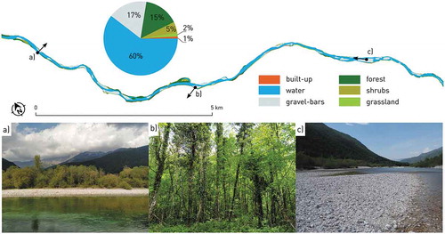
The method was validated on an approximately 15 km long section in the upper Soča river basin in north-western Slovenia, Central Europe, centred on 46.2° north and 13.6° east (Figure 1). The bedrock in the area is composed of limestone and dolomite (Geological Survey of Slovenia, 2019). The climate ranges from mountainous to temperate Mediterranean (Ogrin & Plut, 2009) and the river basin is characterized by a nivo-pluvial flow regime. The main discharge peak occurs in April or May due to snow melt, and the secondary discharge peak usually occurs in November due to autumn rainfall. The low winter discharge that results from temporal storage of precipitation as snow is more pronounced than the low summer discharge, which usually occurs in August due to high evapotranspiration (Ogrin & Plut, 2009). As a result of the intense hydromorphological processes conditioned by terrain topography and hydrological characteristics, Soča transports some of the highest amounts of gravel in Slovenia (Ranfl, 2010). Several fluvial gravel bars form on the selected section, making it well-suited as a validation area. Additionally, Soča is a very narrow water body, particularly in its upper reaches, often not exceeding 20 m in width. The region of interest is therefore ideal for a study of the potentials of using SSMA for gravel bar detection. The specific study area was selected based on the vector layer of water-related parcels (Slovenian Water Agency, 2018b), which comprises surface water bodies up to the first geomorphological change (Geodetic Institute of Slovenia, 2017). Land cover of the study area is comprised mostly of surface water, followed by gravel bars and deciduous forest (Figure 2).

Figure 1. Overview of the study area. a) Location of the study site (red rectangle) in the upper Soča river basin, north-western Slovenia, Central Europe, centred on 46.2° north and 13.6° east (data source: Natural Earth, 2020). b) A closer view of the study area. The red rectangle indicates the whole study area while the purple rectangle marks the location of the zoomed-in view in Figure 8 (data source: Surveying and Mapping Authority of the Republic of Slovenia, 2016). c) – f) True colour composites of images used in the analysis. Remote sensing system and acquisition date indicated in the lower right

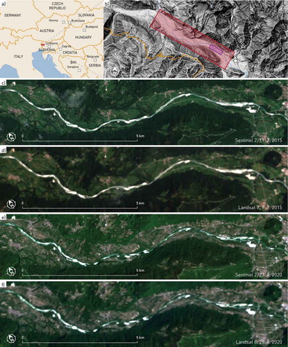
Figure 2. Land cover in the study area. Arrows indicate viewing direction of photographs (data source: Ministry of Agriculture, Forestry and Food of the Republic of Slovenia, 2020; Slovenian Water Agency, 2018a; photographs: Liza Stančič)

Remote sensing data

We performed gravel bar mapping in several successive steps (Figure 3). Following the objectives of the study, we used aerial orthophotos and satellite imagery of very similar dates. We selected orthophotos acquired on 26. 6. 2015 as a reference data source, and the closest satellite images without cloud cover over the study areas. These were a Landsat 7 image acquired on 9. 7. 2015 and a Sentinel-2 image acquired on 11. 7. 2015. We also analysed more recent imagery, namely a Landsat 8 image acquired on 25. 4. 2020 and a Sentinel-2 image acquired on 23. 4. 2020. Results based on the 2020 imagery were validated with field mapping data.

Figure 3. Workflow for spectral signal mixture analysis for subpixel mapping of fluvial gravel bars

Spectral bands 1–5 and 7 of Landsat 7, 1–7 and 9 of Landsat 8, and 1–8A, 11, and 12 of Sentinel-2 were used for the SSMA. Additionally, we calculated several spectral indices for better differentiation between gravel, vegetation, and water (Table 1): Modified Soil Adjusted Vegetation Index (MSAVI2) (Qi et al., 1994), Normalised Difference Infrared Index (NDII) (Gao, 1996), Normalised Difference Vegetation Index (NDVI) (Tucker, 1979), green band multiplied by NDVI (NDVI-GREEN) (Švab Lenarčič, 2018), Normalised Difference Water Index (NDWI) (McFeeters, 1996), and Modified Normalised Difference Water Index (MNDWI) (Du et al., 2016).

Table 1. Spectral indices calculated to augment land cover class separability

name	formula	reference
Modified Soil Adjusted Vegetation Index (MSAVI2)	$MSAVI2=\frac{2SWIR+1-\sqrt{{\left(2SWIR+1\right)}^2-8\left(SWIR-NIR\right)}}{2}$	Qi et al., 1994
Normalised Difference Infrared Index (NDII)	$NDII=\frac{NIR-SWIR}{NIR+SWIR}$	Gao, 1996
Normalised Difference Vegetation Index (NDVI)	$NDVI=\frac{NIR-RED}{NIR+RED}$	Tucker, 1979
green band multiplied by NDVI (NDVI-GREEN)	$NDVIGREEN=GREEN\ast \frac{NIR-RED}{NIR+RED}$	Švab Lenarčič, 2018
Normalised Difference Water Index (NDWI)	$NDWI=\frac{GREEN-NIR}{GREEN+NIR}$	McFeeters, 1996
Modified Normalised Difference Water Index (MNDWI)	$MNDWI=\frac{GREEN-SWIR}{GREEN+SWIR}$	Du et al., 2016

The Landsat and Sentinel-2 imagery is geometrically corrected by the provider (USGS and ESA, respectively). Atmospheric corrections were made using the STORM processing chain (Pehani et al., 2016). The processing chain uses ATCOR software (Richter & Schläpfer, 2019) for atmospheric correction and cloud detection. The study aimed to include all of the Sentinel-2 bands with a 20 m or higher spatial resolution. We resampled the 10 m resolution spectral bands of Sentinel-2 to 20 m, using bilinear interpolation. After the pre-processing, the reflectance in the imagery is due solely to the surface characteristics, making the imagery suitable for further analysis.

Field mapping

To ensure the selection of spectrally pure pixels and to validate the fraction maps, we carried out a field mapping campaign of the study area from 25. 4. 2020 to 3. 5. 2020. We mapped five different land cover classes on 50 randomly selected plots, each one 60 m by 60 m in size, and later aggregated them to the three land cover classes of interest – gravel, vegetation, and surface water. The plot size was determined so that at least one pixel in each of the analysed images would fit fully into each of the mapped plots. We used the most recent orthophotos, taken on 14. 10. 2017 (Surveying and Mapping Authority of the Republic of Slovenia, 2017), as a background for field mapping, which we carried out at a scale of 1: 1,000.

Selection of pure pixels

The next step in the analysis involved selecting pure pixels and retrieving their spectral signatures. The land cover classes of interest were vegetation, surface water, and gravel. Pure pixel or endmember selection was done both manually and automatically. Automatic endmember selection (also known as endmember extraction) was carried out using an implementation of the N-FINDR algorithm (Winter, 1999) in the pysptools Python package (version 0.15.0, Therien, 2018). The algorithm searches for a specified number of endmembers which form the extreme points of a geometric body with the maximum possible volume in the multidimensional spectral space. A random selection of pixels is considered in the beginning and the volume of the geometric body that these pixels define is calculated. Next, one of the pixels is swapped by a different pixel that has not yet been considered and the volume of the geometric body is calculated again. If the newly computed volume is bigger than the previous volume, the first pixel is replaced by the second one as a potential endmember. The process continues until no further pixel replacements can be made (Winter, 1999). We began by selecting three different endmembers, and increased this number until all of the three land covers of interest were represented. Five endmembers were selected on Landsat 7 and both Sentinel-2 images; one for gravel, two for vegetation, and two for water. On the Landsat 8 image, six endmembers were selected – one for gravel, three for vegetation, and two for water. The land cover class represented by the selected endmember was determined by checking the endmember location on an aerial orthophoto.

The manual endmember selection involved choosing pure pixels from satellite imagery, and calculating averages from the reflectance values of individual samples to obtain the typical spectral signatures of the land cover classes of interest. For the imagery acquired in 2015, pixel purity was verified using orthophotos taken 13 and 15 days before the Landsat 7 and Sentinel-2 images, respectively (Surveying and Mapping Authority of the Republic of Slovenia, 2015). For the 2020 imagery, the necessary reference data was acquired with field mapping. To select the same number of samples at the same locations for all imagery, we first selected samples on the Landsat 8 image. Sample selection was most limited on this image due to a large pixel size which leads to many mixed pixels. In total, four pure pixels were selected for gravel, nine for water, and 20 for vegetation (Figure 4). Samples were taken at the same locations for all imagery, provided the land cover did not change. If reference data suggested land cover change, we selected a nearby pure sample. To ensure that good samples with a high spectral separability were selected, we calculated the spectral angles between different samples (Figure 5). Spectral separability is the highest between vegetation and water samples, and lowest between gravel and water samples on all imagery. In spite of efforts to select spectrally pure pixels, the river in the study area is rarely more than 2 m deep so the sensors also detect reflectance from the riverbed, leading to mixed spectral signals.

Figure 4. Number of samples collected on each image per selected land cover class

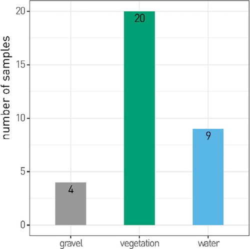
Figure 5. Spectral distances between the manually selected samples of different land cover classes on the analysed satellite images. Values indicate spectral angles in radians

A set of endmembers was selected for each image separately. Assessing the transferability of samples from one image to another was considered outside the scope of this study. Using the methods described above, we obtained a set of endmembers with distinct spectral signatures (Figure 6) and characterised by specific index values (Figure 7). Spectral signatures of automatically and manually selected endmembers have similar overall shapes on all images, however, the reflectance values are different. It is apparent that the automatic method selects pixels with extreme spectral characteristics while the manual method results in a more general spectral signature. For example, in the case of gravel, which is characterised by high reflectance values in all wavelengths, the reflectance values of the automatically selected endmember are higher than those of the manually selected one. Vegetation is modelled with two or three automatically selected endmembers, one for grass (vegetation 1), one for forest (vegetation 2), and in the case of Landsat 8 an additional one for shrubs (vegetation 3). The reflectance values of the manually selected vegetation endmembers are half way between the automatically selected grass and forest endmembers. For water, the reflectance values of the automatically selected endmembers are sometimes higher (as in the case of Landsat 8) and sometime lower (Sentinel-2 2015) than the values of the manually selected endmembers. Spectral signature shapes are similar to those reported in the literature both for Landsat (Afrasinei et al., 2018; Wu, 2004) and for Sentinel-2 (Mylona et al., 2018). The spectral signatures of gravel are very similar to those of built-up land from the literature, while forest (vegetation 2) is less bright than reported in similar studies (Xi et al., 2019), possibly due to terrain shadow.

Figure 6. Spectral signatures of selected endmembers per image and land cover class. A solid line indicates manually selected endmembers while a dashed line indicates endmembers selected automatically

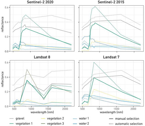
Figure 7. Values of selected indices for the land cover classes considered in the analysis per image. Squares indicated manually selected endmembers while triangles indicate endmembers that were selected automatically. Connecting lines are added for easier detection of values relating to the same land cover class. A solid line indicates manually selected endmembers while a dashed line indicates endmembers selected automatically

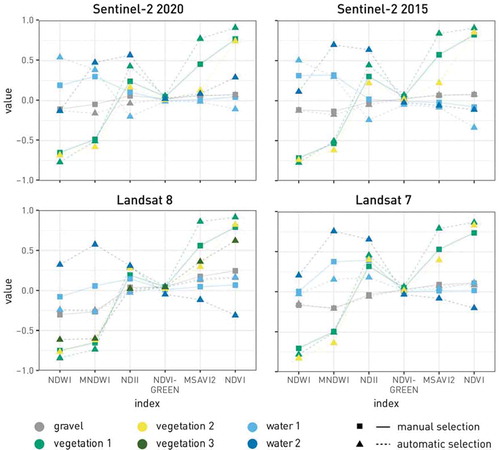
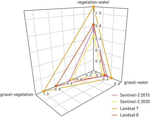
When considering different indices, MNDWI, NDWI, and NDVI values display the highest separability of different land cover classes, followed by MSAVI2. The NDII and NDVI-GREEN index values show a high overlap of different land cover classes. As in the case of reflectance values, it is apparent that the automatically selected endmembers have more extreme index values than the manually selected ones. This is especially true for the vegetation and water endmembers, while for the gravel ones, there is a lot of overlap between the automatically and manually selected endmembers. The index values are in line with those reported in the literature both for manually and for automatically selected endmember (Du et al., 2016; Liu et al., 2020; McFeeters, 1996; Qi et al., 1994; Tucker, 1979). Vegetation endmembers have high index values in MSAVI-2 and NDVI, and low values in NDWI and MNDWI. The opposite is true for water endmembers. The index values of gravel endmembers are mostly in the middle between vegetation and water. An exception is the NDII in which gravel has the lowest value.

Spectral signal mixture analysis (SSMA)

The SSMA was developed to observe rock surface and mineral composition on Mars (Adams et al., 1986). Since then, it has been used for various purposes, including land cover mapping (Ling et al., 2016), determining land cover fractions in urban areas (Kärdi, 2007), soil degradation monitoring (Dubovyk et al., 2015), grassland monitoring (Shao et al., 2018), river bank mapping (Niroumand-Jadidi & Vitti, 2017), and coastline mapping (Foody et al., 2005; Muslim et al., 2007). The SSMA has been used to analyse hyperspectral (Keshava, 2003; Somers et al., 2011) and multispectral satellite imagery, including Landsat (Wu, 2004) and Sentinel-2 (Mylona et al., 2018).

The SSMA works by modelling the reflectances of mixed pixels. In this way, the reflectance in a satellite image is converted to land cover fractions (also known as abundances) of the selected land cover classes based on the spectral characteristics of the endmembers, i.e. spectral representations of pure land cover classes. Modelling methods can be divided into linear and nonlinear. The choice of the model depends on the assumed mechanism of the spectral signal mixing. Linear mixing of reflectance occurs when the considered land cover classes appear in spatially bounded forms. The main physical assumption for linear SSMA is that each input photon reacts with only one land cover type. On the other hand, nonlinear mixing is typical for cases where different types of land cover are closely intertwined. In this case, reflectance mixing is more complex because each input photon reacts with several different land cover types (Keshava, 2003; Keshava & Mustard, 2002).

Given the assumptions, therefore, the mixed pixel signal (r) can be described as a linear combination of endmember spectral signals, weighted by the sub-pixel land cover fraction. The model can be described by (Adams et al., 1986; Somers et al., 2011):

(1) $r=Mf+\epsilon ,$(1)

where M is an array in which each column represents the spectral signature of the selected endmembers, f is the vector of land cover fractions, and ε is the noise or the fraction of a signal that cannot be modelled using the selected endmembers.

The equation can be solved when the endmembers’ spectral signatures are known and the number of endmembers is lower than the number of spectral bands in the analysed image. Quadratic programming, the maximum likelihood method, and the least-squares method are often used to solve the equation. The SSMA can be implemented without restrictions, but to obtain physically meaningful results, it is common to constrain the values of the coefficients in Equation 1(1) $r=Mf+\epsilon ,$(1) to positive numbers. Occasionally, the condition that the sum of the coefficients must be equal to one is also applied, resulting in a so-called fully constrained SSMA (Somers et al., 2011).

Based on the spectral signatures of the land cover classes of interest, a linear SSMA was performed in the selected area using the pysptools Python package (version 0.15.0, Therien, 2018). We applied an implementation of a fully constrained non-negative least squares solver. The SSMA calculates per-pixel fraction of each of the land cover classes of interest. The shares must be positive and must sum to one. Using this information, land cover class fraction maps were produced. Where several different endmembers were selected to represent a single land cover class (i.e. for models based on automatically selected endmembers), their calculated fractions were summed up to obtain the three selected land cover classes of interest.

Evaluation of SSMA for fluvial gravel bar mapping

The suitability of SSMA for fluvial gravel bar mapping was determined in two ways:

1. by analysing the accuracy of the SSMA-derived land cover fraction maps assessed by comparison to reference data, and

2. by comparing the soft and hard classification through an assessment of their respective error metrics, and analysing the accuracy of land cover composition representation.

Accuracy assessment was carried out by comparing the land cover class fractions calculated by SSMA to land cover fractions as determined on reference data using a pixel-wise method (Schug et al., 2018). Orthophotos were used to validate the 2015 imagery while field mapping was used to validate the 2020 imagery. In each case, 50 random plots were selected that were of the same size as the spatial resolution of the satellite imagery and covered exactly one pixel. A regular grid of 100 points was established within each plot, and the land cover class on each point location was determined. The reference fractions were compared to fractions calculated by the SSMA, using the mean average error (MAE).

Results of the soft classification were assessed by comparing them to a hard classification. This was carried out by means of comparing the error metrics of the two different classification methods (Dennison et al., 2004). The commonly used error metric to describe the suitability of SSMA models is RMSE (Dubovyk et al., 2015; Somers et al., 2011). Based on the calculated presence probabilities of the land cover classes of interest, the predicted reflectance values of the input spectral bands are calculated for each individual pixel. The RMSE is then calculated from the average differences between the modelled and the measured reflectance in each of the image bands. We used Spectral Angle Mapper (SAM) (Kruse et al., 1993) for comparison as the hard classification method. Endmembers selected for SSMA were used for classification with SAM on all of the test images. Spectral angle is reported as an error metric of SAM. The spectral angle shows the difference between the reflectance values of a pixel and the reflectance values of the endmember representing the land cover class to which the pixel was assigned. Consequently, the larger the spectral angle of a pixel, the more the pixel’s spectral signature is different to that of the land cover class to which the pixel was classified. For error comparison, 1,000 random pixels were selected on each image and their RMSE values compared against their spectral angles in the pixel-wise majority class. Additionally, the suitability of the SSMA in comparison to SAM for land cover mapping was assessed on a pixel-wise and validation area-wise scale. First, the accuracy of representing the land cover composition on individual pixels was assessed on 50 randomly selected pixels. Next, the accuracy of mapping the land cover on the validation area was evaluated by comparing the land cover presence values per land cover class combined from all of the reference pixels to values obtained by soft and hard classification. We expected that soft classification will performer better than hard classification in the pixel-wise assessment, but we were interested in the influence of increasing the size of the observation unit on the soft and hard classification accuracy.

Results

Land cover fraction maps

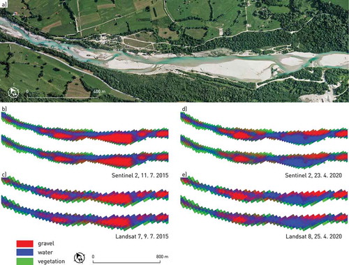
Based on the selected endmembers, we produced land cover fraction maps depicting the presence of gravel, water, and vegetation for the analysed images (Figure 8). Fraction maps appear informative. Location of different land cover classes overlaps well with reference data for the 2015 imagery. For the 2020 imagery, changes in gravel bar size and location can be clearly seen. No major differences can be observed between fraction maps produced with manually or automatically selected endmembers. The biggest discrepancy between different endmember selection methods can be observed on Landsat 7, where models based on manually selected endmembers result in higher gravel fractions and lower water fractions compared to models based on automatically selected endmembers.

Figure 8. Fraction maps for the zoomed-in area, marked by a purple rectangle in Figure 1 b). a) Aerial orthophoto of the area acquired on 26. 6. 2015 (data source: Surveying and Mapping Authority of the Republic of Slovenia, 2015). b) – e) Fraction maps generated with manually selected endmembers shown on top and fraction maps generated with automatically selected endmembers shown on the bottom. Remote sensing system and acquisition date indicated in lower right

The SSMA quality check was performed by examining the MAE values of each analysed image per land cover class and per endmember selection method (Table 2). The lowest error was achieved when classifying the Landsat 8 imagery. Gravel bar fractions were modelled most accurately of all the considered land cover classes on all imagery apart from Sentinel-2 from 2020 where water fractions were determined more correctly. Vegetation fractions were calculated the least accurately, except on Landsat 7 imagery where water fractions had a higher error. In all cases, manually selected endmembers produced more accurate results than endmembers that were selected automatically. Nevertheless, the difference between the manual and automatic endmember selection resulted in MAE differences of at most 0.05.

Table 2. Pixel-wise mean average error per land cover class for different analysed imagery using different endmember selection methods. Acquisition date stated after remote sensing system name. Best results in bold

land cover class	Landsat 7–9. 7. 2015		Sentinel-2 – 11. 7. 2015		Landsat 8–25. 4. 2020		Sentinel-2 – 23. 4. 2020
	manual	automatic	manual	automatic	manual	automatic	manual	automatic
gravel	0.09	0.09	0.08	0.08	0.07	0.07	0.10	0.12
water	0.12	0.14	0.08	0.10	0.07	0.10	0.08	0.10
vegetation	0.11	0.14	0.11	0.14	0.11	0.12	0.11	0.16
sum	0.11	0.12	0.09	0.11	0.08	0.10	0.09	0.13

Comparison of a soft and a hard classification

The results of the soft classification with SSMA were set against the results of a hard classification with SAM using identical endmembers in each case. We assessed the respective error metrics, and compared the results by land cover class, by remote sensing system, and by endmember selection method (Figure 9). For brevity, only the comparison of images acquired in 2020 is shown here. Manual and automatic endmember selection methods were assessed based on the results from the Sentinel-2 imagery. Sentinel-2 and Landsat 8 were compared based on models using automatically selected endmembers. There does not appear to be a strong linear relationship between the two error metrics for any of the models considered. Linear regression of spectral angle against RMSE showed very weak correlations. The highest R² value was calculated for vegetation on the Landsat 8 image; it did not exceed 0.36. This shows that hard classification and soft classification errors are not related. For example, a pixel, that was classified well by the soft classification was not necessarily classified equally well by the hard classification. On the Landsat 8 image, for instance, water pixels generally had a low RMSE but a large spectral angle. For both soft and hard classification, model errors were the lowest and most clustered for gravel, and the highest and most wide-ranging for water. Gravel appears to have a relatively uniform spectral response which can be accurately modelled even based on few samples. Water, on the other hand, has a highly variable spectral response due to the variations in its characteristics, and is thus difficult to represent even with several different samples. In the study area, water depth varies between only a few centimetres to several metres. This leads to the river bed being sometimes included in the spectral signal. Furthermore, rapids are present on some sections of the river resulting in whitewater which has a different spectral response than the less turbulent sections of the river. Manually selected endmembers result in smaller spectral angles but higher RMSE than automatically selected endmembers. This is due to the inherent characteristics of automatically and manually selected endmembers. The automatic method selects endmembers which have the most extreme spectral characteristics and consequently the biggest spectral angle in relation to the spectral responses of other pixels. Conversely, manually selected endmembers represent average spectra which are more similar to a wider range of other spectra, leading to a small spectral angle, but cannot account for the whole range of spectral variability in the image, resulting in a high RMSE. Models for Landsat 8 were comparable to Sentinel-2 for gravel with low RMSE as well as small spectral angles. Gravel appears to be modelled successfully on images from both remote sensing systems. For vegetation, both sensors achieved a comparable RMSE while spectral angles were larger for Landsat 8. Sentinel-2 has a larger number of spectral bands in the red edge range, possibly making it better for modelling vegetation accurately. Water was the most problematic with large spectral angles for Sentinel-2 and even larger ones for Landsat 8. The lowest RMSE for water was obtained for the Landsat 8 model. Water seems to demonstrate a high spectral variability, rendering it a difficult land cover class to model using sample spectra.

Figure 9. A comparison of RMSE and spectral angle for different land cover classes, remote sensing systems, and endmember selection methods. The values are for the images acquired in 2020

Soft and hard classification were also assessed based on the accuracy with which they represent the actual land cover. As for the error metrics above, only the results for the 2020 images are presented. In-situ data obtained by field mapping was used as a reference. First, we examined the pixel-wise accuracy (Table 3). As expected, the soft classification performed much better, because the hard classification could not accurately convey the sub-pixel land cover information. Next, we compared the values of validation area-wise land cover class presence (Table 4). Gravel and water presence were modelled much better with the soft classification. On the other hand, vegetation presence was modelled equally well with soft and hard classification.

Table 3. Pixel-wise comparison of soft and hard classification per land cover class. Values indicate mean absolute error. Acquisition date stated after remote sensing system name. Best results in bold

Image	Sentinel-2 – 23. 4. 2020				Landsat 8–25. 4. 2020
endmember selection	manual		automatic		automatic
classification	soft	hard	soft	hard	soft	hard
gravel	0.10	0.25	0.12	0.27	0.07	0.25
water	0.08	0.16	0.10	0.18	0.10	0.21
vegetation	0.11	0.13	0.16	0.13	0.12	0.19
total	0.09	0.18	0.13	0.19	0.10	0.22

Table 4. Comparison of soft and hard classification accuracy based on land cover class presence in the validation area. Values indicate the difference to reference land cover class presence. Acquisition date stated after remote sensing system name. Best results in bold

image	Sentinel-2 – 23. 4. 2020				Landsat 8–25. 4. 2020
endmember selection	manual		automatic		automatic
classification	soft	hard	soft	hard	soft	hard
gravel	0.06	0.19	0.10	0.21	0.00	0.16
water	−0.03	−0.15	−0.03	−0.17	−0.06	−0.21
vegetation	−0.04	−0.04	−0.04	−0.04	0.06	0.04

Discussion

Fraction maps accuracy

Visual inspection shows that the SSMA-based fluvial and riparian ecosystem land cover maps appear meaningful. Water surfaces are linear and connected. Vegetation fractions are the highest on the edges of the study area, representing the river banks. The highest gravel fractions are present in island-like shapes in the middle of the water course or on the river banks. Fractions for the land cover classes of interest are calculated for each pixel.

Despite the thematically more detailed information, there is still a spatial limitation of the map accuracy, related to the spatial resolution of the input satellite image. Each pixel is a basic unit for which the different land cover class fractions are given. This is the most obvious difference between the SSMA results on the Landsat and Sentinel-2 imagery. The 20 m Sentinel-2 pixel area is almost half smaller than the Landsat pixel area, which makes it possible to specify the presence of the land cover classes of interest on smaller spatial units.

Validation using orthophotos and field mapping shows that the fraction maps are accurate. The MAE is low for all models and comparable to results achieved in other studies (Schug et al., 2018). The highest accuracy was reached with models based on manually selected endmembers on Landsat 8 imagery. However, when assessing images from 2015, Sentinel-2 appears to give more accurate results. The two Landsat sensors are not identical; OLI on Landsat 8 has a much better radiometric resolution than ETM + on Landsat 7 which could be a reason for a better accuracy achieved on the Landsat 8 image. In any case, it is difficult to reach a conclusion regarding remote sensing system suitability based on the MAE. As for the endmember selection method, manually selected endmembers resulted in equal or more accurate models than automatically selected endmembers for all imagery and all land cover classes. It appears that the higher number of samples considered in the manual method leads to a better representation of the study area. Nonetheless, differences between manual and automatic endmember selection result were small, with maximum MAE variations of 0.05 or lower. Considering the time savings and higher transferability, automatic endmember selection can be considered a viable method. Regarding the success rate of mapping different land cover class fractions, gravel was modelled most successfully in almost all of the examples. An exception was the 2020 Sentinel-2 imagery where water fractions were modelled the most accurately both by manually and by automatically selected endmembers. Vegetation is the most challenging class for accurate fraction modelling which is shown by the highest MAE on most images apart from Landsat 7, where water was modelled slightly less accurately than vegetation. The errors in modelling different land cover class fractions range widely, in particular for models with automatically selected endmembers.

A possible caveat in the use of the particular reference data for validation is the possibility of change in hydrological conditions between reference data and satellite data acquisition dates. Soča is rarely more than 2 m deep in the study area so changes in water level may lead to significant differences in fractions of different land cover class, in particular water and gravel. The orthophotos used to validate the 2015 images were acquired 13 and 15 days before the Landsat 7 and Sentinel-2 images, respectively. The hydrological characteristics of Soča changed in the meantime (Slovenian Environment Agency, 2019). The water level was 10 cm higher on the day of the orthophotos acquisition than on the day of the Landsat 7 acquisition, and 21 cm higher than on the day of the Sentinel-2 acquisition (Table 5). However, higher accuracy of fraction maps based on Sentinel-2 than those based on Landsat 7, despite the differences in water level, indicates that the observed changes in hydrological conditions influence the accuracy less than other factors, e.g., endmember quality, and radiometric, spatial, and spectral resolutions of satellite images. Official hydrological data for the time period of the 2020 images and reference data is not yet available. Nevertheless, the time lap between satellite image acquisition and reference data collection is smaller than in the case of the 2015 images, amounting to 10 days at most. At the weather station in Kobarid (46.2 2° north and 13.5° east) no precipitation was recorded during the two days between the Sentinel-2 and Landsat 8 acquisition in 2020 so the conditions recorded by the two different remote sensing systems can be considered comparable (Slovenian Environment Agency, 2020). During the eight days of the field mapping 78.1 mm of rain fell, however, the contribution of this to the water level can be considered minimal. After a similar precipitation event in 2018 when 81.2 mm of rain fell between 14. 5. 2018 and 19. 5. 2018 the water level decreased for 10 cm even though this event followed several days of wet weather, unlike the 2020 period when a drought was recorded (Slovenian Environment Agency, 2020). In summary, changes in water level could potentially influence the validation results of the 2015 images but are unlikely to be significant for results based on the 2020 images. Even in the case of the 2015 images, the accuracy of the results is higher on the image which was acquired at the time when the water level diverged further from the water level recorded at the time of reference data acquisition. Therefore, it is apparent that other factors, including the quality of the selected endmembers, and the radiometric, spatial, and spectral resolution of the satellite images influence map accuracy more than the changes in water level in the observed range.

Table 5. Hydrological data on the Kobarid I measuring station (46.2° north and 13.5° east) on the analysed imagery acquisition dates (Slovenian Environment Agency, 2019)

data source	date	water level (cm)	discharge (m^3/s)
aerial orthophoto	26. 6. 2015	139	28.7
Landsat 7	9. 7. 2015	129	20.8
Sentinel-2	11. 7. 2015	118	14.6

Suitability of a soft classification

The suitability of using a soft classification method for gravel bar mapping was evaluated by comparing the obtained models to those developed by a hard classification. Soft classification by SSMA and hard classification by SAM using the same set of endmembers were compared through respective error metrics, RMSE for the soft classification and spectral angle for the hard classification. The two methods were compared by land cover class, by remote sensing system, and by endmember selection method.

As opposed to existing literature (Dennison et al., 2004), we did not find a strong linear correlation between the error metrics of the soft and the hard classification. The lack of a correlation between the two respective error metrics could be due to differences in the albedo of the analysed pixels (Dennison et al., 2004). The study area is a narrow river valley surrounded by high mountains, therefore, the variability in albedo could be a result of topographic shadow. Gravel was modelled most successfully in all cases, likely due to a distinct and uniform spectral signal. Water was the most difficult land cover class with both high RMSE and large spectral angle in most cases. The only method that achieved satisfactory results for water mapping was the soft classification based on the Landsat 8 image. A possible cause for the higher error for water is the unsuitability of the selected endmembers. Water is difficult to accurately detect in the study area due to the presence of individual rocks in the watercourse and the electromagnetic wave reflectance from the riverbed. On Sentinel-2, the difficulty is more apparent due to smaller spatial units of analysis and, consequently, the larger influence of individual outlying elements on the total pixel spectral signal. Another possible explanation for the higher error of water modelling on Sentinel-2 is the higher spectral resolution of the image. Water reflectance varies with the content of organic compounds (Vouvé et al., 2009), microorganisms, and sediments (Guneroglu et al., 2013; Japitana et al., 2019), and these changes have a higher influence when several different spectral bands are available.

Based on a comparison of RMSE values, soft classification is more successful in modelling the original reflectance values when using automatically selected endmembers while a hard classification performs better when manually selected endmembers are used.

Regarding the assessment of remote sensing systems, differences between Sentinel-2 and Landsat 8 are minor for both soft and hard classification of gravel, and for soft classification of vegetation. Errors of hard classification of vegetation are lower when using Sentinel-2. For water classification, best results are achieved with Sentinel-2 for hard classification while soft classification is more successful on Landsat 8.

Accuracy comparison of soft and hard classification showed that on pixel level, soft classification is more suitable, as was expected. An examination of the validation of area-wise land cover class presence indicated that the classification error decreased by increasing the observation area. Soft classification remained more accurate than hard classification for modelling gravel and water presence. However, vegetation presence in the whole validation area was modelled equally well by both soft and hard classification. Vegetation is frequently present in large uniform patches and is, therefore, not as influenced by observation unit size as gravel and water which both commonly occur in narrow strips. The higher accuracy of soft classification compared to the hard classification is in line with existing literature (Aina et al., 2019). Contrary to previous studies (Dennison et al., 2004), we are not seeing a large negative effect of topographic shadow on SSMA accuracy. The differences between soft and hard classification are similar regardless of the endmember selection method or the remote sensing system.

Limitations and future work

The main limitation of the method associated with the use of optical satellite imagery is cloud cover obscuring the Earth’s surface. In addition to clouds and their shadows, terrain shadows are particularly problematic in narrow river valleys under study. This is especially true in the winter months when the sun elevation above the horizon is low and the light incidence angle is small. Land cover classes differentiation issues arise from the characteristics of the observed land cover classes. Surface water is often very shallow in the study area, so the sensor also detects reflectance from the riverbed, which can lead to classification errors.

In addition to the general limitations associated with the characteristics of optical sensors, the limitations associated with the SSMA itself are also important. The method depends heavily on the quality of the selected endmembers. If these do not represent the true spectral signals of the land cover classes of interest, the SSMA results are incorrect. Instead of using an average spectral signal of different pure pixels containing the selected land cover classes, we could make an individual model of spectral signal mixing for each endmember. The endmembers producing the lowest RMSE would then be chosen for the final modelling (Dennison & Roberts, 2003). Given the large variations in the case of water fraction modelling, we could use several different endmembers to describe the water spectral signal. Water can have a diverse spectral response, which is influenced by water depth, sun glint, breaking surface waves, dissolved organic matter, and sediment runoff (Cavanaugh et al., 2011). Therefore, 10 (Irion, 2018) or even 30 different trial models (Cavanaugh et al., 2011) are known to have been used for its modelling and then only the model with the lowest RMSE selected for the final mapping.

The next steps include multi-temporal analysis, change maps production, correlation of gravel bar extent and location with hydrological data, and transfer of the method to other study areas.

Conclusion

The paper describes a method of mapping land cover of fluvial and riparian ecosystems using spectral signal mixture analysis (SSMA). The method was applied to a spatially heterogeneous section of the Soča river in north-western Slovenia, Central Europe. The objectives of the study were to examine (i) the accuracy of SSMA for mapping active gravel bars, surface water and riparian vegetation, (ii) the differences between using manually and automatically selected endmembers for SSMA, (iii) the suitability of different multispectral remote sensing systems for mapping land cover fractions in fluvial and riparian ecosystems, and (iv) the differences between the soft classification method (SSMA) compared to the hard classification method (Spectral Angle Mapping; SAM).

Based on the results of the study, the following conclusions can be made:

1. In general, gravel fractions were mapped most accurately while vegetation fractions were most problematic.

2. Manually selected endmember sets led to more accurate results than automatically selected endmembers. However, the difference in map accuracy was within 0.05 MAE, indicating that automatic endmember selection can be considered a viable method.

3. The differences between remote sensing systems had a small impact on map accuracy (within 0.05 MAE), with Landsat 8 imagery being the most accurate.

4. It was found that soft classification is superior to the hard classification not only on individual pixel-basis but also when observing a larger area.

5. The developed method can thus be applied for monitoring changes in the fluvial and riparian environments even in highly spatially heterogeneous areas.

Acknowledgments

Thanks to Reinhart Ceulemans and Marko Krevs for comments on the draft version of this paper. We appreciate the constructive comments and suggestions made by the editors and anonymous reviewers.

Disclosure statement

No potential conflict of interest was reported by the authors.

Additional information

Funding

This research was partly funded by the Slovenian Research Agency core funding (No. P2-0406 Earth observation and geoinformatics), as well as a research project (No. J6-9395) and a grant (No. SP-0618/17). The authors declare no conflict of interest. The funder had no role in the design of the study; in the collection, analyses, or interpretation of data; in the writing of the manuscript, or in the decision to publish the results.

References

- Adams, J. B., Smith, M. O., & Johnson, P. E. (1986). Spectral mixture modeling: A new analysis of rock and soil types at the Viking Lander 1 Site. Journal of Geophysical Research, 91(B8), 8098–8112. https://doi.org/10.1029/JB091iB08p08098
- Afrasinei, G. M., Melis, M. T., Arras, C., Pistis, M., Buttau, C., & Ghiglieri, G. (2018). Spatiotemporal and spectral analysis of sand encroachment dynamics in southern Tunisia. European Journal of Remote Sensing, 51(1), 352–374. https://doi.org/10.1080/22797254.2018.1439343
- Aina, Y. A., Adam, E., Ahmed, F., Wafer, A., & Alshuwaikhat, H. M. (2019). Using multisource data and the V-I-S model in assessing the urban expansion of Riyadh city, Saudi Arabia. European Journal of Remote Sensing, 52(1), 557–571. https://doi.org/10.1080/22797254.2019.1691469
- Allen, G. H., & Pavelsky, T. M. (2018). Global extent of rivers and streams. Science, 361(6402), 585–588. https://doi.org/10.1126/science.aat0636
- Assani, A. A., & Petit, F. (2004). Impact of hydroelectric power releases on the morphology and sedimentology of the bed of the Warche River (Belgium). Earth Surface Processes and Landforms, 29(2), 133–143. https://doi.org/10.1002/esp.1004
- Atkinson, P. M. (2005). Sub-pixel target mapping from soft-classified, remotely sensed imagery. Photogrammetric Engineering and Remote Sensing, 71(7), 839–846. https://doi.org/10.14358/PERS.71.7.839
- Cavanaugh, K. C., Siegel, D. A., Reed, D. C., & Dennison, P. E. (2011). Environmental controls of giant-kelp biomass in the Santa Barbara Channel, California. Marine Ecology Progress Series, 429, 1–17. https://doi.org/10.3354/meps09141
- de Sherbinin, A., Levy, M. A., Zell, E., Weber, S., & Jaiteh, M. (2014). Using satellite data to develop environmental indicators. Environmental Research Letters, 9(8), 084013. https://doi.org/10.1088/1748-9326/9/8/084013
- Denac, D., & Božič, L. (2012). Monitoring the effects of water management maintenance work on the status of selected protected species and habitat types in the Natura 2000 area on Drava river between Malečnik and Duplek settlements – River-related nesting birds. Technical report (in Slovenian). Water management bureau Maribor and DOPPS - BirdLife Slovenija. http://www.natura2000.gov.si/uploads/tx_library/monitoring_gnezdilk_final_2012_2.pdf
- Dennison, P. E., Halligan, K. Q., & Roberts, D. A. (2004). A comparison of error metrics and constraints for multiple endmember spectral mixture analysis and spectral angle mapper. Remote Sensing of Environment, 93(3), 359–367. https://doi.org/10.1016/j.rse.2004.07.013
- Dennison, P. E., & Roberts, D. A. (2003). Endmember selection for multiple endmember spectral mixture analysis using endmember average RMSE. Remote Sensing of Environment, 87(2–3), 123–135. https://doi.org/10.1016/S0034-4257(03)00135-4
- Donchyts, G., Baart, F., Winsemius, H., Gorelick, N., Kwadijk, J., & van de Giesen, N. (2016). Earth’s surface water change over the past 30 years. Nature Climate Change, 6(9), 810–813. https://doi.org/10.1038/nclimate3111
- Du, Y., Zhang, Y., Ling, F., Wang, Q., Li, W., & Li, X. (2016). Water bodies’ mapping from Sentinel-2 imagery with modified normalized difference water index at 10-m spatial resolution produced by sharpening the SWIR band. Remote Sensing, 8(4), 354. https://doi.org/10.3390/rs8040354
- Dubovyk, O., Menz, G., Lee, A., Schellberg, J., Thonfeld, F., & Khamzina, A. (2015). SPOT-based sub-field level monitoring of vegetation cover dynamics: A case of irrigated croplands. Remote Sensing, 7(6), 6763–6783. https://doi.org/10.3390/rs70606763
- Foody, G. M., Muslim, A. M., & Atkinson, P. M. (2005). Super‐resolution mapping of the waterline from remotely sensed data. International Journal of Remote Sensing, 26(24), 5381–5392. https://doi.org/10.1080/01431160500213292
- Foški, M. (2017). Determination of Plot Patterns and Their Changes in Slovenian Rural Areas (in Slovenian) [Doctoral thesis]. Faculty of Civil and Geodetic Engineering, University of Ljubljana, Slovenia. https://repozitorij.uni-lj.si/Dokument.php?id=98585&lang=slv
- Gao, B. (1996). NDWI—A normalized difference water index for remote sensing of vegetation liquid water from space. Remote Sensing of Environment, 58(3), 257–266. https://doi.org/10.1016/S0034-4257(96)00067-3
- Geodetic Institute of Slovenia. (2017). Methodology for hydrography and actual land use data acquisition. Technical report (in Slovenian). http://www.mop.gov.si/fileadmin/mop.gov.si/pageuploads/podrocja/voda/metodologija_zajem_podatkov_vodna_zemljisca_feb2018.pdf
- Geological Survey of Slovenia. (2019). Basic Geologic map 1:100,000. http://biotit.geo-zs.si/ogk100/
- Geršič, M. (2010). Succession on the point bars of the Sava river. Dela, 33, 5–19. https://doi.org/10.4312/dela.33.1.5-19
- Guneroglu, A., Karsli, F., & Dihkan, M. (2013). Automatic detection of coastal plumes using Landsat TM/ETM+ images. International Journal of Remote Sensing, 34(13), 4702–4714. https://doi.org/10.1080/01431161.2013.782116
- Hladnik, D. (2005). Spatial structure of disturbed landscapes in Slovenia. Ecological Engineering, 24(1–2), 17–27. https://doi.org/10.1016/j.ecoleng.2004.12.004
- Huang, C., Chen, Y., Zhang, S., & Wu, J. (2018). Detecting, extracting, and monitoring surface water from space using optical sensors: A review. Reviews of Geophysics, 56(2), 333–360. https://doi.org/10.1029/2018RG000598
- Irion, D. (2018). Estimating kelp cover from Landsat imagery. Cape RADD. https://www.caperadd.com/news/estimating-kelp-cover-from-landsat-imagery/
- Japitana, M. V., Demetillo, A. T., Burce, M. E. C., & Taboada, B. (2019). Catchment characterization to support water monitoring and management decisions using remote sensing. Sustainable Environment Research, 29(1), 8. https://doi.org/10.1186/s42834-019-0008-5
- Jogan, N., Kotarac, M., & Lešnik, A. (Eds.). (2004). Identification of European-scale priority areas of non-forest habitat types by means of the prevalence of typical plant species. Technical report (in Slovenian). MOPE, Ljubljana. Center za kartografijo favne in flore.
- Kärdi, T. (2007). Remote sensing of urban areas: Linear spectral unmixing of Landsat Thematic Mapper images acquired over Tartu (Estonia). Proc. Estonian Acad. Sci. Biol. Ecol., 14(1). https://www.kirj.ee/public/Ecology/2007/issue_1/bio-2007-1-2.pdf
- Keshava, N. (2003). A survey of spectral unmixing algorithms. Lincoln Laboratory Journal, 14(1), 55–78. https://archive.ll.mit.edu/publications/journal/pdf/vol14_no1/14_1survey.pdf
- Keshava, N., & Mustard, J. F. (2002). Spectral unmixing. IEEE Signal Processing, 19(1), 44–57. https://doi.org/10.1109/79.974727
- Kiss, T., & Andrási, G. (2017). Hydro-morphological responses of the Drava river on various engineering works. Economic- and Ecohistory, 13(13), 14–24. https://hrcak.srce.hr/194938
- Kruse, F. A., Heidebrecht, K. B., Shapiro, A. T., Barloon, P. J., & Goetz, A. F. H. (1993). The spectral image processing system (SIPS) interactive visualization and analysis of imaging spectrometer data. Remote Sensing of Environment, 44(2–3), 145–163. https://doi.org/10.1016/0034-4257(93)90013-N
- Langhans, S. D., & Tockner, K. (2014). Edge effects are important in supporting beetle biodiversity in a gravel-bed river floodplain. PLoS ONE, 9(12), e114415. https://doi.org/10.1371/journal.pone.0114415
- Ling, F., Zhang, Y., Foody, G. M., Li, X., Zhang, X., Fang, S., Li, W., & Du, Y. (2016). Learning-based superresolution land cover mapping. IEEE Transactions on Geoscience and Remote Sensing, 54(7), 3794–3810. https://doi.org/10.1109/TGRS.2016.2527841
- Liu, C., Shi, J., Liu, X., Shi, Z., & Zhu, J. (2020). Subpixel mapping of surface water in the Tibetan Plateau with MODIS data. Remote Sensing, 12(7), 1154. https://doi.org/10.3390/rs12071154
- McFeeters, S. K. (1996). The use of the normalized difference water index (NDWI) in the delineation of open water features. International Journal of Remote Sensing, 17(7), 1425–1432. https://doi.org/10.1080/01431169608948714
- Ministry of Agriculture, Forestry and Food of the Republic of Slovenia. (2020). Map of actual land use. Ministry of Agriculture, Forestry and Food of the Republic of Slovenia. http://rkg.gov.si/GERK/documents/RABA_2020_05_31.RAR
- Muslim, A. M., Foody, G. M., & Atkinson, P. M. (2007). Shoreline mapping from coarse–spatial resolution remote sensing imagery of Seberang Takir, Malaysia. Journal of Coastal Research, 236(6), 1399–1408. https://doi.org/10.2112/04-0421.1
- Mylona, E., Daskalopoulou, V., Sykioti, O., Koutroumbas, K., & Rontogiannis, A. (2018). Classification of Sentinel-2 images utilizing abundance representation. Proceedings, 2(7), 328. https://doi.org/10.3390/ecrs-2-05141
- Natural Earth. (2020). Cultural vector data themes: Countries. Natural Earth.
- Niroumand-Jadidi, M., & Vitti, A. (2017). Reconstruction of river boundaries at sub-pixel resolution: Estimation and spatial allocation of water fractions. ISPRS International Journal of Geo-Information, 6(12), 383. https://doi.org/10.3390/ijgi6120383
- Ogrin, D., & Plut, D. (2009). Applied physical geography of Slovenia. Ljubljana University Press, Faculty of Arts.
- Pehani, P., Čotar, K., Marsetič, A., Zaletelj, J., & Oštir, K. (2016). Automatic geometric processing for very high resolution optical satellite data based on vector roads and orthophotos. Remote Sensing, 8(4), 343. https://doi.org/10.3390/rs8040343
- Pekel, J.-F., Cottam, A., Gorelick, N., & Belward, A. S. (2016). High-resolution mapping of global surface water and its long-term changes. Nature, 540(7633), 418–422. https://doi.org/10.1038/nature20584
- Prigent, C., Matthews, E., Aires, F., & Rossow, W. B. (2001). Remote sensing of global wetland dynamics with multiple satellite data sets. Geophysical Research Letters, 28(24), 4631–4634. https://doi.org/10.1029/2001GL013263
- Qi, J., Kerr, Y., & Chehbouni, A. (1994). External factor consideration in vegetation index development. Proceedings of physical measurements and signatures in remote sensing. ISPRS, pp. 723–730.
- Ranfl, I. (2010). Braiding river Soča in the Bovec basin (in Slovenian) [Bachelor thesis]. Faculty of Civil and Geodetic Engineering, University of Ljubljana, Slovenia. Self-published. https://repozitorij.uni-lj.si/Dokument.php?id=84133&lang=slv
- Richter, R., & Schläpfer, D. (2019). Atmospheric/topographic correction for satellite imagery: ATCOR-2/3 User Guide (DLR-IB 564-01/2019; p. 210). ReSe Applications. https://www.rese-apps.com/pdf/atcor3_manual
- Robert, A. (2003). River processes: An introduction to fluvial dynamics. Arnold.
- Schug, F., Okujeni, A., Hauer, J., Hostert, P., Nielsen, J. Ø., & van der Linden, S. (2018). Mapping patterns of urban development in Ouagadougou, Burkina Faso, using machine learning regression modeling with bi-seasonal Landsat time series. Remote Sensing of Environment, 210, 217–228. https://doi.org/10.1016/j.rse.2018.03.022
- Serlet, A. J. (2018). Biomorphodynamics of river bars in channelized, hydropower-regulated rivers [Doctoral thesis]. University of Trento, Italy, and Queen Mary University of London, United Kingdom. Self-published. http://eprints-phd.biblio.unitn.it/3528/1/Thesis_Alyssa_Serlet_final.pdf
- Shao, Q., Shi, Y., Xiang, Z., Shao, H., Xian, W., Peng, P., Li, C., & Li, Q. (2018). Monitoring the grassland change in the Qinghai-Tibetan plateau: A case study on Aba county. Journal of the Indian Society of Remote Sensing, 46(4), 569–580. https://doi.org/10.1007/s12524-017-0721-7
- Slovenian Environment Agency. (2019). Archive of surface waters - daily data. Ministry of the Environment and Spatial Planning of the Republic of Slovenia. http://vode.arso.gov.si/hidarhiv/pov_arhiv_tab.php
- Slovenian Environment Agency. (2020). Archive of observed and measured meteorological data in Slovenia. Ministry of the Environment and Spatial Planning of the Republic of Slovenia. http://meteo.arso.gov.si/met/sl/archive/
- Slovenian Water Agency. (2018a). Polygon data layer of hydrography – Infrastructure and other. Ministry of the Environment and Spatial Planning of the Republic of Slovenia. http://www.statika.evode.gov.si/fileadmin/vodkat/DRSV_HIDRO5_OBM_OBJ.zip
- Slovenian Water Agency. (2018b). Water-related parcels of running inland water. Ministry of the Environment and Spatial Planning of the Republic of Slovenia. http://www.statika.evode.gov.si/fileadmin/vodkat/DRSV_VZ_TEK_CV.zip
- Somers, B., Asner, G. P., Tits, L., & Coppin, P. (2011). Endmember variability in spectral mixture analysis: A review. Remote Sensing of Environment, 115(7), 1603–1616. https://doi.org/10.1016/j.rse.2011.03.003
- Surveying and Mapping Authority of the Republic of Slovenia. (2015). Orthophotos. Ministry of the Environment and Spatial Planning of the Republic of Slovenia.
- Surveying and Mapping Authority of the Republic of Slovenia. (2016). Digital elevation model. Ministry of the Environment and Spatial Planning of the Republic of Slovenia.
- Surveying and Mapping Authority of the Republic of Slovenia. (2017). Orthophotos. Ministry of the Environment and Spatial Planning of the Republic of Slovenia.
- Švab Lenarčič, A. (2018). Multitemporal land cover classification of optical satellite imagery (in Slovenian) [Doctoral thesis]. University of Ljubljana. https://repozitorij.uni-lj.si/Dokument.php?id=114214&lang=slv
- Therien, C. (2018). PySptools documentation. Self-published. https://pysptools.sourceforge.io/index.html
- Tucker, C. J. (1979). Red and photographic infrared linear combinations for monitoring vegetation. Remote Sensing of Environment, 8(2), 127–150. https://doi.org/10.1016/0034-4257(79)90013-0
- Veganzones, M. A., & Graña, M. (2008). Endmember extraction methods: A short review. Presented at Knowledge-Based Intelligent Information and Engineering Systems, 12th International Conference, KES 2008. pp. 400–407. http://www.ehu.eus/ccwintco/uploads/d/d6/Kes2008.pdf
- Verpoorter, C., Kutser, T., Seekell, D. A., & Tranvik, L. J. (2014). A global inventory of lakes based on high-resolution satellite imagery. Geophysical Research Letters, 41(18), 6396–6402. https://doi.org/10.1002/2014GL060641
- Vouvé, F., Cotrim da Cunha, L., Serve, L., Vigo, J., & Salmon, J.-M. (2009). Spatio-temporal variations of fluorescence properties of dissolved organic matter along the River Têt (Pyrénées-Orientales, France). Chemistry and Ecology, 25(6), 435–452. https://doi.org/10.1080/02757540903325104
- Winter, M. E. (1999). N-FINDR: An algorithm for fast autonomous spectral end-member determination in hyperspectral data (M. R. Descour & S. S. Shen, Eds). Presented at SPIE's International Symposium on Optical Science, Engineering, and Instrumentation. https://doi.org/10.1117/12.366289
- Wu, C. (2004). Normalized spectral mixture analysis for monitoring urban composition using ETM+ imagery. Remote Sensing of Environment, 93(4), 480–492. https://doi.org/10.1016/j.rse.2004.08.003
- Xi, Y., Thinh, N. X., & Li, C. (2019). Preliminary comparative assessment of various spectral indices for built-up land derived from Landsat-8 OLI and Sentinel-2A MSI imageries. European Journal of Remote Sensing, 52(1), 240–252. https://doi.org/10.1080/22797254.2019.1584737
- Zeng, Q., Shi, L., Wen, L., Chen, J., Duo, H., & Lei, G. (2015). Gravel bars can be critical for biodiversity conservation: A case study on Scaly-sided Merganser in South China. Plos One, 10(5), e0127387. https://doi.org/10.1371/journal.pone.0127387