Change detection based flood mapping using multi-temporal Earth Observation satellite images: 2018 flood event of Kerala, India

ABSTRACT

The future projections of climate change envisage a global increase in extreme precipitation events and subsequent flooding. The reliable and rapid flood maps are the critical parameters in preparing the disaster management plans. This study demonstrated an effective flood mapping framework using freely available multi-temporal Earth Observation (EO) images, including C-band Sentinel-1A & 1B Synthetic Aperture Radar (SAR) images and optical WorldView-3 images, for analyzing the 2018 flood event of Kerala, India. Two Change Detection (CD) techniques, i.e. Ratio Index (RI) and Normalized Change Index (NCI) combined with semi-automatic thresholding are implemented on temporal descending pass SAR images for flood identification. For ascending pass SAR images, the statistical-based thresholding method is implemented. The results indicate that combined use of ascending and descending pass SAR images contributed to a better understanding of flood conditions. It is also inferred that the use of a pre-flood image can enhance flood area estimation and helps in minimizing the overestimation errors. The results also found that NCI outperforms RI for Kerala flood event. Flood area extracted from these techniques is plotted against the Indian Meteorological Department (IMD) rainfall datasets, which showed a similar trend. Field photographs and optical images are used for validation purposes.

KEYWORDS:

• Semi-automatic thresholding
• Synthetic Aperture Radar (SAR)
• Backscatter
• WorldView
• Normalized Change Index (NCI)

Introduction

The climate change projections by the Intergovernmental Panel on Climate Change (IPCC) envisage that an increase in extreme precipitation events with riverine and flash floods (Cian et al., 2018) throughout the globe. The rapid and reliable flood maps play a significant role in these foreseen increased flood events. Huang et al. (2008) describe that floods are more destructive and result in huge losses when compared to any other natural disasters (National Disaster Management Authority, 2008) because they damage the lifeline networks such water supply, gas, electricity, telecommunication and transportation networks. The maps depicting the flood-affected area produced in near real-time can help the decision-makers for effective disaster response management and damage assessment.

Recently, the Kerala state of India experienced an unprecedented disastrous flood during August 2018 due to unusually heavy rainfall from 1 June – 19 August 2018. As per the Indian Meteorological Department (IMD) and Central Water Commission (CWC), there was 2346.6 mm of rainfall that is 42% above the normal rainfall (1649.5 mm). Idukki district of Kerala received the highest rainfall followed by Palakkad with 3555.5 mm and 2285.6 mm, respectively (Central Water Commission, 2018; Indian Meteorological Department, 2018). A total of 13 out of 14 districts were severely affected by the floods. The entire state of Kerala was brought to a standstill during August 2018 due to heavy rainfall coupled with dam water release, and many landslides. As per the government agencies such as Kerala State Disaster Management Authority (KSMDA), National Disaster Management Authority (NDMA) and secondary sources such as media reports, Kerala state faced severe socio-economic losses with 504 people dead and 23 million directly affected by the flood. An approximate estimate shows an economic loss of 21,000 crore rupees occurred, and nearly 60,000 hectares of cultivable land were destroyed. All these facts prove the intensity and severity of Kerala flood, which emphasizes the requirement of reliable flood maps for carrying out the post-disaster activities and formulates the policies (Behera, 2008).

Earth Observation (EO) datasets were proven as the most reliable sources for generating flood maps. Remote sensing technology plays a prominent role in flood monitoring, risk assessment (Ologunorisa & Abawua, 2005; Panhalkar & Jarag, 2017), modelling, prediction and validation for weather forecasting and rainfall-runoff models. There are many techniques for flood mapping using optical remote sensing data such as visual interpretation, band rationing, multispectral image classification, rule-based classification, and object-based classification (Cleve et al., 2008). The Advanced Very High Resolution Radiometer (AVHRR) data produced by National Oceanographic Atmospheric Administrative (NOAA) were used in identifying the flood areas around the Brahmaputra river flowing through the Assam, India (Jain et al., 2006). Also, a ratio of band 2 (0.725–1.0 mm) to band 1 (0.58–0.68 mm) of AVHRR data discriminates land from water surfaces (Sheng et al., 2001). A Normalized Difference Surface Water Index (NDSWI) was created for rapid mapping of flood areas using Landsat TM and EO-1 multispectral ALI data (Amarnath, 2014). However, during the monsoon season, flood mapping through the optical data is limited by cloud formation. Consequently, this leads to either underestimation of the flood area, and in some cases, it may not be possible to map the flooded areas.

Microwave remote sensing data from both active and passive sensors are very useful for flood monitoring and management. Due to high temporal and low spatial resolution, passive data are confined for flood monitoring, and forecasting at a larger spatial administrative unit level (De Groeve, 2010). Whereas, active microwave Synthetic Aperture Radar (SAR) data is extensively used for rapid flood mapping and management activities due to its high spatial resolution (Bonn & Dixon, 2005; Dewan et al., 2006; Kiage et al., 2005; Werle et al., 2000). Also, SAR data are preferred over passive data because of its all-weather capability where the radar signals can penetrate through the cloud cover. The newly launched constellation of Sentinel satellites has revolutionized the use of EO datasets in disaster management (Guo et al., 2015; Ma et al., 2015; Yang et al., 2017). The two radar Sentinel-1 satellites S-1A and S-1B have been acquiring a massive volume of SAR data over the globe since 2014 (Potin et al., 2015; Torres et al., 2012). This availability of long time series data provides an opportunity to explore various Change Detection (CD) techniques for flood mapping and monitoring.

Various techniques such as supervised classification, Support Vector Machine (SVM), texture-based classification, fuzzy logic, and thresholding algorithms (Chung et al., 2015; Manavalan, 2017), are being used for flood area classification using a single image, i.e. image acquired during the flood. HH and HV/VH polarizations are observed to be better than VV polarization in classifying wetlands and water bodies (Baghdadi et al., 2001; Wang et al., 2011). The combined use of like (HH/VV) and cross-polarization (HH/VH) images showed a good correspondence of the flood area derived from Landsat-TM, i.e., 90% by HH & HV & VV and 85% by HH & HV and 75% by HH & VV (Henry et al., 2006). In the case of availability of dual-polarized data sets, i.e. (VV, VH) or (HH, HV) for analyzing a flood event, the co-polarized VV/HH SAR images are preferred over cross-polarized VH/HV SAR images. This is because cross-polarized images are noisy, and the radar backscatter values’ variation is less (Brisco et al., 2013; Hostache et al., 2018; Pelich et al., 2020; White et al., 2014). Cross‐polarised data (VH/HV) produces a broader range of backscatter values from vegetated land surfaces compared to co‐polarised data VV/HH, leading to potential overlap with the low backscatter values associated with water, causing misclassification of land as a flooded region (Manjusree et al., 2012; Twele et al., 2016). Also, few studies have demonstrated the use of full-polarimetric (HH, HV, VH, VV) data sets in flood mapping studies (Chini et al., 2019; Ohki & Shimada, 2019).

In case of availability of archived images with the same sensor specification as flood image, CD techniques such as ratio, difference, Normalized Change Index (NCI) (Nico et al., 2000), wetness index and InSAR coherence-based approaches in addition with thresholding algorithms like manual, semi-automatic, fully automatic and optimized split-window approach are used for flood mapping. A thresholding algorithm combined with DEM (Kundu et al., 2015) was used in the identification of flooded area from Radarsat-1 SAR imagery. Multi-temporal Radarsat-1 SAR images along with ancillary data such as water level and wind speed were used for coastal area flood mapping during high and low tides (Chaouch et al., 2012). An automated approach combining backscatter optimized thresholding, region growing and CD was proposed for flooding mapping of urban areas (Giustarini et al., 2013). The probability distribution function is fitted to the histogram of the flood, and non-flood backscattering values and those PDFs were used to estimate the flood area (Giustarini et al., 2016). Split-based automatic thresholding was implemented on 696 ENVISAT ASAR archived images for waterbody mapping and to obtain a measure for the usability of a given single SAR image in automatic waterbody classification (Greifeneder et al., 2014). A hierarchical split-based approach combined with region growing and CD was used for flood mapping which achieved 89% overall accuracy (Chini et al., 2017). Flood inundation mapping and damage assessment was made by NCI image developed using temporal (archived, flood image) Advanced Land Observing Satellite Phased Array L-band Synthetic Aperture Radar (ALOS PALSAR) images combined with split window approach (Yulianto et al., 2015).

However, there are very few studies demonstrating the potential of combined use of ascending and descending pass SAR images. Therefore, in the present study, the 2018 flood event of Kerala, India is analyzed with single date ascending and temporal descending SAR images. The use of multi-temporal EO datasets entails the temporal dynamics of the flood event and the detailed data characteristics are given in Section 2. Two semi-automatic approaches, i.e. statistical-based thresholding and CD techniques combined with thresholding, are used to analyze the flood event, and the further details are explained in Section 3. The results elucidated in Section 4 are compared against the rainfall data and other secondary sources. This enables the comparative assessment of flood mapping techniques implemented on freely available Sentinel-1 SAR images. The discussions and conclusions are given in Section 5 and Section 6, respectively.

Study area and Datasets

Study Area

Kerala state received 758.6 mm of rainfall, which is 164% above normal, during 01 August - 19 August 2018 that led to severe flooding in 13 out of 14 districts. Due to the heavy rainfall, many dams in the state were filled with water to their capacities. The heavy rainfall combined with a sudden release of dam water led to a disastrous flood situation, especially in the Kottayam and Alappuzha districts. The rainfall during the period 1 June − 22 August 2018 in these two districts has witnessed a departure from the normal rainfall with 51% and 29%, respectively (Central Water Commission, 2018). The study area is lying between 10.023°-9.489° N latitudes and 76.262°-76.634° E longitudes. The chosen study area is covered by both ascending and descending passes of Sentinel-1 SAR images and also covering the two worst flood-affected districts, i.e. Kottayam and Alappuzha districts, as shown in Figure 1. The spatial extent of the study area is about 2413.67 km². The study area is rich in mangroves and comprises of wetlands, urban, rural and agricultural land uses. Also, the Vembanad lake that passes through the study area is fed by many rivers, and it acts as a source of many paddy fields and fish farms.

Figure 1. Spatial extent of the study area showing a part of Kottayam and Alappuzha districts in Kerala, India

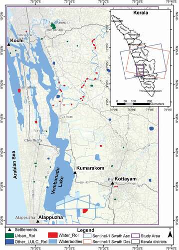
Figure 2. Methodology showing flood area mapping using EO images

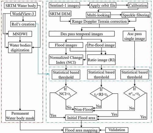
Figure 3. The sub-figures (a) show the PWB mask obtained by the proposed approach and (b) shows the PWB mask obtained by the JRC GSW layer. The sub-figure (c) shows the random points overlaid on the PWB obtained by the proposed approach

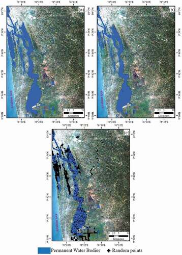
Figure 4. Statistical analysis of water, urban and other land use classes ROIs obtained from temporal indices (a) NCI and (b) RI

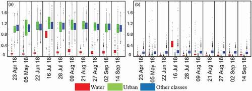
Figure 5. Change detection-based flood area plotted against IMD rainfall

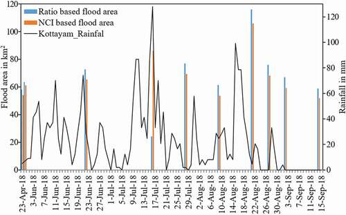
Figure 6. Change detection based flood maps obtained from pre-flood images. The figures (a), (b), (c) are the enlarged part of the rectangles shown in the left figures, but with SAR image as background. The rectangles are overlaid on Sentinel-2 true colour image on the top row and Open Street MAP (OSM) at the other rows

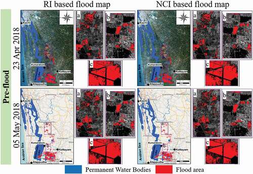
Figure 7. Change detection based flood maps obtained with pre-flood and during flood images. The figures (a), (b), (c) are the enlarged part of the rectangles shown in the left figures, but with SAR image as background. The rectangles are overlaid on Sentinel-2 true colour image on the top row and Open Street MAP (OSM) at the other rows

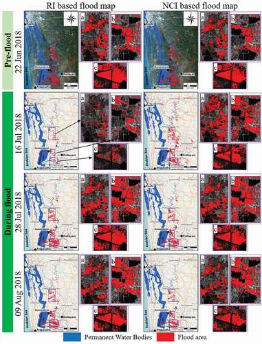
Figure 8. Change detection based flood maps obtained with during flood and post-flood images. The figures (a), (b), (c) are the enlarged part of the rectangles shown in the left figures, but with SAR image as background. The rectangles are overlaid on Sentinel-2 true colour image on the top row and Open Street MAP (OSM) at the other rows

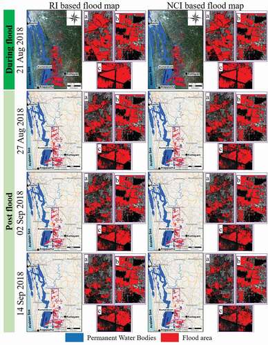
Figure 9. Flood area extracted from a single SAR image using the threshold method. The figures (a) and (c) are characterized mostly by agricultural land uses. Figure (b) is characterized by mixed land uses (buildings, roads, trees, open areas). The rectangles are overlaid on Sentinel-2 true colour image

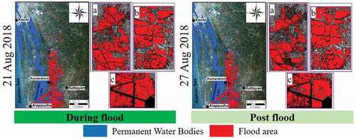
Figure 10. Temporal dynamics of land surface condition for a zoomed-in portion (b). Pre, During and Post indicated the images acquired on pre-flood, during flood, and post-flood. Plot-1 and Plot-2 show the agricultural areas

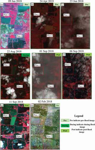
Figure 11. Flood area (excluding common area) extracted from both ascending and NCI images. The figures (a), (b), (c) are the enlarged part of the rectangles shown in the left figures. The rectangles are overlaid on Open Street MAP (OSM) layer

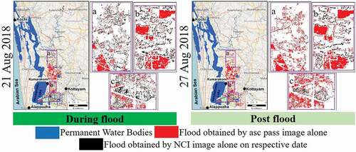
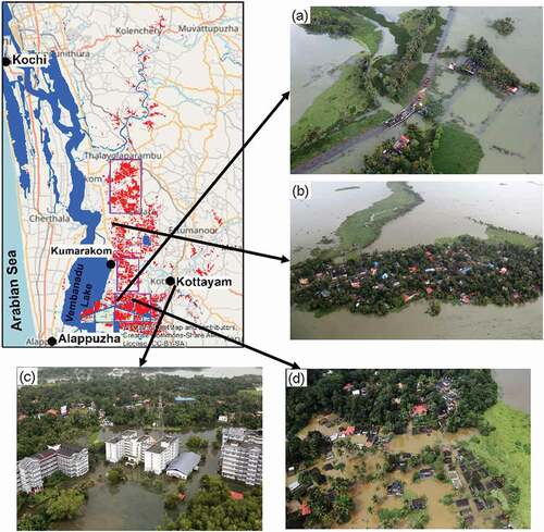
Figure 12.. (a), (b), (c), (d) shows an aerial view that has partially submerged houses on a flooded area located in and around Alappuzha and Kottayam districts

Datasets

Both optical (Worldview-3, Sentinel-2) and SAR (Sentinel-1) images are used to analyze the 2018 flood event of Kerala, India. To understand the flood progression and recession, the multi-temporal Level-1 Ground Range Detected (GRDH) Sentinel-1 SAR images that are acquired before, during and after the heavy rainfall are used. The Sentinel data can be obtained from Copernicus Open Access Hub (European Space Agency, 2018). The characteristics of optical and SAR images used in the study are described in Table 1 and the corresponding images are given in supplementary file Figures S1-S4.

Table 1. EO satellite images used for Kerala flood mapping occurred in 2018

Date of acquisition	Satellite	Acquisition mode/swath	Polarization/Bands	Pass	Flood condition
5 January 2018	Sentinel – 1	IW1 & IW2	VV	Des	Pre-flood
23 April 2018	Sentinel – 1	IW1 & IW2	VV	Des	Pre-flood
5 May 2018	Sentinel – 1	IW1 & IW2	VV	Des	Pre-flood
22 June 2018	Sentinel – 1	IW1 & IW2	VV	Des	Pre-flood
16 July 2018	Sentinel – 1	IW1 & IW2	VV	Des	During-flood
28 July 2018	Sentinel – 1	IW1 & IW2	VV	Des	During-flood
9 August 2018	Sentinel – 1	IW1 & IW2	VV	Des	During-flood
21 August 2018	Sentinel – 1	IW1 & IW2	VV	Des	During-flood
21 August 2018	Sentinel – 1	IW1 & IW2	VV	Asc	During-flood
27 August 2018	Sentinel – 1	IW1 & IW2	VV	Des	Post-flood
27 August 2018	Sentinel – 1	IW1 & IW2	VV	Asc	Post-flood
2 September 2018	Sentinel – 1	IW1 & IW2	VV	Des	Post-flood
14 September 2018	Sentinel – 1	IW1 & IW2	VV	Des	Post-flood
1 February, 21 February, 9 March, 27 April, and 12 July 2018	World View - 3	Nadir	B2/B3/B5	-	Pre-flood
14 January 2018	Sentinel-2	Nadir	B2/B3/B4	-	Pre-flood

Based on the flood condition, these temporal SAR images are divided into three categories. Images acquired on 5 January2018, 23 April 2018, 5 May 2018, and 22 June 2018 are categorized as pre-flood images. While the images acquired on 16 July 2018, 28 July 2018, 9 August 2018, and 21 August 2018 are categorized as during flood images. The images acquired on 27 August 2018, 02 September 2018, 14 September 2018 are categorized as post-flood images. In addition to the SAR images, the WorldView-3 optical images acquired before flood event are used to map the permanent water bodies. The WorldView-3 images are obtained from DigitalGlobe under the open data program from the link (DigitalGlobe, 2018). Also, permanent water bodies derived by STRM mission which are available from USGS Earth Explorer are also used in the creation of Permanent Water Body (PWB) mask in the study area extent. Sentinel-2 and secondary data such as field photographs are used for validation purpose. The rainfall datasets are obtained from the IMD website (Indian Meteorological Department, 2018).

Methodology

The overall methodology adopted for mapping the 2018 flood event of Kerala is shown in Figure 2. It is broadly divided into five modules, i.e. data pre-processing, PWB mask creation, training dataset creation and flood mapping techniques and CD indices. The first module describes the pre-processing of freely available C-band temporal Sentinel-1 SAR images and WorldView-3 optical image. The second module describes the PWB mask creation using both optical and SAR images. The third module describes the creation of training dataset, which plays a significant role in threshold identification. The fourth module describes the use of single date/temporal SAR images acquired in ascending/descending pass in flood identification through different flood mapping techniques. The last module elucidates the procedure of creating CD indices. The PWB mask’s accuracy is verified using the standard water body, i.e., Global Surface Water (GSW) layer created by the Joint Research Centre (JRC). Five hundred random points were generated from the GSW layer and overlaid on the PWB mask, as shown in Figure 3. The count of random points within and outside the PWB mask is generated with the help of geoprocessing tools. The PWB mask layer created in this study is found to be 99.14% accurate.

Data pre-processing

The Sentinel-1 SAR images are pre-processed in Sentinel Application Platform (SNAP) software provided by the European Space Agency (ESA). Various pre-processing steps viz., radiometric calibration, multi-looking, speckle filtering, and geometric calibration are implemented on level-1 temporal Ground Range Detected (GRDH) products. Multiple operators available in SNAP software like “Apply Orbit File”, “S1 Remove GRD Border Noise”, “Calibrate”, “Multilooking”, “Single Product Speckle Filter”, “Range-Doppler Terrain Correction”, “Subset” are used in pre-processing of SAR images. The orbit state vectors which defines the satellite position and velocity while acquiring the images are updated using the “Apply Orbit File” operator. The border noise present in the GRDH images is removed by “S1 Remove GRD Border Noise” operator. Subsequently, radiometric correction, i.e. conversion of pixel DN values to radar backscatter (σ°) values of the reflecting surfaces is performed. The calibrated images are multi-looked by 3 × 3 looks in azimuth and range directions, respectively. To reduce the speckle noise, gamma map filter with 3 × 3 is implemented on the multi-looked images. Further, geometric correction is performed on speckle filtered images to geocode the SAR images that are free from geometric distortions using “Range-Doppler Terrain Correction” operator. The terrain corrected images are in linear scale with a pixel size of 30 m x 30 m. All the temporal terrain corrected GRDH images are subset to the study area extent and used for further analysis.

As multiple images need to be processed in the same procedure, bulk processing is carried out in Sentinel Application Platform (SNAP) Graph Processing Framework (GPF) to automate the tasks. To this end, an XML code is created using the “Read”, “Output” and above mentioned GPF operators. The XML code is executed through the SNAP command line. The WorldView-3 optical images are pre-processed to derive the reflectance, which in turn used to digitize the permanent water bodies.

Permanent Water Body (PWB) mapping

In the flood area estimation, the permanent water bodies need to be masked out to deal with overestimation. Therefore, the PWB mask was created using two data sources, i.e., optical (World View) and SAR (Sentinel-1) datasets. Among the temporal Sentinel-1 SAR images, the 5 January 2018 SAR image was selected to map the major water bodies. This image was chosen because the land surface condition on that acquisition date was neither affected by soil moisture nor rainfall. During the pre-processing of this GRDH image, in the “Range-Doppler Terrain Correction” operator an option to mask out areas without elevation was chosen. The SRTM 3 sec DEM was used as an input in the terrain-correction process which has no elevation values for the major water bodies.

Subsequently, after the terrain correction, the radar backscatter coefficient σ° for the large water bodies and major river network were represented with a constant value (NaN). With the help of band math operator in SNAP, an expression σ°_vv = = NaN was created such that all the pixel values satisfying this condition were considered as PWB mask pixels. With respect to this, only the Vembanad lake, a major water body which is a RAMSAR recognized site, was highlighted. The PWB mask identified through SAR image in raster format was vectorized and converted it to a shapefile. However, due to the limitation of resolution and side looking nature of SAR datasets, the narrow water stream networks were not identified. A Normalized Difference Water Index (NDWI) was developed from green and IR bands of high-resolution optical RS images, i.e., WorldView images. Subsequently, manual digitization was carried out on NDWI to map the narrow water stream networks in the form of a shapefile. Finally, both optical and SAR-based shapefiles were merged to get a PWB mask.

Creation of training dataset

A training dataset is required to generate the optimum threshold for flood identification. So, the training dataset for various land cover (water bodies, vegetation, urban, and rural areas) is created by manual digitization on the WorldView-3 images. The Region of Interest (ROI) samples in the training dataset are carefully chosen over different land uses such that they are distributed throughout the study area. This ensures that the radar backscatter values from heterogeneous land uses are considered in optimum threshold identification. These multiple ROIs are superimposed on the SAR imagery for statistical analysis as shown in Figure 1. All the land cover classes except water bodies and urban areas are combined and labelled as other classes for ease of classification. The number of pixels per land cover class in the training dataset is 1483 (1.33 km²), 844 (0.75 km²), 2159 (1.94 km²) for water bodies, urban and other classes, respectively.

Flood mapping by ascending and descending pass SAR images

The semi-automatic approaches used in this study include either thresholding or CD techniques combined with thresholding for flood mapping. The potential of SAR images acquired during the flood with and without pre-flood image is explored for flood identification and quantification. During the Kerala flood, Sentinel-1 satellite acquired the images in both ascending and descending pass directions. The CD techniques apply only to the images acquired in descending pass direction due to the availability of pre-flood SAR images with the same image characteristics as the flood images. Since there are no pre-flood SAR images acquired in ascending pass direction, a threshold is selected by backscatter analysis of various land cover ROIs for flood area mapping.

For the images acquired in descending pass direction, the CD techniques such as ratio, and NCI combined with thresholding are used to generate the flood area and analyzed both spatially and quantitatively. For both techniques, the terrain corrected co-polarized (VV) σ°_vv images in linear scale are used. The selection of the pre-flood image to be used in the CD techniques is made in such a way that the image is not affected by rainfall. Also, it is ensured that there is little/no water in the study area, especially in the paddy fields at the image acquisition. From the temporal backscatter analysis, it is found that the image acquired during 5 January 2018 is more suitable as the pre-flood image. To understand the temporal pattern (increasing and receding) of flooding in the study area, all other images are treated as flood images. The temporal indices for both the CD techniques are generated. Subsequently, an optimum threshold is required to identify the flood area for which the indices are taken on a linear scale. The initial flood area obtained by these two techniques is refined by removing the permanent water bodies using PWB mask to minimize the overestimation errors.

Generation of Change Detection (CD) indices

All the temporal terrain corrected σ° images are co-registered in order to identify the change on the land surface. The changes will be detected on a pixel-by-pixel basis. During the co-registration, the 5 January 2018 image is chosen as the master image without any resampling. The number of GCP’s used in cross-correlation is 2000, and 0.05 RMS threshold (pixel accuracy) is used in the warping process. After the co-registration, all the temporal images are spatially aligned with 5 January 2018 image.

The Normalized change Index (NCI) is generated by normalizing the absolute difference between the flood and pre-flood images σ° values as given in Eq. 1(1) $NCI=\frac{{\sigma }_{vv\left(flood\right)}^0-{\sigma }_{vv\left(pre-flood\right)}^0}{{\sigma }_{vv\left(flood\right)}^0+{\sigma }_{vv\left(pre-flood\right)}^0}+1$(1) .

(1) $NCI=\frac{{\sigma }_{vv\left(flood\right)}^0-{\sigma }_{vv\left(pre-flood\right)}^0}{{\sigma }_{vv\left(flood\right)}^0+{\sigma }_{vv\left(pre-flood\right)}^0}+1$(1)

where σ°_vv(flood) = flood image Backscattering Coefficient (BSC) of VV polarization and σ°_{vv(pre-flood)} = pre-flood image (5 January 2018) BSC of VV polarization. The NCI values lie between 0 and 2, where the NCI value of 1 represents no change in both the images. The positive change in the NCI values represents the flood areas. The image acquired on 5 January 2018 was used as the pre-flood image for generating all the temporal NCI indices using the Eq. 1(1) $NCI=\frac{{\sigma }_{vv\left(flood\right)}^0-{\sigma }_{vv\left(pre-flood\right)}^0}{{\sigma }_{vv\left(flood\right)}^0+{\sigma }_{vv\left(pre-flood\right)}^0}+1$(1) . A bi-modal histogram is observed from the NCI image generated by pre-flood and peak flood images, i.e. 5 January and 21 August 2018 images, respectively. This is due to the presence of permanent water bodies and flood areas.

The Ratio Image (RI) is generated by taking the ratio of absolute values of flood image to the pre-flood image σ° values as given in Eq. 2(2) $RI=\frac{{\sigma }_{vv\left(flood\right)}^0}{{\sigma }_{vv\left(pre-flood\right)}^0}$(2) .

(2) $RI=\frac{{\sigma }_{vv\left(flood\right)}^0}{{\sigma }_{vv\left(pre-flood\right)}^0}$(2)

where σ°_vv(flood) = flood image BSC of VV polarization and σ°_{vv(pre-flood)} = pre-flood image (5 January 2018) BSC of VV polarization. The changes occurred over the land surface due to flooding can be seen if the RI << 1 (draw off) and RI >> 1 (infilling). The histogram for the RI image obtained by pre-flood and peak flood image, i.e. 5 January and 21 August 2018 is similar to the NCI. All the temporal RI indices are generated with a fixed pre-flood image (5 January 2018) using the Eq. 2(2) $RI=\frac{{\sigma }_{vv\left(flood\right)}^0}{{\sigma }_{vv\left(pre-flood\right)}^0}$(2) . To maintain the consistency among the temporal indices and to compare with NCI indices, all the temporal RI indices are normalized and scaled to the same data range of NCI indices.

Results

The results are grouped into two parts. The first part describes the threshold identification for flood area mapping, while the second part deals with flood area mapping from ascending pass SAR images.

Flood mapping by descending pass temporal SAR images

After generating the temporal RI and NCI indices, an optimal threshold was required to identify the flood area. The pixel values of all the ROIs, i.e. water, urban and other classes were extracted from the temporal CD indices, as shown in Figure 4.

In this figure, the X-axis represents image acquisition dates, whereas Y-axis represents the index values. The boxplots represent the pixel values for the respective thematic classes. From Figure 4, it was observed that the range of water class pixels was clearly separated from all other classes among temporal NCI images rather than RI images. From the statistical analysis of the indices, it is found that the range of pixel values is varying from 0.013 to 0.5 for RI, whereas 0.02 to 0.95 for NCI in case of water class. Among both indices, there was a sudden increase in the response from water class for the image acquired on 16 July 2018. This phenomenon can be understood from Figure 5 as it was the result of strong backscatter due to Bragg scattering obtained from flowing water in the river channel and also due to the presence of floodwater. The thresholds are identified carefully keeping this in view.

(3) ${\mu }_{water}=\frac{1}{N}\sum _{i=1}^{N}WaterRO{I}_i$(3)

(4) ${\sigma }_{water}=\sqrt{\frac{1}{N-1}\sum _{i=1}^N{\left|WaterRO{I}_i-{\mu }_{water}\right|}^2}$(4)

where N refers to the number of samples in the water ROI. µ_water, µ_urban refers to mean of water, urban pixel values and σ_water refers to the standard deviation of water pixel values.

From Eq. 3(3) ${\mu }_{water}=\frac{1}{N}\sum _{i=1}^{N}WaterRO{I}_i$(3) and 4(4) ${\sigma }_{water}=\sqrt{\frac{1}{N-1}\sum _{i=1}^N{\left|WaterRO{I}_i-{\mu }_{water}\right|}^2}$(4) , a threshold of (µ_water + σ_water) which is 0.4 is chosen for flood identification with temporal NCI indices. So, all the pixel values that are below this threshold are identified as a flood area. In the case of RI, the urban class pixels are also present within the threshold of (µ_water + σ_water) which is 0.1. Therefore, the threshold of the urban class is also calculated by (µ_urban + σ_urban), which is 0.04. Finally, the pixels that are lying between 0.04 and 0.1 are considered as flood area for temporal RI indices. The approach used for identifying the optimum thresholds for flood mapping in this study is robust. It can be universally applicable to any other flood events since threshold values are obtained by statistical analysis implemented on CD indices of various thematic land use classes (Krishna Vanama & Rao, 2019; Martinis et al., 2011; Yulianto et al., 2015). Also, this approach can be scalable to a larger spatial extent with minimal user inputs. The permanent water bodies are also classified as a flood area in the initial flood mapping process. Therefore, the initial flood area is refined by masking out the permanent water bodies. A post-processing approach is carried out on the refined flood layer for generating the binary flood maps (flood and non-flood). Post-processing includes the implementation of morphological filters like clump, sieve and re-coding the flood images as binary output. Finally, raster to vector conversion tool is used to generate the flood area in vector format. The spatial extent of flood area obtained by CD techniques combined with thresholding for pre, during, and post-flood images are shown in Figures 6, Figures 7 and Figures 8.

Three zoomed-in portions (a), (b), (c) that covers various land cover features are selected and given on the right side of the figure. Agricultural areas are covered in (a) and (c) regions. Mixed land uses, i.e. buildings, roads, trees, open areas are shown in (b) zoomed-in portion. The flood area and the permanent water bodies are represented in red and blue colours. The total amount of flood area obtained from the CD techniques combined with thresholding is shown in Figure 5.

Flood mapping by ascending pass single SAR image

After pre-processing the ascending pass Sentinel-1 SAR images, a backscattering analysis of various land cover classes is performed on VV polarized flood image (21 August 2018). From the backscatter analysis, it is found that water bodies, flooded regions, and wetlands areas are exhibiting similar backscatter responses. Therefore, a threshold of (µ_water + σ_water) which is 0.03 is found to be optimum for delineating the flood areas. All the pixels that are below this threshold value are considered as flooded. The same threshold is applied on post-flood ascending pass image acquired on 27 August 2018. The flood area obtained from this thresholding method includes permanent water bodies. Therefore, the permanent water bodies are masked out using PWB mask from the initial flood area to minimize the overestimation. Post-Processing is applied to the resultant flood area similar to the flood area detected from the descending pass images. The spatial extent of the flood area obtained from both ascending pass images is shown in Figure 9.

In the figures, the blue colour represents the permanent water bodies, and the red colour represents the flood area. The (a), (b), (c) represents the zoomed-in portion of Figure 9. The total flood area obtained for 21 August and 27 August 2018 images are 147.5 km², and 141.1 km² respectively. It is observed that the flood area has reduced from 21 August to 27 August 2018.

Discussions

The results of the quantitative analysis of flood area are similar to spatial analysis. From Figure 5, it is observed that an increasing trend in the flood area is seen during 21 August, followed by a subsequent receding trend. The flood area obtained from the pre-flood images is almost as same as post-flood images, which shows the land surface has regained its original position by September 2018. The second-highest spike in the flood area is observed on 16 July 2018. This is due to heavy rainfall occurred during 15 July and 16 July 2018, which led to the land surface being flooded. Among the two indices, NCI captured the actual flood area whereas RI underestimates it because RI is calculated merely by taking the ratio of absolute values. The flood area obtained from RI is higher than the NCI except for 16 July 2018. This indicates that there is a possibility that RI either overestimates or underestimates the flood area. It also implies that the performance of NCI in flood identification is better than RI since it is normalizing the difference between pre and flood image σ° values.

In the zoomed-in portion (b), some plots of the agricultural fields are not considered as flooded area as shown in Figure 6, Figures 7, Figures 8 by CD combined with thresholding technique applied on descending pass SAR images. But, they are considered as the flooded area by thresholding technique applied on ascending pass SAR images as shown in Figure 9. The former technique uses a pre-flood image and identifies the drastic changes that occurred on the land surface. Agricultural fields gave low backscattering values in both pre and during flood images due to specular reflection, due to which the changes occurring on the land surface were minimal. Therefore, they are not considered flooded by the former technique. This shows that CD techniques may lead to underestimation of flood area calculation in vegetation land cover if the land surface condition of the pre-flood image is not completely dry. This is possibly one of the reasons for the difference obtained in the flood area calculation among the two techniques. To understand the temporal land surface condition of a zoomed-in portion (b), False Color Composite (FCC) maps from Sentinel-2 images, and natural colour composite from WorldView-3 is shown in Figure 10. In Figure 10, plot-1 and plot-2 show the agricultural areas. (a) to (g) images are formed by Sentinel-2 FCCs and (h) is formed by WorldView-3 natural colour composite.

The zoomed-in portion (a) consist of water like radar response features such as roads, open land area, and river channel, which may lead to overestimation. The open land area and river channel are considered as the flooded area, as shown in Figure 9 by the thresholding technique applied on ascending pass SAR images. This is very prominently visible on the post-flood image acquired on 27 August 2018 where the floodwater is receding. But, they are not considered as flooded area as shown in Figure 8 by CD combined with thresholding technique applied on descending pass SAR images. The latter technique uses a pre-flood image in flood identification which minimizes the overestimation. So, it can be inferred that the use of the pre-flood image can enhance the flood area identification spatially among water like radar response features.

For the further understanding of the temporal dynamics of the flood, the combined use of ascending and descending pass images available on the same date in flood identification is explored. The flood area obtained from both the ascending and descending pass images is combined, as shown in Figure 11 for 21 August and 27 August 2018. In Figure 11, the common flood area in both ascending and descending pass images is omitted as it is detected from both techniques. The red colour area shows the flood area obtained from the ascending pass image based on thresholding alone whereas the black colour shows the flood area obtained from the descending pass image based on NCI combined with thresholding on respective dates. The flood area from both ascending and descending pass images after omitting the common area is overlaid on the Google earth. It is identified that various land cover features such as buildings, roads, open areas and vegetation got flooded. Even though the flood water started receding from 21 August 2018, the agricultural fields in the zoomed-in portions (a), (b), and (c) are considered as flooded by thresholding technique applied on ascending pass image acquired on 27 August 2018. This is due to the fact that the agricultural fields gave low backscattering values which are in the range of water bodies backscattering values.

Apart from the strengths and weakness of the flood mapping techniques, other parameters such as acquisition time, look direction, orientation also play a significant role in the identification of flood area. In the case of Kerala flood, there is a time difference of 12 hrs between the image acquisition of ascending and descending pass images. Therefore, it is possible that the flood water may start receding to the Vembanad lake. Also, the objects which are oriented perpendicular and parallel to the line of sight result in high and low backscatter values. In the zoomed-in portions (c) some plots of the agricultural fields are oriented from near parallel to near perpendicular to the line of sight in both ascending and descending pass directions. The above two factors are some of the reasons for the mismatch of flood area obtained from ascending and descending pass images.

For validation purpose, the results are plotted against the rainfall data obtained from the CWC report and IMD data, as shown in Figure 5. As per the CWC report, the total flood area estimated for the two entire districts, i.e. Kottayam and Alappuzha from 15 August to 27 August 2018 is 480 km². The study area of this research is only a part of these two districts. Therefore, the flood area obtained from our methods doesn’t match with the CWC quantitative flood estimates. The spatial extent of the flood area obtained by our methods is almost similar to the flood area given in ISRO Bhuvan Near Real-Time Flood Monitoring web portal and NRSC estimates (NRSC, 2018). Also, due to heavy rainfall, the communication and transportation facilities are halted for more than a month. In this scenario, conducting a manual survey on such a large area is quite difficult. Also, this survey requires enormous resources such as skilled labour, financial, and computational resources. Therefore, the geotagged photographs that were captured during the flood are obtained from various open-source blogs (Reuters, 2018). The ground coordinates of photos are superimposed on the flood area and found that their locations are within their bounds as shown in Figure 11Figure 12.

Conclusion

The launch of the C-band Sentinel satellite has revolutionized the use of SAR images in various applications majorly due to the freely available dual-pol temporal images. With the upcoming SAR missions like NASA-ISRO Synthetic Aperture Radar (NISAR), TerraSAR-L, Biomass, and Capella X-SAR, the usage of SAR data for flood mapping have increased manyfold. In this study, the potential of freely available multi-temporal EO images in flood mapping was demonstrated for 2018 Kerala flood event. During the time of disasters, image acquisitions depend entirely on the availability of satellite passes. Typically, Sentinel-1 acquires images in descending pass direction for southern India at a temporal resolution of 12 days. Acquiring two images on the same day with a temporal resolution of 6 days by a constellation of satellites to monitor a flood disaster event is a rare scenario. During the Kerala flood, two images were acquired in ascending and descending pass directions on the same day. Sentinel-1A acquired two images on 21 August 2018, and Sentinel-1B acquired two images on 27 August 2018. As flood is a dynamic phenomenon, such acquisitions if possible can greatly benefit the monitoring and mapping of a flood event. Therefore, this study explores this scenario for assessing the combined use of ascending and descending pass satellite images over the same location on the same date to monitor the flood progression and recession in the duration of a flood event.

Two simple and reliable semi-automatic approaches, i.e. statistical-based thresholding and CD techniques combined with thresholding were implemented on temporal SAR images. From the results, it can be concluded that among the two CD techniques, NCI outperformed the RI for Kerala flood event. It is also noted that CD techniques may lead to underestimation if a proper pre-flood image is not selected without considering the seasonality/land surface condition. The results also highlight the utility of the pre-flood image in handling the overestimation of the flood area. In addition, this study demonstrated the PWB creation with high-resolution optical and SAR images. The thresholding approach used in this study is universally applicable. However, this approach is limited by the distribution of pixel values in the raw data. Henceforth, the end users are advised to check the data quality before implementing this approach. If there are any extremely low-value pixels in the data, they can be discarded before generating the CD indices. Additionally, this approach is also limited by the type of land surface exposed to flooding, and this approach performs well for rural, urban, and semi-urban land uses. In case the flood happens in a dense forest region, this approach can be slightly modified by considering (µ + 2σ) for thresholding identification, due to the low penetration of C-band in the forest region. The findings of this study can be useful for flood mitigation measures and the preparation of contingency plans for future flood events. This study can be further extended by developing automatic algorithms on cloud computing platforms such as Google Earth Engine (GEE).

Table 1: EO satellite images used for Kerala flood mapping occurred in 2018

Acknowledgement

The first author is thankful to the Ministry of Human Resource Development (MHRD), GoI for providing necessary computational facilities through the project (14MHRD005) funding. The authors would like to thank DigitalGlobe for providing the high-resolution WorldView-3 images and ESA for providing Sentinel-1 through Copernicus Open Access Hub.

Disclosure statement

No potential conflict of interest was reported by the authors.

Correction Statement

This article has been republished with minor changes. These changes do not impact the academic content of the article.

References

- Amarnath, G. (2014). An algorithm for rapid flood inundation mapping from optical data using a reflectance differencing technique: Rapid flood inundation mapping algorithm. Journal of Flood Risk Management, 7(3), 239–250. https://doi.org/https://doi.org/10.1111/jfr3.12045
- Baghdadi, N., Bernier, M., Gauthier, R., & Neeson, I. (2001). Evaluation of C-band SAR data for wetlands mapping. International Journal of Remote Sensing, 22(1), 71–88. https://doi.org/https://doi.org/10.1080/014311601750038857
- Behera, M. (2008). Kerala Floods Joint Detailed Needs Assessment Report. National coalition of humanitarian agencies in India. (pp. 1–66) https://ndma.gov.in/images/guidelines/flood.pdf
- Bonn, F., & Dixon, R. (2005). Monitoring Flood Extent and Forecasting Excess Runoff Risk with RADARSAT-1 Data. Natural Hazards, 35(3), 377–393. https://doi.org/https://doi.org/10.1007/s11069-004-1798-1
- Brisco, B., Schmitt, A., Murnaghan, K., Kaya, S., & Roth, A. (2013). SAR polarimetric change detection for flooded vegetation. International Journal of Digital Earth, 6(2), 103–114. https://doi.org/https://doi.org/10.1080/17538947.2011.608813
- Central Water Commission, I. (2018). Study Report: Kerala Flood of August 2018. Central Water Commission, Hydrological Studies Organisation. (September; pp. 1–46).
- Chaouch, N., Temimi, M., Hagen, S., Weishampel, J., Medeiros, S., & Khanbilvardi, R. (2012). A synergetic use of satellite imagery from SAR and optical sensors to improve coastal flood mapping in the Gulf of Mexico. Hydrological Processes, 26(11), 1617–1628. https://doi.org/https://doi.org/10.1002/hyp.8268
- Chini, M., Hostache, R., Giustarini, L., & Matgen, P. (2017). A Hierarchical Split-Based Approach for Parametric Thresholding of SAR Images: Flood Inundation as a Test Case. IEEE Transactions on Geoscience and Remote Sensing, 55(12), 6975–6988. https://doi.org/https://doi.org/10.1109/TGRS.2017.2737664
- Chini, M., Pelich, R., Pulvirenti, L., Pierdicca, N., Hostache, R., & Matgen, P. (2019). Sentinel-1 InSAR Coherence to Detect Flood water in Urban Areas: Houston and Hurricane Harvey as A Test Case. Remote Sensing, 11(2), 107. https://doi.org/https://doi.org/10.3390/rs11020107
- Chung, H.-W., Liu, -C.-C., Cheng, I.-F., Lee, Y.-R., & Shieh, M.-C. (2015). Rapid Response to a Typhoon-Induced Flood with an SAR-Derived Map of Inundated Areas: Case Study and Validation. Remote Sensing, 7(9), 11954–11973. https://doi.org/https://doi.org/10.3390/rs70911954
- Cian, F., Marconcini, M., & Ceccato, P. (2018). Normalized Difference Flood Index for rapid flood mapping: Taking advantage of EO big data. Remote Sensing of Environment, 209, 712–730. https://doi.org/https://doi.org/10.1016/j.rse.2018.03.006
- Cleve, C., Kelly, M., Kearns, F. R., & Moritz, M. (2008). Classification of the wildland–urban interface: A comparison of pixel- and object-based classifications using high-resolution aerial photography. Computers, Environment and Urban Systems, 32(4), 317–326. https://doi.org/https://doi.org/10.1016/j.compenvurbsys.2007.10.001
- De Groeve, T. (2010). Flood monitoring and mapping using passive microwave remote sensing in Namibia. Geomatics, Natural Hazards and Risk, 1(1), 19–35. https://doi.org/https://doi.org/10.1080/19475701003648085
- Dewan, A. M., Kankam-Yeboah, K., & NISHIGAKI, M. (2006). Using Synthetic Aperture Radar (SAR) Data for Mapping River Water Flooding in an Urban Landscape: A Case Study of Greater Dhaka, Bangladesh. Journal of Japan Society of Hydrology and Water Resources, 19(1), 44–54. https://doi.org/https://doi.org/10.3178/jjshwr.19.44
- DigitalGlobe. (2018). Open Data Program—Flooding in India. https://www.digitalglobe.com/opendata/flooding-in-india/pre-event
- European Space Agency. (2018). Copernicus Open Access Hub. https://scihub.copernicus.eu/dhus/#/home
- Giustarini, L., Hostache, R., Kavetski, D., Chini, M., Corato, G., Schlaffer, S., & Matgen, P. (2016). Probabilistic Flood Mapping Using Synthetic Aperture Radar Data. IEEE Transactions on Geoscience and Remote Sensing, 54(12), 6958–6969. https://doi.org/https://doi.org/10.1109/TGRS.2016.2592951
- Giustarini, L., Hostache, R., Matgen, P., Schumann, G. J. P., Bates, P. D., & Mason, D. C. (2013). A Change Detection Approach to Flood Mapping in Urban Areas Using TerraSAR-X. IEEE Transactions on Geoscience and Remote Sensing, 51(4), 2417–2430. https://doi.org/https://doi.org/10.1109/TGRS.2012.2210901
- Greifeneder, F., Wagner, W., Sabel, D., & Naeimi, V. (2014). Suitability of SAR imagery for automatic flood mapping in the Lower Mekong Basin. International Journal of Remote Sensing, 35(8), 2857–2874. https://doi.org/https://doi.org/10.1080/01431161.2014.890299
- Guo, H.-D., Zhang, L., & Zhu, L.-W. (2015). Earth observation big data for climate change research. Advances in Climate Change Research, 6(2), 108–117. https://doi.org/https://doi.org/10.1016/j.accre.2015.09.007
- Henry, J.-B., Chastanet, P., Fellah, K., & Desnos, Y.-L. (2006). Envisat multi-polarized ASAR data for flood mapping. International Journal of Remote Sensing, 27(10), 1921–1929. https://doi.org/https://doi.org/10.1080/01431160500486724
- Hostache, R., Chini, M., Giustarini, L., Neal, J., Kavetski, D., Wood, M., Corato, G., Pelich, R.-M., & Matgen, P. (2018). Near-Real-Time Assimilation of SAR-Derived Flood Maps for Improving Flood Forecasts. Water Resources Research, 54(8), 5516–5535. https://doi.org/https://doi.org/10.1029/2017WR022205
- Huang, X., Tan, H., Zhou, J., Yang, T., Benjamin, A., Wen, S. W., Li, S., Liu, A., Li, X., Fen, S., & Li, X. (2008). Flood hazard in Hunan province of China: An economic loss analysis. Natural Hazards, 47(1), 65–73. https://doi.org/https://doi.org/10.1007/s11069-007-9197-z
- Indian Meteorological Department. (2018). Performance of South West Monsoon 2018 Over Kerala. Meteorological Centre. https://www.imdtvm.gov.in/images/cumulativerainfallforkerala-swmonsoon2018.pdf
- Jain, S. K., Saraf, A. K., Goswami, A., & Ahmad, T. (2006). Flood inundation mapping using NOAA AVHRR data. Water Resources Management, 20(6), 949–959. https://doi.org/https://doi.org/10.1007/s11269-006-9016-4
- Kiage, L. M., Walker, N. D., Balasubramanian, S., Babin, A., & Barras, J. (2005). Applications of Radarsat-1 synthetic aperture radar imagery to assess hurricane-related flooding of coastal Louisiana. International Journal of Remote Sensing, 26(24), 5359–5380. https://doi.org/https://doi.org/10.1080/01431160500442438
- Krishna Vanama, V. S., & Rao, Y. S. (2019). Change Detection Based Flood Mapping of 2015 Flood Event of Chennai City Using Sentinel-1 SAR Images. IGARSS 2019-2019 IEEE International Geoscience and Remote Sensing Symposium, 9729–9732. https://doi.org/https://doi.org/10.1109/IGARSS.2019.8899282
- Kundu, S., Aggarwal, S. P., Kingma, N., Mondal, A., & Khare, D. (2015). Flood monitoring using microwave remote sensing in a part of Nuna river basin, Odisha, India. Natural Hazards, 76(1), 123–138. https://doi.org/https://doi.org/10.1007/s11069-014-1478-8
- Ma, Y., Wu, H., Wang, L., Huang, B., Ranjan, R., Zomaya, A., & Jie, W. (2015). Remote sensing big data computing: Challenges and opportunities. Future Generation Computer Systems, 51, 47–60. https://doi.org/https://doi.org/10.1016/j.future.2014.10.029
- Manavalan, R. (2017). SAR image analysis techniques for flood area mapping - literature survey. Earth Science Informatics, 10(1), 1–14. https://doi.org/https://doi.org/10.1007/s12145-016-0274-2
- Manjusree, P., Prasanna Kumar, L., Bhatt, C. M., Rao, G. S., & Bhanumurthy, V. (2012). Optimization of threshold ranges for rapid flood inundation mapping by evaluating backscatter profiles of high incidence angle SAR images. International Journal of Disaster Risk Science, 3(2), 113–122. https://doi.org/https://doi.org/10.1007/s13753-012-0011-5
- Martinis, S., Twele, A., & Voigt, S. (2011). Unsupervised Extraction of Flood-Induced Backscatter Changes in SAR Data Using Markov Image Modeling on Irregular Graphs. IEEE Transactions on Geoscience and Remote Sensing, 49(1), 251–263. https://doi.org/https://doi.org/10.1109/TGRS.2010.2052816
- National Disaster Management Authority (2008). National Disaster Management Guidelines—Management of Floods. Publication of NDMA. (pp. 1–46)https://ndma.gov.in/images/guidelines/flood.pdf
- Nico, G., Pappalepore, M., Pasquariello, G., Refice, A., & Samarelli, S. (2000). Comparison of SAR amplitude vs. coherence flood detection methods - a GIS application. International Journal of Remote Sensing, 21(8), 1619–1631. https://doi.org/https://doi.org/10.1080/014311600209931
- NRSC. (2018). Flood Duration map of Part of Kerala State during 11-21st August 2018.
- Ohki, M., & Shimada, M. (2019). Flood Detection in Built-up Area Using Interferometric SAR Data by Palsar-2. IGARSS 2019-2019 IEEE International Geoscience and Remote Sensing Symposium, 4640–4642. https://doi.org/https://doi.org/10.1109/IGARSS.2019.8900344
- Ologunorisa, T. E., & Abawua, M. J. (2005). Flood risk assessment: A review. https://tspace.library.utoronto.ca/handle/1807/6419
- Panhalkar, S. S., & Jarag, A. P. (2017). Flood Risk Assessment of Panchganga River (Kolhapur District, Maharashtra) Using GIS-Based Multicriteria Decision Technique. Current Science, 112(4), 785. https://doi.org/https://doi.org/10.18520/cs/v112/i04/785-793
- Pelich, R., Chini, M., Hostache, R., Matgen, P., & López-Martínez, C. (2020). Coastline Detection Based on Sentinel-1 Time Series for Ship- and Flood-Monitoring Applications. IEEE Geoscience and Remote Sensing Letters, 1–5. https://doi.org/https://doi.org/10.1109/LGRS.2020.3008011
- Potin, P., Rosich, B., Miranda, N., Grimont, P., Bargellini, P., Monjoux, E., Martin, J., Desnos, Y.-L., Roeder, J., Shurmer, I., O’Connel, A., Torres, R., & Krassenburg, M. (2015). Sentinel-1 mission status. 2015 IEEE International Geoscience and Remote Sensing Symposium (IGARSS), 2820–2823. https://doi.org/https://doi.org/10.1109/IGARSS.2015.7326401
- Reuters. (2018). Floods in Kerala. https://in.reuters.com/news/picture/floods-in-kerala-idINRTS1XFOF
- Sheng, Y., Gong, P., & Xiao, Q. (2001). Quantitative dynamic flood monitoring with NOAA AVHRR. International Journal of Remote Sensing, 22(9), 1709–1724. https://doi.org/https://doi.org/10.1080/01431160118481
- Torres, R., Snoeij, P., Geudtner, D., Bibby, D., Davidson, M., Attema, E., Potin, P., Rommen, B., Floury, N., Brown, M., Traver, I. N., Deghaye, P., Duesmann, B., Rosich, B., Miranda, N., Bruno, C., L’Abbate, M., Croci, R., Pietropaolo, A., & Rostan, F. (2012). GMES Sentinel-1 mission. Remote Sensing of Environment, 120, 9–24. https://doi.org/https://doi.org/10.1016/j.rse.2011.05.028
- Twele, A., Cao, W., Plank, S., & Martinis, S. (2016). Sentinel-1-based flood mapping: A fully automated processing chain. International Journal of Remote Sensing, 37(13), 2990–3004. https://doi.org/https://doi.org/10.1080/01431161.2016.1192304
- Wang, Y., Ruan, R., She, Y., & Yan, M. (2011). Extraction of Water Information based on RADARSAT SAR and Landsat ETM+. Procedia Environmental Sciences, 10, 2301–2306. https://doi.org/https://doi.org/10.1016/j.proenv.2011.09.359
- Werle, D., Martin, T. C., & Hasan, K. (2000). Flood and coastal zone monitoring in Bangladesh with Radarsat ScanSAR: Technical experience and institutional challenges. Johns Hopkins APL Technical Digest, 21(1), 148–154. .semanticscholar.org/paper/Flood-and-Coastal-Zone-Monitoring-in-Bangladesh-and-Werle-Werle/d5a602326366e2a3cba51a1819a39ac845e06450
- White, L., Brisco, B., Pregitzer, M., Tedford, B., & Boychuk, L. (2014). RADARSAT-2 Beam Mode Selection for Surface Water and Flooded Vegetation Mapping. Canadian Journal of Remote Sensing, 40(2), 135–151. https://doi.org/https://doi.org/10.1080/07038992.2014.943393
- Yang, C., Huang, Q., Li, Z., Liu, K., & Hu, F. (2017). Big Data and cloud computing: Innovation opportunities and challenges. International Journal of Digital Earth, 10(1), 13–53. https://doi.org/https://doi.org/10.1080/17538947.2016.1239771
- Yulianto, F., Sofan, P., Zubaidah, A., Sukowati, K. A. D., Pasaribu, J. M., & Khomarudin, M. R. (2015). Detecting areas affected by flood using multi-temporal ALOS PALSAR remotely sensed data in Karawang, West Java, Indonesia. Natural Hazards, 77(2), 959–985. https://doi.org/https://doi.org/10.1007/s11069-015-1633-x