A review and meta-analysis of remote sensing data, GIS methods, materials and indices used for monitoring the coastline evolution over the last twenty years

ABSTRACT

The current review study focuses on a statistical analysis (Meta-analysis) of the most common methods, materials, software, and indices used by researchers over the last twenty years to evaluate and quantify the shoreline evolution. Furthermore, this review targets to highlight some critical points through studied literature such as a) the low rate of high-resolution satellite images usage in a subject where the accuracy is prerequisite, b) the effort to derive information from Landsat images in order to take advantage of the 50-years archive and the freely availability c) the impulse of the UAV during the last 5 years as an alternative low cost but high accurate source of data d) the fact that only 50% of the coastal erosion studies are funded. One hundred thirty-eight papers and articles have been analyzed in detail by the authors and all the key points (methods, materials, software, and indices) were sorted for further statistical analysis. This study is not intended to criticize neither the methods nor the results being mentioned in the previous studies but to give the opportunity to the researchers (especially the new ones) to have an overall view of the subject for the last 20 years with just a glimpse.

KEYWORDS:

• Meta-analysis
• gis
• remote sensing
• coastal erosion
• review

Introduction

About the shoreline

There are plenty of shoreline definitions along the time among researchers (Alesheikh et al., 2004; E Bird, 2008; Coastal Engineering Research Center (CERC), 1984; Niedermeier et al., 2005; Pajak & Leatherman, 2002). A conventional definition for the term “shoreline” is the physical border between land and sea (Dolan et al., 1980). The term “shoreline” is considered synonymous with the term “coastline” and there is no difference in this review study. During the last decades, the remote sensing science in combination with several Geographic Information System (GIS) applications has taken a various place in geo-surveys such as the coastline evolution analysis. Many studies tried to analyze and find the best approach to this subject based on several algorithms and computations (table 1–4). Automatic classification algorithms were also used and applied on aerial photos (A.C. Teodoro et al., 2009) or on IKONOS-2 satellite data (A. Teodoro et al., 2011) to identify coastal features and coastal patterns. The coastline is a dynamic environment where human structures and activities took place near or along it. So, it is important to have a reliable tool to enumerate, estimate and even, if so, to predict the shoreline movement landward or seaward. For this reason, many numeric methods, factors and algorithms have been established and applied the last two decades on a variety of data types such as aerial photos, satellite images, or Optical and RADAR data, Topographic maps and recently Unmanned Aerial Vehicle (UAV) images. The structure of the coastal environment and the pressures it is under are the first things that someone should understand in order to study its development. As coastline is a dynamic environment and it’s profile can very easily change from coast to coast continually, there is not one and only indicator which can match to all types of coasts. Indicators that measure the evolution and change of the coastline should be accurate and describe the timeless evolution of the area as well as the natural processes that have taken place. In figure 1 the allocation of diverse studies areas all over the world is presented. At these areas, shoreline evolution mapping was performed using remote sensing data/technologies as described in 138 studies published in the last 20 years (table 1–4).

Figure 1. Allocation of diverse studies areas regarding the application of remote sensing technology in shoreline evolution mapping

Table 1. Researchers’ whose interest about time interval (n) of shoreline monitoring was n ≤ 10 years

	Researchers	Place	Period of study	Years interval	Number of Citations
	Chao Chen et al. (Chen Chao Chen et al., 2019)	Yangtze River	2017	1	6
	Gudina et al. (Gudina Feyisa et al., 2014)	Copenhagen, Denmark, Switzerland, Addis Ababa, Ethiopia, South Africa, New Zealand	2009–2010	1	No data
	Ganasri and Ramesh (2016)	Nethravathi/India	2009	1	17
	Aiello et al. (Antonello et al., 2015)	Italy, CATENA	2001	1	77
	Papakonstantinou et al. (2016)	Lesvos Island, Eressos beach Greece	2015	1	3
	Chikhradze et al. (Nino et al., 2015)	Portugal	2015	1	No data
	Sekovski et al. (Ivan et al., 2014)	Ravenna Province Italy	2011	1	82
	Nikolakopoulos et al. (Nikolakopoulos Konstantinos & George, 2017)	Rio, Patras, Greece		1	79
	Nikolakopoulos et al. (Konstantinos et al., 2007)	Greece	2004	1	43
	Drummond et al. (Christopher et al., 2015)		2015	1	30
	Elsner et al. (Elsner Paul et al., 2015)	Pevensey Bay, East Sussex, England	2014	1	No data
	Letortu et al. (Pauline et al., 2018)	Dieppe, in Seine-Maritime, Normandy	2016	1	No data
	Nahon et al. (Alphonse et al., 2019)	Cap Ferret, SW France	2018	1	No data
	Paravolidakis et al. (2016)	Crete, Greece	2016	1	24
	Yan et al. (2019)	Caofeidian Port and the Xiamen china	2019	1	No data
	Modava et al. (Mohammad et al., 2018)	Panama Canal	2018	1	74
	Robertson et al. (2004)	USA Carolina State	2000	1	129
	Casella et al. (2016)	Ligurian Sea, Italy	2013–2014	1	33
	Mitra & et al. (Mitra et al., 2017)	Mandarmani coast	2009	1	90
	Turner et al. (Ian et al., 2016)	Narrabeen Beach southeast Australia	2015	1	29
	Al_Fugara et al. (2011)	Kuala Terengganu, Peninsular Malaysia	2005	1	25
	Valentini et al. (Nico et al., 2017)	Lecce, IT	2017	1	54
	Taha & Elbeih (LGEd & Elbeih, 2010)	Egypt Port Said	2000	1	31
	Zifeng et al. (2018)	Australia	2018	1	125
	Saravanan et al. (Sakthivel et al., 2014)	SE India	2000–2002	2	471
	Cooley & Barber (Cooley Paul & Barber David, 2003)	Lake Malawi, Africa	1996–1998	2	471
	Di et al. (2003)	Anchorage, Alaska	2000–2002	2	No data
	Benqing et al. (Benqing Chen et al., 2018)	China	2013–2014	2	No data
	Ratna et al. (2017)	Java Indonesia	2013–2015	2	1
	Duarte et al. (2018)	Port of Pecém Brazil	2011–2014	3	3
	Cabezas-Rabadán et al. (2019)	Gulf of Valencia, Spain	2015–2018	3	151
	Vandebroek et al. (2017)	Sand Motor Netherlands	2011–2014	3	18
	Gares et al. (Gares Paul et al., 2006)	Wrightsville Beach USA	1997–2000	3	16
	Marcaccio et al. (2015)	Southwestern Ontario	2010–2014	4	44
	Mörner and Klein (2017)	Yasawa Islands, Fiji	2005–2009	4	4
	Manjulavani et al. (2017)	Tuticorin coast India	2011–2015	4	8
	Kroon et al. (2007)	Netherlands/Italy and Spain	1998/1999/2003	5	58
	Nunziata et al. (2018)	Serapo and S. Agostino Thyrrenian Sea	2013–2018	5	15
	Davidson et al. (2010)	Gold Coast, Australia	2001–2006	5	150
	Al Mansoori & Al-Marzouqi (2016)	Dubai coastline	2009–2015	6	55
	Bruno et al. (2016)	Apulia Region (Italy)	2009–2015	6	82
	Mujabar et al. (2013)	Kanyakumari and Tuticorin of south India	1999–2006	7	457
	Maglione et al. (2015)	Campania coastal, Italy	2005–2012	7	84
	Mujabar and Chandrasekar (2013)	India	1999–2006	7	12
	Raju et al. (2015)	Mangalore India	2005–2013	8	159
	Senevirathna et al. (2018)	Sri Lanka	2007–2015	8	52
	Liu & Trinder (2018)	Gold Coast of Australia	1999–2008	9	No data
	Trebossen et al. (2005)	French Guiana	1992–2002	10	17

Table 2. Researchers’ whose interest about time interval (n) of shoreline monitoring was 10 < n ≤ 30 years

	Researchers	Place	Period of study	Years interval	Number of Citations
	Kaliraj et al. (2017)	Kanyakumari, South India	2000–2011	11	No data
	da Guia et al. (2013)	Hermenegildo Brazil	2000–2011	11	11
	Prasita (2015)	Pamurbaya/Indonesia	2002–2014	12	4
	Weicheng (2007)	Nouakchott, Mauritania	1989–2001	12	No data
	Grigio et al. (2005)	Guamaré City, Northeast Brazil	1989–2001	12	32
	Vanderstraete et al. (2006)	Hurghada, Egypt	1987–2000	13	11
	Shalaby & Tateishi (2007)	Northwestern Egypt	1987–2001	14	13
	Pantanahiran (2019)	Koh Kho Khao, Southern Thailand	2002–2016	14	10
	Shaghude et al. (2003)	Zanzibar	1986–2000	14	7
	Almonacid-Caballer et al. (2015)	El Saler (Valencia, Spain)	2000–2014	14	No data
	Chen & Hsien-Kuo (2009)	Wai-san-ting Chou, Taiwan	1993–2007	14	24
	Paravolidakis et al. (2018)	Crete, Greece	1990–2005	15	21
	Nageswara et al. (2008)	Andhra Pradesh coast, India	1990–2006	16	22
	Nan (2018)	Galveston, Texas	1986–2015	19	No data
	Shui-sen Chen et al. (2005)	South China	1978–1998	20	1
	Asib et al. (2018)	Bangladesh	1989–2010	21	32
	Kawakubo et al. (2011)	Icapara and Ararapira, Brazil	1986–2007	21	11
	Kankara et al. (2015)	Andhra Pradesh coast, east India	1990–2012	22	15
	Hegde & Akshaya (2015)	Karnataka India	1991–2014	23	110
	Vassilakis et al. (2016)	Corinthian Gulf	1987–2012	25	No data
	Petropoulos et al. (2015)	Thermaikos Gulf	1984–2009	25	No data
	Rasuly et al. (2010)	Caspian Sea	1977–2002	25	1
	Esmail et al. (2019)	Damietta coast, Egypt	1990–2015	25	29
	Majed et al. (2012)	Djerba, Tunisia	1984–2009	25	1
	Addo et al. (2011)	Keta, Ghana	1986–2011	25	8
	Do et al. (2018)	North-Holland from Wijk aan Zee to Den Helder	1985–2010	25	5
	Gormus et al. (2014)	Sakarya, Turkey	1987–2013	26	4
	Sandeep et al. (2018)	Bakkhali West Bengal, India	1990–2016	26	5
	Cenci et al. (2013)	Portugal Ovar and Marinha Grande	1984–2011	27	12
	Nassar et al. (2019)	North Sinai coast, Egypt	1989–2016	27	3
	Ratna (2019)	Semarang Java	1988–2017	29	11
	Qingxiang et al. (2017)	Narrabeen-Collaroy Beach, Australia	1987–2016	29	14
	Behling et al. (2018)	Namibia	1984–2014	30	33
	In-Ho et al. (2013)	Gonghyunjin and Songjiho Beaches, South Korea	1991–2010	30	No data
	Konko et al. (2018)	Togo (West Africa)	1988–2018	30	1
	Brock et al. (2001)	Balasore and Midnapur, India	1973–2003	30	0

Table 3. Researchers’ whose interest about time interval (n) of shoreline monitoring was 30 < n ≤ 70 years

	Researchers	Place	Period of study	Years interval	Number of Citations
	Thampanya et al. (2006)	Southern Thailand	1966–1997	31	No data
	Cenci et al. (2017)	Portugal (Ovar) Italy (Magra and Serchio)	1980–2011	31	17
	Sesli et al. (2008)	Trabzon, Turkey	1973–2005	32	No data
	Joevivek et al. (2018)	Tamil Nadu, India	1973–2006	33	2
	Joevivek et al. (2013)	Manavai and Vijayapathi, Southern Tip of India	1973–2006	33	1
	El-Asmar and Hereher (2011)	Nile Delta	1973–2007	34	No data
	Ratna et al. (2018)	Central Java Province, Indonesia	1988–2017	35	No data
	Ratna & Wietske (2019)	Sayung, Indonesia	1988–2017	35	2
	Liu et al. (2013)	Qingshuigou River, China	1973–2009	36	4
	Natesan et al. (2015)	Tamil Nadu, India	1978–2014	36	0
	Pardo-Pascual et al. (2012)	port of Borriana, Spain	1984–2010	36	No data
	Fatima et al. (2018)	Morocco	1981–2017	36	134
	Pritam & Prasenjit (2010)	Bhitarkanika, India	1973–2009	36	No data
	Xuejie and Damen (2010)	China	1966–2003	37	No data
	Kuleli et al. (2011)	Ramsar Turkey	1972–2009	37	21
	Bulent et al. (2004)	Istanbul	1963–2000	37	14
	Hashmi et al. (2018)	Sindh Pakistan	1973–2011	38	2
	Jana and Bhattacharya (2013)	India	1972–2010	38	14
	Wenyu and Gong (2016)	Florida	1984–2013	39	No data
	Cui & Li (2011)	Yellow River delta, China	1976–2015	39	143
	Dawson & Scott (2010)	Great Barrier Reef, Australia	1967–2007	40	15
	Salghuna & Bharathvaj (2015)	Coramandal Coast, India	1972–2013	41	27
	Fajar et al. (2019)	Pekalongan, Indonesia	1978–2017	41	24
	Kumaravel et al. (2013)	Tamilnadu, South India	1971–2012	41	53
	Louati et al. (2015)	Medjerda delta Tunisia	1972–2013	41	No data
	Al-Amin Hoque et al. (2019)	Bangladesh	1974–2016	42	No data
	Zed et al. (2018)	El-Arish Egypt	1972–2016	44	104
	Landeros & de-Santiago (2019)	Marismas Nacionales, Mexico	1970–2015	45	74
	Schwarzer et al. (2003)	Baltic Sea	1951–1996	45	3
	Anand et al. (2016)	Trou aux Biches–Mont Choisy, Mauritius	1967–2012	45	21
	Fromard et al. (2004)	French Guiana	1951–1999	48	34
	Del Río et al. (2013)	Cadiz, Spain	1956–2008	52	14
	Annibale et al. (2009)	Basilicata Region (Southern Italy)	1949–2001	52	41
	Martínez et al. (2018)	Chile	1964–2017	53	18
	Fletcher et al. (2003)	Kihei, West Maui Hawaii	1949–2002	53	65
	Ayadi et al. (2016)	Bejaia bay (East Algeria)	1960–2013	53	74
	Kermani et al. (2016)	East Algeria	1960–2014	54	6
	Andredaki et al. (2014)	Nestos River, Greece	1945–2002	57	10
	Gonçalves et al. (2019)	Furadouro Portugal	1958–2015	57	51
	Vassilakis Papadopoulou-Vrynioti (2014).	Evia Island	1945–2003	58	15
	Shenbagaraj et al. (2014)	Kolachel to Kayalpattanam Coast, India	1953–2013	60	6
	Horacio et al. (2019)	Galicia, Spain	1956–2018	62	25
	Mark A. Davidson et.al., (2017)	Perranporth, Cornwall, UK/Narrabeen, NSW, Australia	no data	63	47
	Ford (2013)	Marshall Islands	1945–2012	67	45
	Ford & Kench (2015)	Marshall Islands	1943–2010	67	42
	Mann & Hildegard (2014)	Papua New Guinea	1943–2012	69	5
	Bakhoum et al. (2017)	Goree Island (Senegal)	1942–2011	69	74

Table 4. Researchers’ whose interest about time interval (n) of shoreline monitoring was n ≥ 70 years

	Researchers	Place	Period of study	Years interval	Number of Citations
	Rakesh & Ramkrishna (2019)	Indian Sundarbans	1945–2017	75	146
	Marfai et al. (2008)	Semarang Indonesia	1908–2003	95	42
	Kwasi (2009)	Ghana’s Accra	1904–2002	98	24
	Smith and Cromley (2012)	Connecticut, USA	1838–1938	100	15
	Burningham and French (2017)	Suffolk England	1881–2015	135	110
	Aiello et al. (2013)	Gulf of Taranto, Italy	1870–2005	135	20
	Ruggiero et al. (2003)	Washington State	1860–2001	141	7

Material and datasets

Materials

This research is based on a methodological recoding of several critical points that have been used by several authors (Table 1–4) in the last 20 years (2000–2019) for shoreline monitoring such as a) periods of interest, b) type of data that have been acquired c) shoreline spatial extraction methods, indicators, techniques and models, d) software and e) erosion/accretion estimation methods and algorithms.

Periods of interest

The general idea was to classify the shoreline movement with reference to time in four classes namely short, medium long and very long-term periods. So, the researchers’ interest about the interval time of shoreline monitoring was quantified by the authors into four periods (n) a) n ≤ 10, b) 10 < n ≤ 30, c) 30 < n ≤ 70 and d) n > 70, respectively, where (n) is the number of years interval.

Table 1 presents researchers who have been involved with the short-term coastal evolution ≤10 years (short-term monitoring). Table 2 presents researchers who have been involved with the coastal evolution from 10 to 30 year-period (medium-term monitoring). Researchers who have been involved with the coastal evolution for more than 30 and up to seventy 70 years (long-term monitoring) can be found in table 3. Finally, table 4 focuses on researchers who have been involved with the coastal evolution up to 70 year-period (very long-term monitoring). All tables include; Researches’ name, place of interest, period of study, years of interval and number of citations in Scopus database (updated on September 2020) as Scopus is one of the largest repository of scientific journals, books and conference proceedings providing a representative overview of global research production in several fields of science such as technology, medicine, social sciences etc.

Data type used

Several types of data have been used by researchers such as Topo-sheets, aerial photos, satellite images, RADAR data and UAV’s images were identified, recorded and categorized by the Authors.

The beginning of the coastline evolution mapping is inextricably linked with the use of topographic maps (Gil et al., 2019; Hoque et al., 2019; Hashmi & Sajid, 2018; Carolina et al., 2018; Kaliraj et al., 2017; Ayadi et al., 2016; Ganasri & Ramesh, 2016; Prasita, 2015; Shenbagaraj et al., 2014; Kumaravel et al., 2013; John & Scott, 2010; Xuejie & Damen, 2010; Aliakbar et al., 2010; Appeaning 2009; Aris et al., 2008; Peter & Kaminsky George, 2003; Charles et al., 2003). Moreover, toposheets were the most reliable data utilized as base maps for satellite images georeferencing (Yulianto et al., 2019; Fatima et al., 2018; Joevivek & Saravanan Sakthivel, 2018; Vandebroek et al., 2017; Bharathvaj 2015; Louati et al., 2015; Joevivek & Saravanan Sakthivel, 2013; Sharma & Acharya, 2010; Nageswara Rao et al., 2008; Adel & Ryutaro, 2007).

Analogue topographic maps were the primary source of information in studies developed before the decade of 70’s as in most cases there wasn’t any other available data. This type of source is not necessary nowadays as well as digital information is available to researchers. Nevertheless, there are recent studies where such type of data is used for shoreline mapping. For instance, Kaliraj et al. (2017) used topographical maps, Landsat ETM+ and IKONOS data for mapping a coast in Kanyakumari district of India. Moreover, there are many other studies that combined topographic maps with remote sensing data. Ganasri and Ramesh (2016) used Toposheets and IRS LISS-3 satellite images and tried to assess the soil erosion by the RUSLE model in India. Dawson and Smithers (John & Scott, 2010) used historic survey maps and topographic survey datasets to reconstruct a shoreline history for Raine Island in Great Barrier Reef, Australia. Xuejie and Damen (2010) used topographical, nautical and Landsat data to study a river’s estuary shoreline change in China.

Another fundamental element in diachronic studies for investigating the movement of the coastline is aerial photographs and orthophotographs (Valderrama-Landeros & Flores-de-santiago, 2019; Pantanahiran, 2019; Fatima et al., 2018; Carolina et al., 2018; Burningham & French, 2017; Anand et al., 2016; Ayadi et al., 2016; Saci et al., 2016; Paravolidakis et al., 2016; Vassilakis et al., 2016; Ford Murray & Kench Paul, 2015; Andredaki et al., 2014; Vassilakis & Papadopoulou-Vrynioti, 2014; Thomas & Hildegard, 2014; Del Río et al., 2013; Antonello et al., 2013; Luca et al., 2013; Murray, 2013; Kim et al., 2013; Da Guia Albuquerque et al., 2013; Annibale Guariglia et al., 2009; Addo, 2009; Faik et al., 2008; Thampanya et al., 2006; Fromard et al., 2004; Schwarzer et al., 2003; Charles et al., 2003).

Some indicative studies which have used aerial photographs and orthophotographs data for shoreline mapping are referred below. Anand et al. (2016) used aerial photographs to investigate the range of the shoreline and erosion changes along a coast of Mauritius. Del Río et al. (2013) in the South-Atlantic coast of Spain used aerial photographs and orthophotographs in order to investigate the shoreline evolution in conjunction with the diverse morphological and dynamic factors controlling the beach development. Schwarzer et al. (2003) used aerial photographs to investigate the coastal evolution on a ten-year scale in the Pomeranian Bight in the Southernmost part of the Baltic Sea. Furthermore, many studies that have been carried out the last 20 years have combined aerial photographs and orthophotographs with remote sensing data. Nikolakopoulos et al. (Nikolakopoulos et al., 2019) reported the usage of remote sensing data as an origin of information for the coastline evolution in Lefkada island, Greece.

As the present study refers to the last twenty years of shoreline movement investigation, it is necessary to document the satellite evolution for this period. Until the twentieth-century, remote sensing was only based on aerial photography using analog mechanical or optical equipment (Cracknell Arthur, 2018).

The biggest achievement in remote sensing research development was undoubtedly the usage of satellites. The Landsat program starts in 1972 and over the years there was a succession of Landsat’s missions, equipped with new sensors with better imagery resolution until the most recent, Landsat 8, that was launched in 2013. As the time passed and technology evolved, parallel to the Landsat satellites series many other satellites came to the foreground which could be discerned in three main categories: high, medium and low imagery resolution.

Due to the bibliometric analysis, we found many studies that have used high resolution (0,5–5 m) satellites images. For instance, IKONOS-2 imagery has been used by Pantanahiran (2019), Kaliraj et al. (2017), Vassilakis et al. (2016), and Maglione et al. (2015); Ford (Murray, 2013); In-Ho et al. (Kim et al., 2013); Teodoro (Teodoro & Gonçalves, 2012); Marfai et al. (Aris et al., 2008); Di et al. (2003). Worldview-2 has been used by Pantanahiran (2019); Paravolidakis et al. (Vasilis et al., 2018); Vassilakis et al. (2016); Maglione et al. (2015); Ford and Kench (Ford Murray & Kench Paul, 2015); Sekovski et al. (Ivan et al., 2014); Mann & Westphal (Thomas & Hildegard, 2014). QuickBird has been used by Almonacid-Caballer et al. (Jaime et al., 2016); Andredaki et al. (2014); Mann and Westphal (Thomas & Hildegard, 2014); Da Guia Albuquerque et al. (2013); Ford (Murray, 2013) and Faik et al. (2008). RapidEye has been used by Duarte et al. (2018). Corona has been used by Annibale et al. (Annibale Guariglia et al., 2009) and Bulent et al. (2004) and Pleiades has been used by Pantanahiran (2019).

Some indicative relative studies which have used high–resolution data are presented in the next paragraph.

Pantanahiran (2019) used a combination of high-resolution satellite (IKONOS, Quick Bird, Worldview-2 and Pleiades) images to estimate the coastal evolution in Thailand after tsunami of 2004. Duarte et al. (2018) made a short-time study of shoreline movement by RapidEye images in Brazil. Teodoro (Teodoro & Gonçalves, 2012) proposed a novel semi-automatic method to delineate sand from water bodies in Cabedelo area, Portugal, using IKONOS-2 images. Sekovski (Ivan et al., 2014) used high-resolution data from Worldview2 to vectorize the shoreline of Ravenna coast, Italy. Di K. et al. (Di et al., 2003) digitized the shoreline using IKONOS images.

Studies that have used medium resolution (5–20 m) satellite imagery such as Sentinel-2 has been used by Cabezas-Rabadán et al. (2019); Konko et al. (Yawo et al., 2018); and Zifeng et al. (2018). Furthermore, SPOT images have been used by Valderrama-Landeros and Flores-de-santiago (2019); Ayadi et al. (2016); Wei-Wei and Hsien-Kuo (Chen & Chang, 2009); Annibale et al. (Annibale Guariglia et al., 2009); Weicheng (2007); Bulent et al. (2004);, El-Asmar& Hereher (El-Asmar & Hereher, 2011); Xuejie and Damen (2010), Shui-sen Chen et al. (2005), and Fromard et al. (2004); Cooley and Barber (Cooley Paul & Barber David, 2003). Rapid-eye has been used by Duarte et al. (2018).

Some indicative relative studies which have used medium–resolution data are presented in the next paragraph.

Cabezas-Rabadán et al. (2019) used Sentinel-2 images to quantify and characterize beach changes on the Valencian coast (Spanish Mediterranean). Zifeng et al. (2018) used Sentinel-2 images in order to try a new automated water index method called MuWI (Multi-Spectral Water Index). An estimation in coastal equilibrium made by Weicheng (2007) using multitemporal Satellite SPOT images. Duarte et al. (2018) used Rapid-eye imagery to evaluate the morphological changes observed in a beach in Brazil. Indian high-resolution satellites, such as IRS 1 C/1D and IRS (Pan) have been used by Mujabar et al. (Sheik & Chandrasekar, 2013) IRS 1 C/1D; Rasuly et al. (Aliakbar et al., 2010), 2002 and Nageswara et al. (Nageswara Rao et al., 2008). Finally, TERRA-ASTER has been used by Dewi, Ratna (2019); Ratna and Wietske (Ratna & Bijker, 2019); Hashmi et al. (Hashmi & Sajid, 2018); Addo et al. (Addo et al., 2011) and Brock et al. (2001).

Low resolution (>20 m) satellites such as IRS – LISS-3 has been used by Mitra et al. (2017); Ganasri and Ramesh (2016); Aedla et al. (Antonello et al., 2015) and Kumaravel et al. (2013). Earth Observing-1 images have been used by Nikolakopoulos et al. (Konstantinos et al., 2007) for Image classification procedure using the spectral angle mapper (SAM) algorithm in order to detect underwater springs in the Evvoikos Gulf in central Greece.

Landsat series have been used by most of the researchers such as (Valderrama-Valderrama-Landeros & Flores-de-santiago, 2019); Al-Amin (Hoque et al., 2019; Chao Chen Chao Chen et al., 2019; Mohammed et al., 2019; Yan et al., 2019; Yulianto et al., 2019; Ratna, 2019; Ratna & Bijker, 2019; Bera & Maiti, 2019; Karim et al., 2019; Sandeep et al., 2018; Yawo et al., 2018; Behling et al., 2018; Asib et al., 2018; Joevivek & Saravanan Sakthivel, 2018; Hashmi & Sajid, 2018; Do et al., 2018; Zed Abu et al., 2018; Liu & John, 2018; Ratna et al., 2018; Xu Nan, 2018; Kaliraj et al., 2017; Mitra et al., 2017; Qingxiang Liu et al., 2017; Ratna et al., 2017; Luca et al., 2017; Manjulavani et al., 2017; Wenyu & Gong, 2016; Jaime et al., 2016; Vittal & Akshaya, 2015; Usha et al., 2015; Salghuna & Aravind Bharathvaj, 2015; George et al., 2015; Prasita, 2015; Kankara et al., 2015; Antonello et al., 2015; Arab et al., 2015; Gudina Feyisa et al., 2014; Sedar et al., 2014; Shenbagaraj et al., 2014; Yanxia Liu et al., 2013; Joevivek & Saravanan Sakthivel, 2013; Jana & Bhattacharya, 2013; Luca et al., 2013; Pardo-Pascual et al., 2012; Bouchahma et al., 2012; El-Asmar & Hereher, 2011; Tuncay et al., 2011; Kawakubo et al., 2011; Addo et al., 2011; Bu-Li Cui; Bu-Li & Xiao-Yan, 2011; Aliakbar et al., 2010; Xuejie & Damen, 2010; Sharma & Acharya, 2010; LGEd & Elbeih, 2010; Annibale Guariglia et al., 2009; Aris et al., 2008; Adel & Ryutaro, 2007; Thampanya et al., 2006; Vanderstraete Tony et al., 2006; Shui-sen Chen et al., 2005; Alfredo et al., 2005; Shaghude et al., 2003; Brock et al., 2001).

Studies that emphasized in multitemporal shoreline evolution used all the Landsat series MSS, TM, ETM and OLI. For instance, Landsat images have been used by Fajar et al. (Yulianto et al., 2019) to perform coastal landform mapping, as well as a recording of multi-temporal progress in coastal formation for twenty years in Pekalongan, Indonesia. Esmail et al. (Mohammed et al., 2019) used Landsat 5 and 7 images to assess the evolution of shoreline due to the seawall structures existed from a period of 1990 to 2015 in Damietta coast, Egypt. Landsat images have been used by Salghuna and Bharathvaj (Salghuna & Aravind Bharathvaj, 2015) for monitoring the shoreline changes in the Northern part of the Coromandel coast, India. Landsat images have been used by Arab et al. (2015) to estimate the shoreline movement on a delta coast in Tunisia.

Except of the exclusive usage of the Landsat images in multitemporal shoreline evolution studies there were researchers that combined Landsat with other satellite or aerial imagery. It is characteristic that most researchers used a combination of all the types of satellite images that were available, most of them which were free downloaded. Landsat TM, ETM+ and ASTER images have been combined by Addo et al. (2011) for an analysis of shoreline evolution in Ghana. Moreover, Landsat TM, ETM+ combined with IRS-P5 (Cartosat-1) and IRS-P6 (LISS-III & LISSIV) satellite images by Kankara et al. (2015) for monitoring and evaluation multitemporal shoreline changes in a coast in East India, for 22 years (1990–2012). Landsat MSS/Landsat ETM in conjunction with IKONOS images have been used by Marfai et al. (Aris et al., 2008) for the shoreline mapping and coastal dynamic assessment in a coastal area of Semarang, Indonesia. A combination of SPOT-PX/XS, Landsat TM and Corona satellite imagery with aerial data have been made by Annibale et al. (Annibale Guariglia et al., 2009) to map the coastline evolution in Basilicata Region, Southern Italy. Landsat MSS, TM and ETM+ images and a SPOT scene, topographical and nautical data have been used by Xuejie and Damen (2010) to study and analyze the shoreline changes of the Pearl River, China.

Furthermore, there were those researchers who used high-resolution satellite data (Worldview-2, Pleiades, QuickBird, IKONOS, etc.) or a combination of them in order to have very high accuracy to their measurements. Pantanahiran (2019) used Pleiades, IKONOS, Quick Bird and Worldview-2 satellite images to measure the coastal changes in Koh Kho Khao island in Thailand after the 2004 tsunami. Mann & Westphal (Thomas & Hildegard, 2014) used QuickBird and WorldView-1/2 images to determine changes in shoreline position in Papua New Guinea islands for 70 years. Sesli et al. (Faik et al., 2008) used Quickbird satellite image data for Monitoring the changing position of the shoreline at Eastern coast of Trabzon, Turkey.

In the last 20 years, a new low-cost, high-resolution digital image acquisition tool has emerged and is being used by researchers. These are unmanned aerial vehicles (UAV) that are equipped with high-tech instruments that can overcome some of the problems we face with satellites and airplanes (Papakonstantinou et al., 2016).

The coastal surveys due to UAV’s provide a low-cost method for rapid and high-accurate spatial resolution (2–5 cm) data acquisition. Drummond et al. (Christopher et al., 2015) present an overview of the use of UAV’s as an alternate and potentially improved option for mapping, surveying and monitoring the coastal zone.

Over the last 10–15 years the first surveys have been taken place by UAV’s equipped with a variety of expensive sensors and cameras which only few researchers could afford. Nowadays, everyone can get one in low cost and make his own research as well as the home UAV’s are technologically in advanced and can produce high-resolution data at a low cost for a specific area.

UAV’s images for shoreline monitoring used by: Jesús et al. (2019); Nahon et al. (Alphonse et al., 2019) and Gonçalves et al. (Gil et al., 2019), Nunziata et al. (Ferdinando et al., 2018); Benqing et al. (Benqing Chen et al., 2018); Nikolakopoulos et al. (Nikolakopoulos Konstantinos & George, 2017); Letortu et al. (Pauline et al., 2018); Casella et al. (2016); Turner et al. (Ian et al., 2016); Papakonstantinou et al. (2016); Chikhradze et al. (Nino et al., 2015); Marcaccio et al. (James et al., 2015); Drummond et al. (Christopher et al., 2015); Elsner et al. (Elsner Paul et al., 2015).

Chikhradze et al. (Nino et al., 2015) used unmanned aerial vehicle (UAV) to produce 2D orthophotos and 3D digital elevation models in order to investigate the geoecological state in North-West Portuguese zone. Elsner et al. (Elsner Paul et al., 2015) used unmanned aerial systems to study the evolution in beaches consisted of gravel and sand in England. Nikolakopoulos et al. (Nikolakopoulos Konstantinos et al., 2017) used UAV for mapping the coast in Rio beach in Western Greece.

Apart from the optical satellite data many researchers used Radar data (Mohammad et al., 2018; Ferdinando et al., 2018; Vandebroek et al., 2017; Francesca et al., 2016; Fugara et al., 2011; Hervé et al., 2005; Cooley Paul & Barber David, 2003). Radar scans the Earth’s surface operating at the microwave region of the electromagnetic spectrum and its results depended on the backscattering coefficient on the physical properties of the observed surfaces. SAR images, depending on their intensity and coherence, provide information about the type of surfaces and their dielectric properties as well as the modification of the shape of anthropogenic and natural objects (Ganzorig et al., 2006).

There are a lot of advantages by combining optical and radar images as the electro-magnetic radiation have the characteristic that an object which is invisible in passive sensor image could emerge in the image of the active sensor and this procedure can work inversely (Alessandro et al., 2008; Ganzorig et al., 2006).

Radar data provides information about the shape and structure of a surface and less about its type (Herold et al., 2004; Marghany & Hashim, 2010a). For this reason, radar data are suggested to be used in cases of dealing with natural hazards or when we are interested in data at specific times (Pradhan, 2009; Pradhan & Shafie, 2009). Radar has the advantage that offers potential for coastal monitoring application. It has great penetration capability as it works at microwave frequency which is independent of weather conditions, clouds and sunlight and it can be used day or night. Moreover, radar offers a high spatial resolution imagery and it is an active remote sensing system as it provides its own energy source.

Cooley and Barber (Cooley Paul & Barber David, 2003) used RADARSAT 1 and SPOT 4 images to corelate the rock, sand, and vegetated coast characteristics after classification process in Africa where the vegetation is particularly dense. Taha and Elbeih (LGEd & Elbeih, 2010) fussed radar and Landsat images to classify and discern with better accuracy the watery from nonwatery areas regardless of the cloud cover. Psomiadis et al. (2005) used a combination of Landsat images and a Temporal Differentiate Image (TDI), created by three radar images (SAR.PRI/ERS-2) in order to investigate the shoreline changes in Sperchios River, Greece. Trebossen et al. (Hervé et al., 2005) used radar images in a study of coastal development and monitoring coastal risks off the coast of French Guiana. Al_Fugara et al. (2011) used RADARSAT-1 images for monitoring coastal evolution of shoreline on Kuala Terrengganu of Malaysia. Konko et al. (Yawo et al., 2018) made a combination of optical Landsat (TM and ETM+) and Sentinel satellite images with and Radar images in order to analyze the coastal erosion in West Africa.

Similar to radar systems are Light Detection And Ranging (LiDAR) instruments which are usually mounted on an airplane platform. The main difference is that LiDAR uses laser light pulses to scan the environment. It works on the short wavelength and so it can detect small objects on the surface. Moreover, it has limited usage in nighttime and cloudy weather while it is quite an expensive technology. Horacio et al. (Jesús et al., 2019) combined LiDAR images with historical air photographs and images obtained by an UAV in order to observe a coastal-valley evolution in Galicia, Spain. Nahon et al. (Alphonse et al., 2019) used a combined photogrammetry technique based on ground and kinematic control points, and mobile laser scanning to construct an accurate 3D model of beach-to-dune transition in Cap Ferret area, SW France. Gonçalves et al. (Gil et al., 2019) used UASs, LiDAR, historical images and orthophotos in conjunction to construct digital surface models and estimate the local shoreline changes for the years 2011 and 2015 in Furadouro beach located in the Northern Portugal. Ruggiero et al. (Peter & Kaminsky George, 2003) used LiDAR data in determining historical and modern shoreline mapping uncertainties and implications for conducting change analyses along the coast of southwest Washington State. Gares et al. (Gares Paul et al., 2006) used LIDAR images to discern the beach’s limits from dune’s and to evaluate the volumetric changes for each area in North Carolina, USA. Almonacid-Caballer et al. (Jaime et al., 2016) used multi-data satellite sets combined with LiDAR data to assess the annual rate of shoreline derived from Landsat (TM, ETM and OLI) imagery and using it as an indicator to estimate the mid-term of beach trend in El Saler, Spain. Burningham and French (2017) used multitemporal data based on historical map, aerial photos and LiDAR for a period of 1881 to 2015 to determinate a shoreline trend analysis in Suffolk coast of England.

Google Earth (GE) provides an alternative high resolution freely available satellite imagery. These images have been taken by different time periods and thus are valuable to those who study the land use evolution. But there are some limitations in using Google Earth images as they are not able to obtain image classification as well as original multispectral band data is absent.

As well as the spatial resolution is very high, these data can be used by someone to execute on-screen digitizing of water bodies, hydrographic networks and other geological structures in GIS environment (Malarvizhi et al., 2016). In an older study by Nikolakopoulos and Dimitropoulos (Nikolakopoulos Konstantinos & George, 2017) has been evaluated the usage of Google Earth data for mapping. Accuracy measurements were performed through roads being digitized from GE images and overlapped them to those vectorized from Quickbird. Mörner and Klein (2017), used Google Earth images to observe the beach erosion procedure caused by human action on the Yasawa Islands in Fiji.

Mitra et al. (2017) used GE to check the accuracy of the shoreline detection method by using the LISS III and LANDSAT images to discern land from water. Martínez et al. (Carolina et al., 2018) use GE pro imagery in conjunction with aerial photographs and topo-sheets to delineate the shoreline evaluation from 1964 to 2017 in Valparaíso Bay, central Chile. Fatima et al. (2018) studied the role played in the construction of a new marina in the historical evolution of the coastline in Tangier Bay, Morocco, Strait of Gibraltar, based on a combination of air photos, GE images, in-situ observations and surveys. Shenbagaraj et al. (2014) used Landsat (TM, MSS, ETM and OLI) images, topographic maps and GE images to join a technique named “isodata classification” to estimate the shoreline movement in India. Prasita (2015) used Landsat Thematic Mapper (TM), GE images and topographical map to determinate the shoreline movement in Pamurbaya, Indonesia. Paravolidakis et al. (2016) used aerial images and GE data to apply an algorithm in order to digitize the coastline in Georgioupoli region, located at North West Crete, Greece.

Senevirathna et al. (2018) conducted a survey using the past and recent Quick Bird data derived from GE to investigate the coastal zone trend in Unawatuna beach of Sri Lanka. Ratna et al. (2018), used GE images to check Sentinel-2, ASTER and Landsat TM imagery accuracy, a combination of them were used to study the shoreline changes in Indonesia.

Global Navigation Satellite Systems (GNSS) or Global Positioning Systems (GPS) can be used to delineate the shoreline position. Such systems are the Real-Time Kinematic (RTK) systems that are being used in field surveys. Despite the great technological evolution that satellites, radar, and UAVs brought in remote sensing field of science, topographic surveys are still a high accurate tool that offer both acquiring shoreline data and deriving shoreline positions. Nevertheless, such surveys are high cost and time-consuming and researchers tried to avoid or replace with others equally accurate as sometimes is impossible to be used for an entire coastal system survey. Ruggiero et al. (Peter & Kaminsky George, 2003) used among other data, GPS-based topographic surveys to extract the shoreline position in an area of Pacific Northwest, Washington State. Aiello et al. (Antonello et al., 2013) used GPS surveys to quantify and analyze the amount of coastal erosion in the Gulf of Taranto, Italy. Vandebroek et al. (2017) used RTK-GPS topographic surveys in order to validate the shoreline position that derived from high-resolution Terra SAR-X satellite data in Sand Motor area, Netherlands. Kwasi (Addo, 2009) used GPS surveys to validate the coastline position derived from a map that was used as reference in the coast around Accra, Ghana. Martínez et al. (2018) used dual frequency GPS to determinate the shoreline position.

Shoreline spatial extraction methods

The spatial extraction of the shoreline is the main issue which the researchers must overtake. It is the fundamental element for further estimations such as coastline movement (erosion or accretion), coastal zone management, natural hazards prediction, etc. Data sources such as topographic maps, aerial-photos, ground surveys, satellite imagery with a variety of spatial resolution and more recently UAV’s images have been used for this purpose. Αt the same time a lot of software has been developed to help with this effort. Through the literature, there are two main methods that have been used for shoreline evolution observation (1) In-situ measurements which could involve topographic survey techniques along the coast and (2) Analysis of shoreline positions through multitemporal data sets coming from aerial and satellite images as well as unmanned aerial vehicles (UAV).

Except for the primary data collection, methods being used for the shoreline extraction by the researchers it is important to be qualified and quantified. The methods in general can be divided in manual and semi-automatic as fully automatic does not exist. Semi-automatic shoreline extraction is the process that uses some mathematic algorithms on satellite images to separate the land from water body. All these calculations have been named by researchers as indices and algorithms for water line extraction and they are carried out through appropriate software such as ArcMap, ENVI, ERDAS Imagine, etc. Manual shoreline extraction is the procedure that someone follows, in order to manually digitize the shoreline. The uncertainty and the risk of this method is quite high, and the accuracy depends on the users experience and the quality of the handling images.

Through the studied literature, the authors found the usage of those two methods for the shoreline procession and digitalization semi-automatic and manual. In semi-automatic category belong: a) the usage of NIR waveband to distinguish sea from the land (Valderrama-Landeros & Flores-de-santiago, 2019; Joevivek & Saravanan Sakthivel, 2018; Sandeep et al., 2018; Andredaki et al., 2014; Sedar et al., 2014; Liu et al. 2013; Tuncay et al., 2011; Annibale Guariglia et al., 2009; Brock et al., 2001), b) RGB band combinations used to discern the land from water (George et al., 2015; Sedar et al., 2014; Xuejie & Damen, 2010; Shui-sen Chen et al., 2005). Furthermore, c) support vector machines (SVMs) used to improve the mapping process (George et al., 2015; Joevivek & Saravanan Sakthivel, 2013; Yawo et al., 2018), d) edge detection used as a shoreline proxy (Vasilis et al., 2018; Paravolidakis et al., 2016; Murray, 2013; Fugara et al., 2011), e) Supervised Classification used by Shalaby and Tateishi (Adel & Ryutaro, 2007), f) Unsupervised Classification used by Thampanya et al. (2006), g) Natural Breaks (Jenks) used by Andredaki et al. (2014), h) LDA Linear Discriminant Analysis used by Cooley and Barber (Cooley Paul & Barber David, 2003) and i) ISODATA classification technique used by Do et al. (2018); Mitra et al. (2017); Sekovski et al. (Ivan et al., 2014); Shenbagaraj et al. (2014) and Annibale et al. (Annibale Guariglia et al., 2009).

On the other hand, in manual category belong a) the on-screen digitizing (Pantanahiran, 2019; Asib et al., 2018; Senevirathna et al., 2018; Carolina et al., 2018; George et al., 2015; Prasita, 2015; Andredaki et al., 2014; Kim et al., 2013; El-Asmar and Hereher 2011; Tateishi 2007; Hervé et al., 2005; Fromard et al., 2004; Aris et al., 2008; Faik et al., 2008) and b) Differential Global Positioning System (DGPS) field measurements (Addo, 2009; Andredaki et al., 2014; Annibale Guariglia et al., 2009; Antonello et al., 2013; Elsner Paul et al., 2015; Ferdinando et al., 2018; Gil et al., 2019; Da Guia Albuquerque et al., 2013; Hervé et al., 2005; Jaime et al., 2016; Jesús et al., 2019; John & Scott, 2010; Peter & Kaminsky George, 2003; Vandebroek et al., 2017; Vassilakis & Papadopoulou-Vrynioti, 2014).

2.1.4 A summary of indicators, techniques, and models of shoreline movement through studied literature

A shoreline indicator is an element that can represent the “‘true’” shoreline position. In literature there is recorded two main categories of shoreline indicators which have different base. The first based on the discrimination of land and water boundaries by visual observation and the second based on the tidal datum of the area. Worldwide in coastal evolution studies there have been listed 45 coastline indicators by Boak and Turner (Elizabeth & Ian, 2005) while a summary of shoreline indicators was recently represented by Toure et al. (2019). Gens (2010) summarize and record some various techniques to assess the coastline position from a variety of data while the most common models for predicting the coastal erosion and accretion was presented by Prasad and Kumar (2014).

Indices

Many indices which have been used by the researchers to delineate water from land, were found in the studied literature and have been recorded by the authors. The dominant index is the Normalized Difference Water Index (NDWI), introduced by McFeeters (1996), which researchers seem to prefer most and it is calculated using near-infrared (NIR) and short-wave infrared (SWIR) wavelengths (Behling et al., 2018; Joevivek & Saravanan Sakthivel, 2018; Zed Abu et al., 2018; Yawo et al., 2018; Do et al., 2018; Nan, 2018; Hashmi & Sajid, 2018; Asib et al., 2018; Qingxiang Liu et al., 2017; Al Mansoori & Al-Marzouqi 2016; Maglione et al., 2015; Joevivek & Saravanan Sakthivel, 2013; Tuncay et al., 2011; El-Asmar & Hereher, 2011; Aliakbar et al., 2010; Alfredo et al., 2005). Modified Normalized Difference Water Index (MNDWI) which is like NDWI effectively removes the land noise from built-up, vegetation and soil cover (Xu, 2006), but instead of near infrared (NIR) band MIR band is utilized and used for the enhancement of open water features (Asib et al., 2018; Behling et al., 2018; El-Asmar & Hereher, 2011; Hashmi & Sajid, 2018; Nan, 2018; Qingxiang Liu et al., 2017). Normalized Difference Vegetation Index (NDVI) (Rouse et al., 1974) which measure the difference between near-infrared vegetation reflects and red light vegetation absorbs and it is used where vegetation is present along the coast (Bera & Maiti, 2019; Mitra et al., 2017; Al Mansoori & Al-Marzouqi 2016; Luca et al., 2013; Aliakbar et al., 2010). High Water Line (HWL) (Fenster & Dolan, 1999) which is determined as the intersection of the land with the water surface at an elevation of high water (NOS CO-OPS1 2000), was another index researchers used as a shoreline proxy (Addo, 2009; Addo et al., 2011; Del Río et al., 2013; Kankara et al., 2015; Peter & Kaminsky George, 2003; Robertson et al., 2004). Automatic Water Extraction Index (AWEI) introduced by Gudina et al. (Gudina Feyisa et al., 2014), used for digitizing water bodies mainly from Landsat images improving the classification accuracy in areas where shadow and dark surfaces exist (Gudina Feyisa et al., 2014; Wenyu & Gong, 2016).

Except of the widely used indices that were mentioned before, there were some other used by researchers individually such as: Average High-Water Line (AHWL) which is defined as the proxy of the coastline between two large uneven tides, has been used by Ruggiero et al. (Peter & Kaminsky George, 2003), Land Surface Water Index (LSWI) which uses the shortwave infrared (SWIR) and the NIR regions of the electromagnetic spectrum, has been used by Rakesh and Ramkrishna (Bera & Maiti, 2019), High Tide Line (HTL) which is the maximum height reached by a rising tide (NOS CO-OPS 1 2000), has been used by Martínez et al. (2018), Seaward Dune Vegetation Line (SwDVL) which is defined as the line separating the dune area which is mainly covered by dense and stable vegetation, from the seaward area that is mainly occupied by scattered vegetation (Thomas Tony et al., 2011), Instantaneous Water Line (IWL) which is the position of the beach–sea boundary at an instant in time and Stable Dune Vegetation Line (StDVL) which is defined as the line dividing the seaward, scattered vegetation from the beach area without vegetation (Elizabeth & Ian, 2005) have been used by Cenci et al. (Luca et al., 2017), Low Water Level (LWL) which is defined as the intersection of the land with the water surface at an elevation of low water (NOS CO-OPS 1 2000) has been used by Fletcher et al. (Charles et al., 2003) and Mean Low Water (MLW) which is the average of all the low water heights observed over a period has been used by Burningham and French (2017).

Algorithms/equations

In order to delineate the water body from land surface, it was found that researchers tried diverse algorithms and equations on their studies. Most of them used in studies are presented in the next paragraph.

Histogram analysis has been used by Nassar et al. (Karim et al., 2019); Modava et al. (Mohammad et al., 2018); Kumaravel et al. (2013), Vassilakis et al. (2016), Vassilakis and Papadopoulou-Vrynioti (2014), and Fugara et al. (2011); Cui and Li (Bu-Li & Xiao-Yan, 2011); Chen and Chang (2009); Marfai et al. (Aris et al., 2008); Shaghude et al. (2003). Structure from Motion (SfM) has been used by (Alphonse et al., 2019; Benqing Chen et al., 2018; Christopher et al., 2015; Elsner Paul et al., 2015; Ian et al., 2016; James et al., 2015; Nino et al., 2015; Papakonstantinou et al., 2016; Pauline et al., 2018). FCM (fuzzy c-means) has been used by (Ratna (2019); Ratna and Wietske (Ratna & Bijker, 2019); Ratna et al. (2018); Ratna et al. (2017)). K-means algorithm used by Paravolidakis et al. (Vasilis et al., 2018); Vandebroek et al. (2017); Paravolidakis et al. (2016). OTSU method has been used by Ratna (2019) and Qingxiang et al. (Qingxiang Liu et al., 2017). Wet/Dry line has been used by Sekovski et al. (Ivan et al., 2014). Tasseled Cap Transformation (TCT) has been used by Chen Chao Chen et al. (2019) and Rasuly et al. (Aliakbar et al., 2010). Monte Carlo prediction model has been used by Davidson et al. (Davidson Mark et al., 2017) and Davidson et al. (2010). Radiometric approach method has been used by Bruno et al. (Francesca et al., 2016). Super resolution method used by Qingxiang et al. (Qingxiang Liu et al., 2017). Band Combination method has been used by Cabezas-Rabadán et al. (2019); Mitra et al. (2017); Salghuna and Bharathvaj (Salghuna & Aravind Bharathvaj, 2015); Gormus et al. (Sedar et al., 2014); Geosci et al. (Arab et al., 2015); Yanxia et al. (Yanxia Liu et al., 2013); Cui and Li (Bu-Li & Xiao-Yan, 2011); Xuejie and Damen (2010); Sharma and Prasenjit (Sharma & Acharya, 2010); Shui-sen Chen et al. (2005). ISOSEG clustering algorithm has been used by Kawakubo et al. (2011).

Software/extensions used

We found that lots of researchers liked to use several software depending on the type of images they had to analyze. ArcMap and its versions, through the time, concentrated the interest of researchers’ majority. This software is a well working GIS software equipped with many geospatial tools, such as the DSAS software (Digital Shoreline Analysis System, an add-in to Esri ArcGIS desktop) which is in widely usage for shoreline movement measurements among the scientific community (Al-Amin Hoque et al., 2019; Mohammed et al., 2019; Ratna & Bijker, 2019; Bera & Maiti, 2019; Jesús et al., 2019; Pantanahiran, 2019; Gonçalves Gil et al., 2019; Karim et al., 2019; Ratna, 2019; Valderrama-Landeros & Flores-de-santiago, 2019; Yawo et al., 2018; Benqing Chen et al., 2018; Sandeep et al., 2018; Carolina et al., 2018; Romariz Duarte et al., 2018; Hashmi & Sajid, 2018; Fatima et al., 2018; Joevivek & Saravanan Sakthivel, 2018; Abu Zed Abu et al., 2018; Do et al., 2018; Kaliraj et al., 2017; Bakhoum et al., 2017; Manjulavani et al., 2017; Luca et al., 2017; Vassilakis et al., 2016; Anand et al., 2016; Saci et al., 2016; Ayadi et al., 2016; Antonello et al., 2015; Nino et al., 2015; Vittal & Akshaya, 2015; Ford Murray & Kench Paul, 2015; James et al., 2015; Kankara et al., 2015; Usha et al., 2015; Salghuna & Aravind Bharathvaj, 2015; George et al., 2015; Prasita, 2015; Jaime et al., 2016; Sakthivel et al., 2014; Andredaki et al., 2014; Ivan et al., 2014; Vassilakis & Papadopoulou-Vrynioti, 2014; Thomas & Hildegard, 2014; Arab et al., 2015; Shenbagaraj et al., 2014; Joevivek & Saravanan Sakthivel, 2013; Da Guia Albuquerque et al., 2013; Kumaravel et al., 2013; Del Río et al., 2013; Antonello et al., 2013; Murray, 2013; Luca et al., 2013; Smith & Cromley, 2012; Yanxia Liu et al., 2013; Jana & Bhattacharya, 2013; Sheik & Chandrasekar, 2013; Bu-Li & Xiao-Yan, 2011; El-Asmar & Hereher, 2011; Addo et al., 2011; Tuncay et al., 2011; Aliakbar et al., 2010; Sharma & Acharya, 2010; Addo, 2009; Faik et al., 2008; Nageswara Rao et al., 2008; Alfredo et al., 2005).

Especially, Digital Shoreline Analysis System (DSAS) has a dominant position among tools that researchers used to measure the shoreline movement (Valderrama-Landeros & Flores-de-santiago, 2019; Bera & Maiti, 2019; Karim et al., 2019; Mohammed et al., 2019; Gil et al., 2019; Ratna, 2019; Yawo et al., 2018; Duarte et al., 2018; Fatima et al., 2018; Carolina et al., 2018; Do et al., 2018; Hashmi & Sajid, 2018; Manjulavani et al., 2017; Burningham & French, 2017; Luca et al., 2017; Bakhoum et al., 2017; Anand et al., 2016; Vassilakis et al., 2016; Ayadi et al., 2016; Saci et al., 2016; Vittal & Akshaya, 2015; Raju et al., 2015; Usha et al., 2015; Salghuna & Aravind Bharathvaj, 2015; Kankara et al., 2015; Jaime et al., 2016; Ford Murray & Kench Paul, 2015; Vassilakis & Papadopoulou-Vrynioti, 2014; Ivan et al., 2014; Thomas & Hildegard, 2014; Arab et al., 2015; Da Guia Albuquerque et al., 2013; Luca et al., 2013; Liu, et al. 2013; Del Río et al., 2013; Antonello et al., 2013; Jana & Bhattacharya, 2013; Murray, 2013; Smith & Cromley, 2012; Tuncay et al., 2011; Addo et al., 2011; Sharma & Acharya, 2010; Addo, 2009) .

Digital Shoreline Analysis System (DSAS) is suitable for distance measurements using the Shoreline Change Envelope (SCE). Moreover, statistical indices such as End Point Rate (EPR), Least Regression Rate (LRR) and Weighted Least Squares Regression (WLR) can be calculated. Furthermore, supplemental statistics for Least and Weighted regression such as Confidence Interval (LCI/WCI), Standard Error (LSE/WSE), R-squared (LR2/WR2) is available.

ERDAS Imagine is the second most popular software among researchers (Aliakbar et al., 2010; Anand et al., 2016; Antonello et al., 2013; Ayadi et al., 2016; Bu-Li & Xiao-Yan, 2011; El-Asmar & Hereher, 2011; Hashmi & Sajid, 2018; Jana & Bhattacharya, 2013; Kaliraj et al., 2017; Kankara et al., 2015; Kumaravel et al., 2013; LGEd & Elbeih, 2010; Manjulavani et al., 2017; Mitra et al., 2017; Raju et al., 2015; Saci et al., 2016; Sandeep et al., 2018; Sheik & Chandrasekar, 2013; Shenbagaraj et al., 2014; Thampanya et al., 2006; Usha et al., 2015; Vittal & Akshaya, 2015; Xuejie & Damen, 2010).

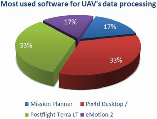
ENVI software has been used by Al-Amin Hoque et al. (2019); Esmail et al. (Mohammed et al., 2019); Nassar et al. (Karim et al., 2019); Joevivek et al. (Joevivek & Saravanan Sakthivel, 2018); Abu Zed et al. (Zed Abu et al., 2018); Duarte et al. (2018); Cenci et al. (Luca et al., 2017); Salghuna & Bharathvaj (Salghuna & Aravind Bharathvaj, 2015); Petropoulos et al. (George et al., 2015); Aiello et al. (Antonello et al., 2015); Gudina et al. (Gudina Feyisa et al., 2014); Sekovski et al. (Ivan et al., 2014); Joevivek et al. (Joevivek & Saravanan Sakthivel, 2013); Addo et al. (2011); Kawakubo et al. (2011); Taha & Elbeih (LGEd & Elbeih, 2010); Wang et al. (Zifeng et al., 2018). Agisoft PhotoScan has been used by Gonçalves et al. (Gil et al., 2019); Nahon et al. (Alphonse et al., 2019); Horacio et al. (Jesús et al., 2019); Letortu et al. (Pauline et al., 2018); Nikolakopoulos et al. (Nikolakopoulos Konstantinos & George, 2017); Papakonstantinou et al. (2016); Casella et al. (2016); Chikhradze et al. (Nino et al., 2015); and Elsner et al. (Elsner Paul et al., 2015). QGIS has been used by Chikhradze et al. (Nino et al., 2015). MapInfo has been used by Fromard et al. (2004). IDRISI Selva has been used by Geosci et al. (Arab et al., 2015); Shalaby and Tateishi (Adel & Ryutaro, 2007). GIS MGE has been used by Chen et al. (Shui-sen Chen et al., 2005). SAGA-GIS has been used by Nahon, et al. (Alphonse et al., 2019). Microsoft Excel has been used by Sandeep et al. (2018) and Thampanya et al. (Thampanya et al., 2006). SPSS has been used by Cui & Li (Bu-Li & Xiao-Yan, 2011) and Thampanya et al. Thampanya et al. (2006). AUTOCAD has been used by In-Ho et al. (Kim et al., 2013) and Sesli et al. (Faik et al., 2008). PG-STTEMER v.4.2. has been used by Kim et al. (2013). Adobe Photoshop Lightroom has been used by Marcaccio et al. (James et al., 2015). SNAP (Sentinel Application Platform) has been used by Konko et al. (Yawo et al., 2018). WXTide32 has been used by Majed et al. (Bouchahma et al., 2012). SHOREX tool has been used by Cabezas-Rabadán et al. (Cabezas-Rabadán et al., 2019). PCI Geomalties Inc has been used by Fletcher et al. (2003). DORIS has been used by Vandebroek et al. (2017). SPINUA has been used by Bruno et al. (Francesca et al., 2016). GEOBIA has been used by Papakonstantinou et al. (Papakonstantinou et al., 2016). MATLAB has been used by Valentini et al. (2017); Turner et al. (2016) and Aiello et al. (2015). The software for UAV’s were categorized separately as they are a modern research tools. So, Mission Planner has been used by (Papakonstantinou et al., 2016). Pix4d has been used by Nikolakopoulos et al. (Nikolakopoulos Konstantinos & George, 2017). Postflight Terra LT and eMotion-2 have been used by Chikhradze et al. (2015).

Erosion/accretion methods and algorithms

Many researchers have dealt with the use of various models and algorithms to calculate erosion/accretion numerically and in addition comparing results tried to estimate the future coastal behavior. RUSLE model has been used by Ganasri and Ramesh (2016), while RUSLE and UPSED models have been used by Aiello et al. (Antonello et al., 2015). Volumetric Changes in beaches’ sand studied by Horacio et al. (Jesús et al., 2019); Kaliraj et al. (2017); Sakthivel et al. (2014); Gares et al. (Gares Paul et al., 2006). CVI (coastal vulnerability index) is another significant feature that researchers used (Hoque et al., 2019; Jana & Bhattacharya, 2013; Joevivek & Saravanan Sakthivel, 2013; Mujabar & Chandrasekar, 2013; Nageswara Rao et al., 2008; Ratna et al., 2018). Tracer stick method has been used by Schwarzer et al. (2003). Beach width (BW) has been used by Cabezas-Rabadán et al. (2019) while AEHR (Annual Erosion Hazard Rate) has been used by Fletcher et al. (Charles et al., 2003).

Methods

Meta-analysis

We gathered hundreds of published articles that reported methods of shoreline monitoring and proposed indices and methodologies. This broad spectrum of studies included a variety of data such as aerial photos, different sensor types, GPS and topo-sheets, satellite, UAV’s and radar images. For each article, we registered the high spot of the study and the index that being used for monitoring the shoreline position determination. Finally, all the collected features were sorted and classified in a Microsoft Excel Sheet and statistical charts were created to make it easier to draw relevant conclusions (figure 2).

Furthermore, this meta-analysis targets to highlight both, some shortcomings in the literature and the good practices that have mainly been used regarding the subject.

Figure 2. Flow chart of methodology used to get to meta-analysis review paper

Year of publication

More than seventy percent (70%) of the studies were published during 2013–2019 (figure 3). This can be directly combined with the fact that researchers over the last decade had the ability to use instruments and data for their studies with improved accuracy (i.e. GNSS techniques, GPS and satellites with 0.01 m and 0.5 m spatial resolution, respectively). Furthermore, from figure 3 we can realize that there has been a strong upward trend in the study of the phenomenon of coastal erosion in the last 20 years (blue line), a fact that proves the existence of the problem and reveals the real concern of the scientific community.

Figure 3. Studies published between 2000 and 2019 being referenced in current paper. Blue line represents the total number of studies

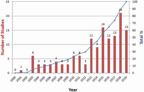
Figure 4. Rates of studies that have been funded

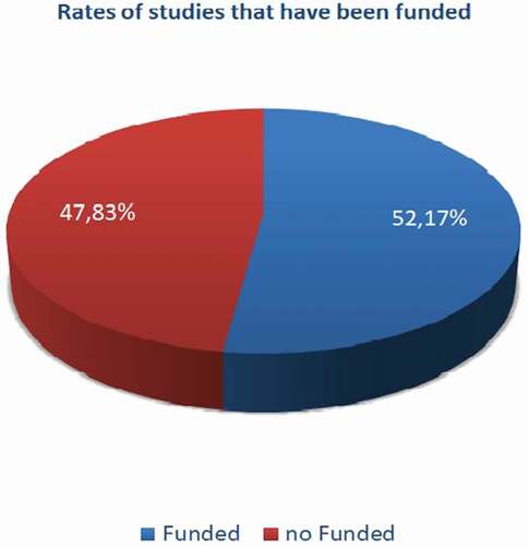
At the same time, in figure 4 we can see that the growth trend in the number of studies in the last two decades can be combined with the concern of the governments and several institutes which have funded the relevant studies. The rate 47.83% of “no funded” is a critical point which being occurred during this study and indicates that one in two studies of coastal erosion issue is being proceeded by researchers without financial support and this should be changed in the next years in order to improve the quality of the results as well as free of charge low-resolution data were used frequently and so the results based on them are limited.

Periods of interest

We distinguished four categories of periods (n in years) which researches work on; a) n ≤ 10, b) 10 < n ≤ 30, c) 30 < n ≤ 70 and d) n > 70 and we found an equal distribution between the first three classes as figure 5 shows.

Figure 5. Four categories of periods (n in years) which researches work on; a) n ≤ 10, b) 10 < n ≤ 30, c) 30 < n ≤ 70, d) n > 70

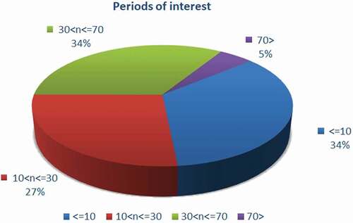
From the diagram above it is obvious that researches are concerned equally for the 10 or less years (a & c period interval). Particularly for the (a) period we can assume that that is happed probably due to the fact that new and accurate data of these years are available as mentioned before. Moreover, the (c) period (30 < n ≤ 70) seems to be in great interest probably due to the fact that many researchers have tried to combine many types of available data due to the time. Furthermore, the (b) period (10 < n ≤ 30) is in great demand as it represents a sort-term period which is most peoples’ concern.

Finally, the (d) period should include historical data, i.e. old maps and aerial photos which are in low accuracy and their scope is most for the study of the diachronic evolution of an area.

Materials

Through literature we found and recorded many types of data that were used in researches such as Topo-sheets, aerial photos, satellite, RADAR and UAV’s images (figure 6).

Figure 6. The most common data sources used in shoreline monitoring

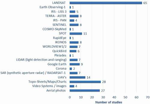
As we can observe from figure 6 the majority of the researchers used mainly three data sets, Landsat satellite, aerial photos and topo-sheets. The specific data sets present two main advantages: Low cost or no cost at all and extensive historical archives that refers for many decades in the past. Moreover, Landsat series (MSS, TM, ETM+, OLI) were the unique continuous mission for nearly 50 years. The rise in the use of UAV imagery is noticeable and proves that researchers have found in UAV’s a low cost but also accurate survey method. Moreover, high-resolution satellite images such as Worldview1/2, QuickBird and Pleiades are not in great demand per study because of their high cost of acquisition and the small extend per scene.

On the other hand, if we sum up all the types of satellites (table 5) and classify them into three types a) High resolution, b) Medium resolution and c) Low resolution, we could note that the above conclusion is overturned (figure 7). As it can be observed in figure 7 in 62 studies high – resolution data was used while low – resolution data was used in 71 studies. This difference of nine studies represents only a 5.5% difference between the high – and low – resolution data in total. This small difference in frequency of use between the freely available low-resolution data such as Landsat and the high-cost data like Worldview could be explained if we took into consideration that always there is a need for validation of the results. Thus, many researchers execute their studies using free of charge low and medium-resolution satellite images. However, the same researchers prefer to use high–resolution images which are more accurate for the verification of the results.

Figure 7. Classification of data in three categories according to spatial resolution

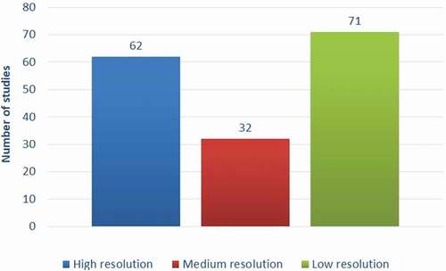
Table 5. Data sources classified by spatial resolution a) High resolution, b) Medium resolution and c) Low resolution

High resolution (< 5 m)	UAV’s
	SAR (synthetic aperture radar)/RADARSAT-1
	Corona
	Google Earth
	LiDAR (light detection and ranging)
	Pleiades
	QuickBird
	WORLDVIEW1/2
	IKONOS
	RapidEye
Medium resolution (5–20 m)	SPOT (1/2/3/4)
	COSMO-SkyMed
	SENTINEL 2
	TERRA – ASTER
	IRS – PAN
Low resolution (>20 m)	IRS – LISS
	Earth Observing-1
	LANDSAT series

Software statistical analysis

The meta-analysis of the studies also examined the software that were used for the shoreline evolution (figure 8). It is proved that in most of the studies there was not only one software used for the analysis but a combination of them. As it can be observed in figure 8, ArcMap software and its tools (in different versions) has a dominant part in coastal researches (40%). Furthermore, it is assumed that the specific software is widely used mainly thanks to the add-on software (DSAS) which many researchers used to estimate various statistical rates of shoreline movement.

Figure 8. Most common software used in shoreline analysis

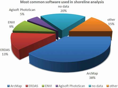
At the same time, ERDAS Imagine, ENVI and Agisoft Photoscan follow the researcher’s preferences. Furthermore, in figure 8 there are two fields which are noticeable, “no data” and “other”. The “no data” field includes studies where no type or name of a software exists but only the expression “GIS software” and the “other” field which includes a variety of software which appeared one, two or three times in the texts being studied (figure 9). Finally, we have chosen to categorize the software for UAV’s data processing separately (figure 10) as they are modern research tools that continuously being developed and moreover they appeared from 2015 onwards in papers that were studied. It is expected in the years to follow that this type of software will be multiplied and improved.

Figure 9. Software with low-frequency appearance in shoreline studies

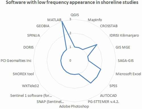
Figure 10. Most used software for UAV’s data processing

Indices

As has been mentioned in paragraph 2.1.4 of the current paper, Boak and Turner (Elizabeth & Ian, 2005) listed 45 various shorelines indices that have been used worldwide in coastal monitoring studies while a summary of shoreline indicators was recently represented by Seynabou Toure et al. (2019). Some of these indicators which have been used from the researchers in order to delineate land from water are presented in figure 11.

Figure 11. Most common indices for delineation of land/water used among studies. Average High-Water Line (AHWL), Automatic Water Extraction Index (AWEI), Normalized Difference Vegetation Index (NDVI), Normalized Difference Water Index (NDWI), Modified Normalized Difference Water Index (MNDWI), High Water Line (HWL), Land Surface Water Index (LSWI), High Tide Line (HTL), Seaward Dune Vegetation Line (SwDVL), Instantaneous Water Line (IWL), Stable Dune Vegetation Line (StDVL), Low Water Level (LWL), Mean Low Water (MLW)

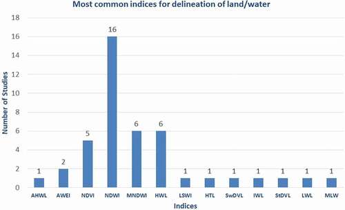
It is obvious that the NDWI index was the most popular among researchers at a rate of 37.21% while the NDVI, MNDWI and HWL rates ranging between 11.63% and 13.95%. It should be noticed that independently from the fact that some indices seems to be more favorable between the researchers, every index has advantages and drawbacks and moreover the final choice is depended on many factors (i.e. available data, equipment, etc.). It is characteristic that the AWEI index has been used only in two studies as we can notice in figure 11. Nevertheless, as has been referred by (Gudina Feyisa et al., 2014) although there are not many studies about the usage of this index, it is very accurate especially when applied in areas where under deep shadow caused by the terrain.

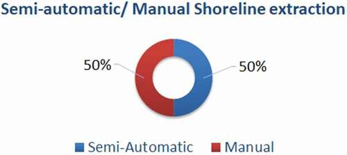
Shoreline extraction methods

In order to delineate the water body from the land surface, except of the traditional manual shoreline extraction which includes field surveys and on-screen digitizing, researchers have tried some automatic classification methods. Such algorithms and equations are presented in figures 12 and 13. It is quite obvious that there is a lot of procedures available for the separation between land and water. These procedures have been called semi-automatic as fully automatic does not exist since now. Furthermore, semi-automatic and manual methods were compared (figure 14) and seems to be equally distributed in the published studies.

Figure 12. Methods used to determine the shoreline

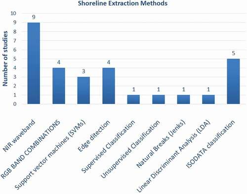
Figure 13. Algorithms and equations used by researchers to delineate the shoreline position

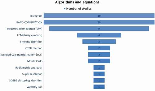
Figure 14. Semi-automatic and manual methods

Digital shoreline analysis system (DSAS) rates

The DSAS is a plug-in to the ArcMap software developed by the United States Geological Survey (USGS) and it is being used for calculating the shoreline change rates. Figure 15 presents the usage of different DSAS rates from the researchers in the studied literature.

Figure 15. Most common indices of DSAS tool; End Point Rate (EPR), Net Shoreline Movement (NSM), Linear Regression Rate (LRR), Shoreline Change Envelope (SCE), Standard Error of Linear Regression (LSE), Confidence Interval of Linear Regression (LCI), R-squared of Linear Regression (LR2), and Weighted Linear Regression (WLR)

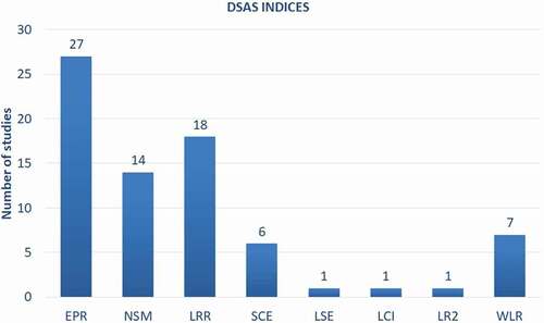
The EPR (End Point Rate), LRR (Linear Regression Rate) and NSM (Net Shoreline Movement) seems to be the most popular with a rate of 36%, 24% and 18,67%, respectively. The net shoreline movement (NSM) calculates the total distance between the newest and the oldest shorelines. The EPR is the NSM rate divided by the time elapsed and the LRR determines a rate-of-change statistic by fitting a least square regression to all shorelines at a specific transect (Himmelstoss et al., 2018).

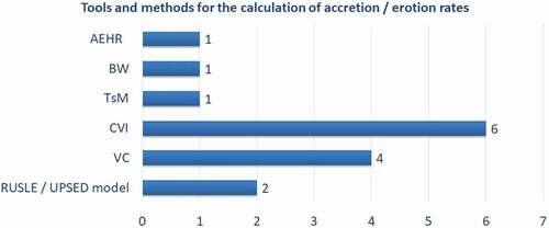
Erosion/accretion methods and algorithms

The final and most interesting part of our research were the tools that have been developed up to now in order to compute the erosion or accretion rate (figure 16). We found that among the tools being used to compute the erosion or accretion rate, coastal vulnerability index (CVI) and volumetric technics of the amount of the sand being lost are the most common tools among researches and being appeared at a rate of 40% and 26,67%, respectively. These methods require the acquisition of several type of data such as topo-sheets, aerial or remote sensing images, ground control points, etc., and thus it is very complex procedure.

Figure 16. Tool and methods for the calculation of accretion/erosion rates; Annual Erosion Hazard Rate (AEHR), Beach Width (BW), Tracer stick method (TsM), Coastal Vulnerability Index (CVI), Volumetric Changes (VC), Revised Universal Soil Loss Equation (RUSLE), Unit Stream Power – based Erosion Deposition (UPSED)

Citations

A list of the most referenced publications by articles referred in coastal erosion/accretion field using remote sensing is presented in table 6. The article that received the highest number of citations was “Management of Coastal Erosion Using Remote Sensing and GIS Techniques”, with a total of 471 citations in Scopus published in the International Journal of Ocean and Climate Systems in 2014.

Table 6. Top 10 cited articles in Scopus in the present study literature

	Researchers	Title	Number of citations
	Saravanan, Sakthivel et al., 2014	Management of Coastal Erosion Using Remote Sensing and GIS Techniques	471
	Paul M. Cooley, David G. Barber, 2003	Remote Sensing of the Coastal Zone of Tropical Lakes Using Synthetic Aperture Radar and Optical Data	471
	Mujabar, P.S. et.al.,2013	Shoreline change analysis along the coast between Kanyakumari and Tuticorin of India using remote sensing and GIS	457
	Raju Aedla, 2015	Automatic Shoreline Detection and Change Detection Analysis of Netravati-GurpurRivermouth Using Histogram Equalization and Adaptive Thresholding Techniques	159
	Cabezas-Rabadán, Carlos et.al.,2019	Characterizing beach changes using high-frequency Sentinel-2 derived shorelines on the Valencian coast (Spanish Mediterranean)	151
	M.A. Davidson et al., 2010	Forecasting seasonal to multi-year shoreline change	150
	Bera, Rakesh & Maiti, Ramkrishna, 2019	Quantitative analysis of erosion and accretion (1975–2017) using DSAS-A study on Indian Sundarbans	146
	Bu-Li Cui, Xiao-Yan Li, 2011	Coastline change of the Yellow River estuary and its response to the sediment and runoff (1976–2005)	143
	Salim, Fatima et al., 2018	Application of a Geomatics Approach for the Diachronic Study of the Meditterannean Coastline Case of Tangier Bay	134
	Robertson, William et.al.,2004	Mapping Shoreline Position Using Airborne Laser Altimetry	129

Conclusions

One hundred thirty-eight studies from the literature reporting remote sensing data, GIS methods, materials and indices used worldwide to estimate the shoreline evolution, have been analyzed. Our aim was to define the usage of such techniques and methods and finally through the meta-analysis to highlight the most dominant indicators, software and methods followed by researchers the last 20-years relative to the coastal erosion/accretion subject. Furthermore this review targets to emerged some critical points through studied literature such as a) the low rate of high-resolution satellite images usage in a subject where the accuracy is prerequisite b) the necessity of the Landsat images being improved as they are the only ones related to the distant past and freely available, c) the usage of the new generation of UAV’s since 2015 as an alternative low-cost source for very high accurate imagery d) the fact that 50% of the studies for coastal erosion is being proceeded without financial support and thus the scientists are obliged to use only freely available data.

Applying the methodology of meta-analysis we have found that there has been a strong upward trend in the study of the phenomenon of coastal erosion in the last twenty years and there are three interesting periods which seems to be equally distributed at a rate of 35%: a) below the 10 years, b) 10 to 30 years and c) 30 to 70 years, while for a period of more than 70 years there seems to be little interest since it is quite difficult to retrieve the necessary historical data. Furthermore, the usage of Landsat satellite images dominates among researchers at a rate of up to 40% while high-resolution data such as IKONOS, Worldview1-2, QuickBird, Pleiades, etc., data seems to lag far behind at less than 5%. This high range is as Landsat images are freely available and very useful to diachronic studies. The usage of medium spatial resolution data such as SPOT (1/2/3/4) and Sentinel ranges from 5% to 7% in general. The UAV imagery is noticeable at a rate of 8% and seems that it will be used widely in the future as it is adopted by the researchers from 2015 onwards. Regarding the favorite software in the studies, ArcMap is being used at a rate of 38% of them, while a sum of the studies that have used software without reference to its type or name and software that has been used occasionally one to three times are at a rate of 35%. ArcMap software has those great rates mainly because of the DSAS add-on tool which is very common among researchers. Moreover, the NWDI indicator has been used by most of researchers to delineate land from water at a rate of 37,21%. In addition, we classified the shoreline extraction methods in two main categories a) semi-automatic and b) manual which are equally distributed. Finally, among the tools being used to compute the erosion or accretion rate, coastal vulnerability index (CVI) and volumetric techniques of the amount of the sand being lost are the most common tools among researches and being appeared at a rate of 40% and 26,67%, respectively.

This study is not intended to criticize neither the methods nor the results being mentioned but to give the opportunity to the researchers (especially the new ones) to have an overall view of the subject for the last 20 years with just a glimpse. It should be clear that the results as represented in the previous pages refer just to the most famous values among the others in the papers being studied and do not propose the best of them because every index has its advantages and drawbacks and moreover the final choice is depended on many factors. We believe that the results represent the researcher’s favorable trend of the materials and methods about the same issue: the coastal erosion and the shoreline evolution.

Disclosure statement

The authors declare no conflict of interest.

Additional information

Funding

This research did not receive any specific grant from funding agencies in the public, commercial, or not-for-profit sectors.

References

- Ablain, M., Becker, M., Benveniste, J., Cazenave, A., Champollion, N., Ciccarelli, S., Jevrejeva, S., Cozannet, G. L., Nicoletta, L., Loisel, H., Long, N., Maisongrande, P., Mallet, C., Marta, M., Menéndez, M., Meyssignac, B., Plater, A. J., Raucoules, D., Andrea, T., Vignudelli, S., … Wöppelmann, G. (2016). White paper: Monitoring the evolution of coastal zones under various forcing factors using space-based observing systems. Geography, Environmental Science.
- Addo, K. A. (2009). Detection of Coastal Erosion Hotspots in Accra, Ghana. Journal of Sustainable Development in Africa, 11. https://www.researchgate.net/publication/202184117_Detection_of_Coastal_Erosion_Hotspots_in_Accra_Ghana
- Addo, K. A., Quashigah, K. S., & Kufogbe, K. S. (2011). Quantitative analysis of shoreline change using medium resolution satellite imagery in Keta, Ghana. Mar Sci, 1(1), 1–9. https://doi.org/https://doi.org/10.5923/j.ms.20110101.01
- Adel, S., & Ryutaro, T. (2007). Remote sensing and GIS for mapping and monitoring land cover and land-use changes in the Northwestern coastal zone of Egypt. Applied Geography, 27(1), 28–41. https://doi.org/https://doi.org/10.1016/j.apgeog.2006.09.004
- Alesheikh, A. A., Ghorbanali, A., & Talebzadeh, A. (2004) Generation the coastline change map for Urmia Lake by TM and ETM+ imagery. Map Asia Conference, Beijing, China.
- Alessandro, B., Schiavon, G., & Solimini, D. (2008). Fusion of high resolution polarimetric SAR and multi-spectral optical data for precision viticulure.IGARSS 2008 - 2008 IEEE International Geoscience and Remote Sensing Symposium,3, 1000. Boston, MA, USA. https://doi.org/https://doi.org/10.1109/IGARSS.2008.4779521
- Alexandrakis, G., Manasakis, C., & Kampanis, N. A. (2015). Valuating the effects of beach erosion to tourism revenue A management perspective. Ocean Coast. Manag, 111, 1–11. https://doi.org/https://doi.org/10.1016/j.ocecoaman.2015.04.001
- Alfredo, G., Amaro, V., Helenice, V., & Marco, D. (2005). A method for coastline evolution analysis using GIS and remote sensing - A case study from the Guamaré City, northeast Brazil. J Coast Res,21, 412–421. https://www.researchgate.net/publication/290671061_A_method_for_coastline_evolution_analysis_using_GIS_and_remote_sensing_-_A_case_study_from_the_Guamare_City_northeast_Brazil
- Aliakbar, R., Rezvan, N., & Mehdi, R. (2010). Monitoring of caspian sea coastline changes using object-oriented techniques. Procedia Environmental Sciences, 2, 416–426. https://doi.org/https://doi.org/10.1016/j.proenv.2010.10.046
- Alphonse, N., Pere, M., Marta, B., Jennifer, S., Sylvain, C., & Cédrik, F. (2019). Corridor mapping of sandy coastal foredunes with UAS photogrammetry and mobile laser scanning. Remote Sensing, 11(11), 1352. https://doi.org/https://doi.org/10.3390/rs11111352
- Anand, R., Chandrasekar, N., Kaliraj, S., & Magesh, N. S. (2016). Shoreline change rate and erosion risk assessment along the Trou Aux Biches – Mont Choisy beach on the northwest coast of Mauritius using GIS-DSAS technique. Environmental Earth Sciences, 75(5), 1–12. https://doi.org/https://doi.org/10.1007/s12665-016-5311-4
- Andredaki, M., Georgoulas, A., Hrissanthou, V., & Kotsovinos, N. (2014). Assessment of reservoir sedimentation effect on coastal erosion in the case of Nestos River, Greece. International Journal of Sediment Research, 29(1), 34–48. Volume. https://doi.org/https://doi.org/10.1016/S1001-6279(14)60020-2
- Annibale Guariglia, A., Buonamassa, A., Angela, L., Rocco, S., Maria, T., Angelo, Z., & Antonio, C. (2009). A multisource approach for coastline mapping and identification of shoreline changes. Annals of Geophysics, 49. https://doi.org/https://doi.org/10.4401/ag-3155
- Antonello, A., Filomena, C., Guido, P., & Giuseppe, S. (2013). Shoreline variations and coastal dynamics: A space-time data analysis of the Jonian littoral, Italy. Estuarine, Coastal and Shelf Science, 129, 124–135. https://doi.org/https://doi.org/10.1016/j.ecss.2013.06.012
- Antonello, A., Maria, A., & Filomena, C. (2015). Remote sensing and GIS to assess soil erosion with RUSLE3D and USPED at river basin scale in southern Italy. CATENA, 131, 174–185. https://doi.org/https://doi.org/10.1016/j.catena.2015.04.003
- Aris, M. M., Hussein, A., Dey, S., Susanto, B., & Lorenz, K. (2008). Coastal dynamic and shoreline mapping: Multi-sources spatial data analysis in Semarang Indonesia. Environmental Monitoring and Assessment, 142(1–3), 297–308. https://doi.org/https://doi.org/10.1007/s10661-007-9929-2
- Asib, A., Frances, D., Rizwan, N., & Clare, W. (2018). Where is the coast? Monitoring coastal land dynamics in Bangladesh: An integrated management approach using GIS and remote sensing techniques. Ocean & Coastal Management, 151, 10–24. https://doi.org/https://doi.org/10.1016/j.ocecoaman.2017.10.030
- Ayadi, K., Boutiba, M., Sabatier, F., & Guettouche, M. S. (2016). Detection and analysis of historical variations in the shoreline, using digital aerial photos, satellite images, and topographic surveys DGPS: Case of the Bejaia bay (East Algeria). Arabian Journal of Geosciences, 9(1), 26. https://doi.org/https://doi.org/10.1007/s12517-015-2043-9
- Bakhoum, P. W., Ndour, A., Niang, I., Sambou, B., Traore, V. B., Diaw, A. T., Sambou, H., & Ndiaye, M. L. (2017). Coastline mobility of Goree Island (Senegal) from 1942 to 2011. Marine Science, 7(1), 1–9. https://doi.org/https://doi.org/10.5923/j.ms.20170701.01
- Behling, B. R., Milewski, M. R., & Chabrillat, C. S. (2018). Spatiotemporal shoreline dynamics of Namibian coastal lagoons derived by a dense remote sensing time series approach. International Journal of Applied Earth Observation and Geoinformation, 68, 262–271. https://doi.org/https://doi.org/10.1016/j.jag.2018.01.009
- Bera, R., & Maiti, R. (2019). Quantitative analysis of erosion and accretion (1975-2017) using DSAS — A study on Indian Sundarbans. Regional Studies in Marine Science, 28, 100583. https://doi.org/https://doi.org/10.1016/j.rsma.2019.100583
- Bird, E. (2008). Coastal geomorphology: An introduction (2nd ed ed.). Wiley.
- Bouchahma, M., Yan, W., Wanglin, M., & Mohamed, O. (2012). Island coastline change detection based on image processing and remote sensing. Computer and Information Science, 5(3), 27–36. https://doi.org/https://doi.org/10.5539/cis.v5n3p27
- Brock, J., Sallenger, A., Krabill, W. B., Swift, R., & Wright, C. (2001). Recognition of fiducial surfaces in lidar surveys of coastal topography. Photogrammetric Engineering and Remote Sensing, 67(11), 1245–1258. https://www.researchgate.net/publication/287562794_Recognition_of_Fiducial_Surfaces_in_Lidar_Surveys_of_Coastal_Topography
- Bulent, B. B., Huseyin Bayraktar, H., Helvaci, C., & Ugur, A. (2004). Coastline change detection using Corona, Spot and IRS 1d images. https://www.researchgate.net/publication/237414716_Coast_line_change_detection_using_Corona_Spot_and_IRS_1d_images
- Bu-Li, C., & Xiao-Yan, L. (2011). Coastline change of the Yellow River estuary and its response to the sediment and runoff (1976–2005). Geomorphology, 127(1–2), 32–40. https://doi.org/https://doi.org/10.1016/j.geomorph.2010.12.001
- Burningham, B. H., & French, F. J. (2017). Understanding coastal change using shoreline trend analysis supported by cluster-based segmentation. Geomorphology, 282, 131–149. https://doi.org/https://doi.org/10.1016/j.geomorph.2016.12.029
- Cabezas-Rabadán, C., Pardo-Pascual, J. E., Palomar-Vázquez, J., & Fernández-Sarría, A. (2019). Characterizing beach changes using high-frequency Sentinel-2 derived shorelines on the Valencian coast (Spanish Mediterranean). Science of the Total Environment, 691, 216–231. https://doi.org/https://doi.org/10.1016/j.scitotenv.2019.07.084
- Carolina, M., Manuel, C.-L., Patricio, W., Héctor, H., Eduardo, G., & Roberto, A. (2018). Coastal erosion in central Chile: A new hazard?. Ocean & Coastal Management, 156, 141–155. https://doi.org/https://doi.org/10.1016/j.ocecoaman.2017.07.011
- Casella, E., Rovere, A., Pedroncini, A., Stark, C. P., Casella, M., Ferrari, M., & Firpo, M. (2016). Drones as tools for monitoring beach topography changes in the Ligurian Sea (NW Mediterranean). Geo-Mar. Lett, 36(2), 151–163. https://doi.org/https://doi.org/10.1007/s00367-016-0435-9
- Chand, P., & Acharya, P. (2010). Shoreline change and sea level rise along coast of Bhitarkanika wildlife sanctuary, Orissa: An analytical approach of remote sensing and statistical techniques. International Journal of Geomatics and Geosciences, 28(1), 436–455. https://www.researchgate.net/publication/301772465
- Charles, F., Rooney, J., Matthew, B., Lim, S. C., & Bruce, R. (2003). Mapping shoreline change using digital orthophotogrammetry on Maui, Hawaii. Journal of Coastal Research, 38,106–124. https://www.jstor.org/stable/25736602
- Chen, B., Benqing, Y., Yanming, Y., Wen, H., Hongtao, H., Hailin, R., Zaiming Zhou, Z., Kai Luo, K., & Fuhuang Zhong, F. (2018). High-resolution monitoring of beach topography and its change using unmanned aerial vehicle imagery. Ocean & Coastal Management, 160, 103–116. https://doi.org/https://doi.org/10.1016/j.ocecoaman.2018.04.007
- Chen, C. C., Jiaoqi, F., Shuai, Z., & Xin, Z. (2019). Coastline information extraction based on the tasseled cap transformation of Landsat-8 OLI images. Estuarine, Coastal and Shelf Science, 217, 281–291. https://doi.org/https://doi.org/10.1016/j.ecss.2018.10.021
- Chen, S.-S., Chen, L.-F., Liu, Q.-H., Xia, L., & Tan, Q. (2005). Remote sensing and GIS-based integrated analysis of coastal changes and their environmental impacts in Lingding Bay, Pearl River Estuary, South China. Ocean & Coastal Management, 48(1), 65–83. https://doi.org/https://doi.org/10.1016/j.ocecoaman.2004.11.004
- Chen, -W.-W., & Chang, H.-K. (2009). Estimation of shoreline position and change from satellite images considering tidal variation. Estuarine Coastal and SHELF Science - ESTUAR COAST SHELF SCI, 84(1), 54–60. https://doi.org/https://doi.org/10.1016/j.ecss.2009.06.002
- Christopher, D., Mitchell, H., Ian, T., Matheen, A., Nashwan, A., & Will, G. (2015). UAV applications to coastal engineering. Auckland, New Zealand. https://www.researchgate.net/publication/282606382_UAV_Applications_to_Coastal_Engineering
- Coastal Engineering Research Center (CERC). (1984). Shore protection manual. US Army Corps of Engineers, Washington DC, I, 597. II, 603. https://www.scirp.org/(S(vtj3fa45qm1ean45vvffcz55))/reference/ReferencesPapers.aspx?ReferenceID=1527818
- Cooley Paul, M., & Barber David, G. (2003). Remote sensing of the coastal zone of tropical lakes using synthetic aperture radar and optical data. Journal of Great Lakes Research, 29(2), 62–75. https://doi.org/https://doi.org/10.1016/S0380-1330(03)70539-5
- Cracknell Arthur, P. (2018). The development of remote sensing in the last 40 years. International Journal of Remote Sensing, 39(23), 8387–8427. https://doi.org/https://doi.org/10.1080/01431161.2018.1550919
- Da Guia Albuquerque, M., Espinoza, J., Teixeira, P., Oliveira, A., Correa, I., & Calliari, L. (2013). Erosion or coastal variability: An evaluation of the DSAS and the change polygon methods for the determination of erosive processes on sandy beaches. Journal of Coastal Research, 65(sp2), 1710–1714. https://doi.org/https://doi.org/10.2112/SI65-289.1
- Davidson, M. A., Lewis, R. P., & Turner, I. L. (2010). Forecasting seasonal to multi-year shoreline change. Coastal Engineering, 57(6), 620–629. https://doi.org/https://doi.org/10.1016/j.coastaleng.2010.02.001
- Davidson Mark, A., Turner Ian, L., Kristen Splinter, D., & Harley Mitchel, D. (2017). Annual prediction of shoreline erosion and subsequent recovery. Coastal Engineering, 130, 14–25. https://doi.org/https://doi.org/10.1016/j.coastaleng.2017.09.008
- Del Río, L., Javier, G. F., & Benavente, J. (2013). Shoreline change patterns in sandy coasts. A Case Study in SW Spain, Geomorphology, 196, 252–266. https://doi.org/https://doi.org/10.1016/j.geomorph.2012.07.027
- Di, K., Wang, J., Ma, R., & Li, R. (2003) Automatic shoreline extraction from high-resolution Ikonos satellite imagery. In Proceeding of the Annual ASPRS Conference, Anchorage, Alaska.
- Do, A. T., De Vries, S., & Stive, M. J. (2018). The estimation and evaluation of shoreline locations, shoreline-change rates, and coastal volume changes derived from Landsat images. J. Coast. Res, 35(1), 56–71. https://www.researchgate.net/publication/329913044_The_Estimation_and_Evaluation_of_Shoreline_Locations_Shoreline-Change_Rates_and_Coastal_Volume_Changes_Derived_from_Landsat_Images
- Dolan, R., Hayden, B. P., May, P., & May, S. (1980). The reliability of shoreline change measurements from aerial photographs. Shore and Beach, 48, 22–29. https://www.scopus.com/record/display.uri?eid=2-s2.0-0019068233&origin=inward&txGid=62a249f9ca7c146f6a3631d12138fde9
- Duarte, C. R., De Miranda, F. P., Landau, L., Souto, M. V. S., Sabadia, J. A. B., Claudio Ângelo Da Silva, N., Linara Ivina De Castro, R., & Damasceno, A. M. (2018). Short-time analysis of shoreline based on RapidEye satellite images in the terminal area of Pecém Port, Ceará, Brazil. International Journal of Remote Sensing, 39(13), 4376–4389. https://doi.org/https://doi.org/10.1080/01431161.2018.1457229
- El-Asmar, H. M., & Hereher, M. E. (2011). Change detection of the coastal zone east of the Nile Delta using remote sensing. Environ Earth Sci, 62(4), 769. https://doi.org/https://doi.org/10.1007/s12665-010-0564-9
- Elizabeth, B. H., & Ian, T. L. (2005). Shoreline Definition and Detection: A Review. Journal of Coastal Research, 2005 (214), 688–703. 1 July 2005. https://doi.org/https://doi.org/10.2112/03-0071.1.
- Faik, S., Fevzi, K., Ismail, C., & Nihat, A. (2008). Monitoring the changing position of coastlines using aerial and satellite image data: An example from the eastern coast of Trabzon, Turkey. Environmental Monitoring and Assessment, 153(1–4), 391–403. https://doi.org/https://doi.org/10.1007/s10661-008-0366-7
- Fatima, S., Mohammed, H., Lech-Hab, H., Ahmed, R., & Abdelkrim, A. (2018). Application of a geomatics approach for the diachronic study of the Mediterranean coastline case of Tangier Bay. International Journal of Geosciences, 09(6), 320–336. https://doi.org/https://doi.org/10.4236/ijg.2018.96020
- Fenster, M. S., & Dolan, R. (1999). Mapping erosion hazard areas in the city of Virginia Beach: Journal of Coastal Research. Special Issue, 28, 58–68. https://www.jstor.org/stable/25736186?seq=1
- Ferdinando, N., Andrea, B., Maurizio, M., Guido, B., & Di Luccio, D. (2018) Shoreline erosion of microtidal beaches examined with UAV and remote sensing techniques. IEEE International Workshop on Metrology for the Sea; Learning to Measure Sea Health Parameters (MetroSea), Bari, Italy 162–166. https://doi.org/https://doi.org/10.1109/MetroSea.2018.8657843
- Ford Murray, R., & Kench Paul, S. (2015). Multi-decadal shoreline changes in response to sea level rise in the Marshall Islands. Anthropocene, 11, 14–24. https://doi.org/https://doi.org/10.1016/j.ancene.2015.11.002
- Francesca, B. M., Gianluca, M. M., Michele, M., Raffaele, N., Alberto, M., & Maria, C. (2016). Coastal observation through Cosmo-SkyMed high-resolution SAR images. Journal of Coastal Research. 75 (sp1), Part, 2, 795–799. https://doi.org/https://doi.org/10.2112/SI75-160.1
- Fromard, F., Vega, C., & Proisy, C. (2004). Half a century of dynamic coastal change affecting mangrove shorelines of French Guiana. A Case Study Based on Remote Sensing Data Analyses and Field Surveys, Marine Geology, 208 (2-4).
- Fugara, A., A’Kif, B. L., & Biswajeet, P. (2011). Semi-automated procedures for shoreline extraction using single RADARSAT-1 SAR image. Estuarine, Coastal and Shelf Science Journal, 95(4). https://doi.org/10.1016/j.ecss.2011.10.009
- Ganasri, B. P., & Ramesh, H. (2016). Assessment of soil erosion by RUSLE model using remote sensing and GIS - A case study of Nethravathi Basin. Geoscience Frontiers, 7(6), 953–961. https://doi.org/https://doi.org/10.1016/j.gsf.2015.10.007
- Ganzorig, M., Amarsaikhan, D., Batbayar, G., Bulgan, G., & Munkherdene, A. (2006) The investigation of land surface features using optical and SAR images. Asian Conference on Remote Sensing ACRS http://www.aars-acrs.org/acrs/proceeding/ACRS2006/Papers/I-1_I4.pdf
- Gens, R. (2010). Remote sensing of coastlines: Detection, extraction and monitoring. International Journal of Remote Sensing, 31(7), 1819–1836. https://doi.org/https://doi.org/10.1080/01431160902926673
- George, P. P., Dionissios, K. P., Hywel, G. M., & Paraskevi, D. P. (2015). Remote sensing and GIS analysis for mapping spatio-temporal changes of erosion and deposition of two Mediterranean river deltas: The case of the Axios and Aliakmonas rivers, Greece. International Journal of Applied Earth Observation and Geoinformation, 35(part Β), 217–228. https://doi.org/https://doi.org/10.1016/j.jag.2014.08.004
- Gil, G., Sara, S., Diogo, D., & José, S. (2019). Monitoring Local Shoreline Changes by Integrating UASs, Airborne LiDAR, Historical Images and Orthophotos. Heraklion, Crete, Greece.
- Gudina Feyisa, L., Henrik, M., Rasmus, F., & Proud Simon, R. (2014). Automated water extraction index: A new technique for surface water mapping using Landsat imagery. Remote Sensing of Environment, 140, 23–35. https://doi.org/https://doi.org/10.1016/j.rse.2013.08.029
- Hashmi, G. M. D., & Sajid, A. (2018). GIS-based analysis and modeling of coastline erosion and accretion along the Coast of Sindh Pakistan. Journal of Coastal Zone Management, 21(1).
- Herold, N. D., Haack, B. N., & Solomon, E. (2004). An evaluation of radar texture for land use/cover extraction in varied landscapes. International Journal of Applied and Earth Observation and Geoinformation, 5(2), 113–128.
- Hervé, T., Benoît, D., Nicolas, C., Jacob, K., & Jean-Paul, R. (2005). Monitoring coastal evolution and associated littoral hazards of French Guiana shoreline with radar images. Comptes Rendus Geoscience, 337(13), 1140–1153. https://doi.org/https://doi.org/10.1016/j.crte.2005.05.013
- Himmelstoss, E. A., Henderson, R. E., Kratzmann, M. G., & Farris, A. S. (2018) Digital Shoreline Analysis System (DSAS) version 5.0 user guide: U.S. Geological Survey Open-File Report 2018–1179, 110 p. https://doi.org/https://doi.org/10.3133/ofr20181179
- Hoque, M. A.-A., Ahmed, N., Pradhan, B., & Roy, S. (2019). Assessment of coastal vulnerability to multi-hazardous events using geospatial techniques along the eastern coast of Bangladesh. Ocean & Coastal Management, 181, 104898. https://doi.org/https://doi.org/10.1016/j.ocecoaman.2019.104898
- Ian, T. L., Mitchell, H. D., & Christopher, D. D. (2016). UAVs for coastal surveying. Coastal Engineering, 114, 19–24. https://doi.org/https://doi.org/10.1016/j.coastaleng.2016.03.011
- Ivan, S., Francesco, S., Francesco, M., & Del Rio, L. (2014). Image classification methods applied to shoreline extraction on very high-resolution multispectral imagery. International Journal of Remote Sensing, 35(10), 3556–3578. https://doi.org/https://doi.org/10.1080/01431161.2014.907939
- Jaime, A.-C., Elena, S.-G., Pardo-Pascual Josep, E., Balaguer-Beser Angel, A., & Jesús, P.-V. (2016). Evaluation of annual mean shoreline position deduced from Landsat imagery as a mid-term coastal evolution indicator. Marine Geology, 372, 79–88. https://doi.org/https://doi.org/10.1016/j.margeo.2015.12.015
- James, M., Chantel, M., & Patricia, C.-F. 2015. Unmanned aerial vehicles produce high-resolution, seasonally-relevant imagery for classifying wetland vegetation. ISPRS - International archives of the photogrammetry. Remote Sensing and Spatial Information Sciences, XL-1/W4, 249–256. https://doi.org/https://doi.org/10.5194/isprsarchives-XL-1-W4-249-2015.
- Jana, A., & Bhattacharya, A. K. (2013). Assessment of coastal erosion vulnerability around Midnapur-Balasore Coast, Eastern India using integrated remote sensing and GIS techniques. J Indian Soc Remote Sens, 41(3), 675–686. https://doi.org/https://doi.org/10.1007/s12524-012-0251–2
- Jesús, H., Efrén, M.-N., Alan, T. S., & Augusto, P.-A. (2019). Remote sensing monitoring of a coastal-valley earthflow in northwestern Galicia, Spain. CATENA, 178, 276–287. https://doi.org/https://doi.org/10.1016/j.catena.2019.03.028
- Joevivek, V., & Saravanan Sakthivel, C. N. (2013). Coastal vulnerability and shoreline changes for southern tip of India-remote sensing and GIS approach. Journal of Earth Science and Climatic Change, 4. https://doi.org/https://doi.org/10.4172/2157-7617.1000144
- Joevivek, V., & Saravanan Sakthivel, C. N. (2018). Assessing the shoreline trend changes in Southern tip of India. Journal of Coastal Conservation, 23, 283–292. https://doi.org/https://doi.org/10.1007/s11852-018-0657-2
- John, D. L., & Scott, S. G. (2010). Shoreline and beach volume change between 1967 and 2007 at Raine Island, Great Barrier Reef, Australia. Global and Planetary Change, 72(3), 141–154. https://doi.org/https://doi.org/10.1016/j.gloplacha.2010.01.026
- Kaliraj, S., Chandrasekar, N., & Ramachandran, K. (2017). Mapping of coastal landforms and volumetric change analysis in the south-west coast of Kanyakumari, South India using remote sensing and GIS techniques. The Egyptian Journal of Remote Sensing and Space Science, 20(2), 265–282. https://doi.org/https://doi.org/10.1016/j.ejrs.2016.12.006
- Kankara, R. S., Selvan, S., Selvan, C., Markose Vipin, J., Rajan, B., & Arockiaraj, S. (2015). Estimation of long and short term shoreline changes along Andhra Pradesh Coast using remote sensing and GIS techniques. Procedia Engineering, 116, 855–862. https://doi.org/https://doi.org/10.1016/j.proeng.2015.08.374
- Karim, N., Wael, M. E., Hassan, F., Ali, M., Kazuo, N., & Abdelazim, N. (2019). Shoreline change detection using DSAS technique: Case of North Sinai coast, Egypt. Marine Georesources & Geotechnology, 37(1), 81–95. https://doi.org/https://doi.org/10.1080/1064119X.2018.1448912
- Kawakubo, F. S., Morato, R. G., Nader, R. S., & Luchiari, A. (2011). Mapping changes in coastline geomorphic features using Landsat TM and ETM+ imagery: Examples in southeastern Brazil. International Journal of Remote Sensing, 32(9), 2547–2562. https://doi.org/https://doi.org/10.1080/01431161003698419
- Kim, I.-H., Lee, H.-S., & Song, D. (2013). Time series analysis of shoreline changes in Gonghyunjin and songjiho Beaches, South Korea using aerial photographs and remotely sensed imagery. Journal of Coastal Research, 165(sp2), 1415–1420. https://doi.org/https://doi.org/10.2112/SI65-239.1
- Konstantinos, N., Vassilia, K., & Demetrius, R. (2007). Coastal water mapping using satellite hyperspectral data. Spie Newsroom. https://doi.org/https://doi.org/10.1117/2.1200612.0498
- Kroon, A., Davidson, M. A., Aarninkhof, S. G. J., Archetti, R., Armaroli, C., Gonzalez, M., Medri, S., Osorio, A., Aagaard, T., Holman, R. A., & Spanhoff, R. (2007). Application of remote sensing video systems to coastline management problems. Coastal Engineering, 54(6–7), 493–505. https://doi.org/https://doi.org/10.1016/j.coastaleng.2007.01.004
- Kumaravel, S., Ramkumar, T., Gurunanam, B., Suresh, M., & Dharanirajan, K. (2013). An application of remote sensing and GIS Based Shoreline Change Studies—A Case Study in the Cuddalore District, East Coast of Tamilnadu, South India. International Journal of Innovative Technology and Exploring Engineering (IJITEE), 2(4), 211–215. https://www.ijitee.org/wp-content/uploads/papers/v2i4/D0545032413.pdf
- LGEd, T., & Elbeih, S. F. (2010). Investigation of fusion of SAR and Landsat data for shoreline super resolution mapping: The Northeastern Mediterranean sea Mediterranean Sea coast in Egypt. Appl. Geomat, 2 (4), 177–186. 2010. https://doi.org/https://doi.org/10.1007/s12518-010-0033-x
- Liu, Q., & John, T. (2018) Sub-Pixel Technique for Time Series Analysis of Shoreline Changes Based on Multispectral Satellite Imagery. IntechOpen. https://doi.org/https://doi.org/10.5772/intechopen.81789
- Liu, Q., John, T., & Ian, T. (2017). Automatic super-resolution shoreline change monitoring using Landsat archival data: A case study at Narrabeen-Collaroy Beach, Australia. Journal of Applied Remote Sensing, 11(1), 016036. https://doi.org/https://doi.org/10.1117/1.JRS.11.016036
- Liu, Y., Huang, H., Qiu, Z., & Fan, J. (2013). Detecting coastline change from satellite images based on beach slope estimation in a tidal flat. International Journal of Applied Earth Observation and Geoinformation, 23,165–176. https://doi.org/https://doi.org/10.1016/j.jag.2012.12.005
- Louati, M., Saïdi, H. & Zargouni, F. Shoreline change assessment using remote sensing and GIS techniques: a case study of the Medjerda delta coast, Tunisia. Arab J Geosci 8, 4239–4255 (2015). https://doi.org/https://doi.org/10.1007/s12517-014-1472–1
- Louati, M., Saïdi, H. & Zargouni, F. (2015). Shoreline change assessment using remote sensing and GIS techniques: a case study of the Medjerda delta coast, Tunisia. Arab J Geosci 8, 4239–4255. https://doi.org/https://doi.org/10.1007/s12517-014-1472-1
- Luca, C., Leonardo, D., Sousa, L., Michael, P., & Alves, F. (2013). Geomatics for integrated coastal zone management: Multitemporal shoreline analysis and future regional perspective for the Portuguese Central Region. Journal of Coastal Research. 65(sp2), 1349–1354. https://doi.org/https://doi.org/10.2112/SI65-228.1
- Luca, C., Leonardo, D., Μgpina, P., Eduardo, O., Fátima, A., & Michael, P. (2017). Integrating remote sensing and GIS techniques for monitoring and modeling shoreline evolution to support coastal risk management. GIScience & Remote Sensing, 5(3),1–21. https://doi.org/https://doi.org/10.1080/15481603.2017.1376370
- Maglione, P., Parente, C., & Vallario, A. (2015). High resolution satellite images to reconstruct recent evolution of domitian coastline. American Journal of Applied Sciences, 12(7), 506–515. https://doi.org/https://doi.org/10.3844/ajassp.2015.506.515
- Malarvizhi, K., Kumar, S., & Porchelvan, P. (2016). Use of high resolution Google earth satellite imagery in land use map preparation for urban related applications. Procedia Technology, 24, 1835–1842. https://doi.org/https://doi.org/10.1016/j.protcy.2016.05.231
- Manjulavani, K., Supriya, V. M., Suhrullekha, M., & Harish, B. (2017) Detection of shoreline change using geo-spatial techniques along the coast between Kanyakumari and Tuticorin 2017 IEEE International Conference on Power, Control, Signals and Instrumentation Engineering (ICPCSI), Chennai, 2822–2825. https://doi.org/https://doi.org/10.1109/ICPCSI.2017.8392235
- Marghany, M., & Hashim, M. (2010a). Developing adaptive algorithm for automatic detection of geological linear features using RADARSAT-1 SAR data. International Journal of Physical Sciences, 5(14), 2223–2229. https://www.researchgate.net/publication/235781068_Developing_adaptive_algorithm_for_automatic_detection_of_geological_linear_features_using_RADARSAT-1_SAR_data
- McFeeters, S. K. (1996). The use of normalized difference water index (NDWI) in the delineation of open water features. International Journal of Remote Sensing, 17(7), 1425–1432. https://doi.org/https://doi.org/10.1080/01431169608948714
- Mitra, S., Mitra, D., & Abhisek, S. (2017). Performance testing of selected automated coastline detection techniques applied on multispectral satellite imageries. Earth Sci. Inform, 10(3), 321–330. https://doi.org/https://doi.org/10.1007/s12145-017-0289-3
- Mohammad, M., Gholamreza, A., & Mohammad, S. (2018). Integration of spectral histogram and level set for coastline detection in SAR images. IEEE Transactions on Aerospace and Electronic Systems, 55(2), 810–819. https://doi.org/https://doi.org/10.1109/TAES.2018.2865120
- Mohammed, E., Elham, M. W., & Hassan, F. (2019). Assessment and prediction of shoreline change using multi-temporal satellite images and statistics: Case study of Damietta coast, Egypt. Applied Ocean Research, 82, 274–282.apor.2018.11.009
- Mörner, N., & Klein, P. (2017). Coastal Erosion in Yasawa Islands, Fiji. Natural Science, 9(5), 136–142. https://doi.org/https://doi.org/10.4236/ns.2017.95014
- Mujabar, P. S., & Chandrasekar, N. (2013). Shoreline change analysis along the coast between Kanyakumari and Tuticorin of India using remote sensing and GIS. Arab J Geosci, 6(3), 647–664. https://doi.org/https://doi.org/10.1007/s12517-011-0394-4
- Murray, F. (2013). Shoreline changes interpreted from multi-temporal aerial photographs and high resolution satellite images: Wotje Atoll, Marshall Islands. Remote Sensing of Environment, 135, 130–140. https://doi.org/https://doi.org/10.1016/j.rse.2013.03.027
- Nageswara Rao, K., Subraelu, P., Venkateswara Rao, T., Hema Malini, B., Ratheesh, R., Bhattacharya, S., & Rajawat, A. S. (2008). (2008) Sea-level rise and coastal vulnerability: An assessment of Andhra Pradesh coast, India through remote sensing and GIS. J Coast Conserv Coast Conserv, 12(4), 195–207. https://doi.org/https://doi.org/10.1007/s11852-009-0042-2
- Nan, X. (2018). Detecting coastline change with all available Landsat data over 1986–2015: A case study for the State of Texas, USA. Atmosphere, 9(3), 107. https://doi.org/https://doi.org/10.3390/atmos9030107
- Nico, V., Alessandra, S., Gianluca, M. M., & Damiani, L. (2017). New algorithms for shoreline monitoring from coastal video systems. Earth Science Informatics. https://doi.org/https://doi.org/10.1007/s12145-017-0302-x
- Niedermeier, A., Hoja, D., & Lehner, S. (2005). Topography and morphodynamics in the German Bight using SAR and optical remote sensing data. Ocean Dynamics, 55(2), 100–109. https://doi.org/https://doi.org/10.1007/s10236-005-0114-2
- Nikolakopoulos, K., Kyriou, A., Koukouvelas, I., Zygouri, V., & Apostolopoulos, D. (2019). Combination of aerial, satellite, and UAV photogrammetry for mapping the diachronic coastline evolution: The case of Lefkada Island. ISPRS Int. J. Geo Inf, 8(11), 489. https://doi.org/https://doi.org/10.3390/ijgi8110489
- Nikolakopoulos Konstantinos, G., & George, D. (2017) Estimating the accuracy of vectors derived from open data, Proc. SPIE 10428, Earth Resources and Environmental Remote Sensing/GIS Applications VIII, 104280N. Warsaw, Poland. https://doi.org/https://doi.org/10.1117/12.2278275
- Nikolakopoulos Konstantinos, G., Kozarski, D., & Kogkas, S. (2017) Coastal areas mapping using UAV photogrammetry, Proc. SPIE 10428, Earth Resources and Environmental Remote Sensing/GIS Applications VIII, 104280O. Wasaw, Poland. https://doi.org/https://doi.org/10.1117/12.2278121
- Nino, C., Renato, H., Mikheil, E., Giorgi, K., Zurab, J., Nana, B., & George, L. (2015). Close range photogrammetry in the survey of the coastal area geoecological conditions (on the example of portugal), Earth Sciences. special issue: Modern Problems of Geography and Anthropology, 4 (5–1), 35–40. 2015. https://doi.org/https://doi.org/10.11648/j.earth.s.2015040501.17
- Nordstrom, K. F. (2004). Beaches and Dunes of Developed Coasts. Cambridge University Press. https://doi.org/https://doi.org/10.1017/CBO9780511549519
- Pajak, M. J., & Leatherman, S. (2002). The high water line as shoreline indicator. Journal of Coastal Research, 18(2), 329–337. https://www.researchgate.net/publication/279560697_The_high_water_line_as_shoreline_indicator
- Pantanahiran, W. (2019). Using remote sensing data for calculating the coastal erosion in Southern Τthailand. Int. Arch. Photogramm. Remote Sens. Spatial Inf. Sci, XLII-3/W7, 51–56. https://doi.org/https://doi.org/10.5194/isprs-archives-XLII-3-W7-51-2019
- Papakonstantinou, A., Topouzelis, K., & Pavlogeorgatos, G. (2016). Coastline zones identification and 3D coastal mapping using UAV spatial data. ISPRS Int. J. Geo-Information, 5(6), 75. https://doi.org/https://doi.org/10.3390/ijgi5060075
- Paravolidakis, V., Moirogiorgou, K., Ragia, L., Zervakis, M., & Synolakis, C. (2016). Coastline extraction from aerial images based on edge detection. ISPRS Ann. Photogramm. Remote Sens. Spat. Inf. Sci, 3(8), 153–158. https://doi.org/https://doi.org/10.5194/isprs-annals-III-8-153-2016
- Pardo-Pascual, E. J., Jaime, A.-C., Luis, R. A., & Jesús, P.-V. (2012). Automatic extraction of shorelines from Landsat TM and ETM+ multi-temporal images with subpixel precision. Remote Sensing of Environment, 123, 1–11. https://doi.org/https://doi.org/10.1016/j.rse.2012.02.024
- Paul, E., Horn, D., Dornbusch, U., Thomas, I., & Dan, A. (2015) Monitoring mixed sand and gravel beaches using unmanned aerial systems. Environmental Modelling & Software. https://doi.org/https://doi.org/10.1142/9789814689977_0172
- Paul, G., Yong, W., & Stephen, W. (2006). Using LIDAR to monitor a beach nourishment project at Wrightsville Beach, North Carolina, USA. Journal of COASTAL Research - J COASTAL RES, 225, 1206–1219. https://doi.org/https://doi.org/10.2112/06A-0003.1
- Pauline, L., Marion, J., Philippe, G., Jerome, A., Stephane, C., Olivier, M., Robert, D., Le Dantec, N., & Christophe, D. (2018). Examining high-resolution survey methods for monitoring cliff erosion at an operational scale. GIScience & Remote Sensing, 55(4), 457–476. https://doi.org/https://doi.org/10.1080/15481603.2017.1408931
- Peter, R., & Kaminsky George, G. G. (2003). Linking proxy-based and datum-based shorelines on a high-energy coastline: Implications for shoreline change analyses. Journal of Coastal Research, 38, 57–82. https://www.researchgate.net/publication/279696589_Linking_Proxy-Based_and_Datum-Based_Shorelines_on_a_High-Energy_Coastline_Implications_for_Shoreline_Change_Analyses
- Pradhan, B. (2009). Flood susceptible mapping and risk area estimation using logistic regression. GIS and Remote Sensing. Journal of Spatial Hydrology, 9(2), 1–18. https://www.researchgate.net/publication/230875021_Flood_susceptible_mapping_and_risk_area_delineation_using_logistic_regression_GIS_and_remote_sensing
- Pradhan, B., & Shafie, M. (2009). Flood hazard assessment for cloud prone rainy areas in a typical tropical environment. Disaster Advances, 2(2), 7–15. https://www.researchgate.net/publication/230875005_Flood_Hazrad_Assessment_for_Cloud_Prone_Rainy_Areas_in_a_Typical_Tropical_Environment
- Prasad, D. H., & Kumar, N. D. (2014). Coastal erosion studies—A review. International Journal of Geosciences, 5(3), 341–345. https://doi.org/http://dx.doi.org/10.4236/ijg.2014.53033
- Prasita, V. D. (2015). Determination of Shoreline Changes from 2002 to 2014 in the mangrove conservation areas of pamurbaya using GIS. Procedia Earth and Planetary Science, 14, 25–32. https://doi.org/https://doi.org/10.1016/j.proeps.2015.07.081
- Psomiadis, E., Parcharidis, I., Poulos, S., Stamatis, G., Migiros, G., & Pavlopoulos, A. (2005). Earth observation data in seasonal and long term coastline changes monitoring the case of Sperchios river delta (central Greece). Zeitschrift Fur Geomorphologie, Supplementband, 137, 159–175. https://www.researchgate.net/publication/234053874_Earth_observation_data_in_seasonal_and_long_term_coastline_changes_monitoring_the_case_of_Sperchios_river_delta_central_Greece
- Raju, A., Dwarakish, G. S., & Venkat, R. D. (2015). Automatic shoreline detection and change detection analysis of netravati-gurpurrivermouth using histogram equalization and adaptive thresholding techniques. Aquatic Procedia, 4, 563–570. https://doi.org/https://doi.org/10.1016/j.aqpro.2015.02.073
- Ratna, D. (2019) Monitoring long-term shoreline changes along the coast of Semarang. IOP Conference Series: Earth and Environmental Science. 284. 012035. Bogor, Indonesia. https://doi.org/https://doi.org/10.1088/1755–1315/284/1/012035
- Ratna, D., & Bijker, W. (2019). Dynamics of shoreline changes in the coastal region of Sayung, Indonesia. The Egyptian Journal of Remote Sensing and Space Science. 23(2):181–193. https://doi.org/https://doi.org/10.1016/j.ejrs.2019.09.00110.1016/j.ejrs.2019.09.001
- Ratna, D., Bijker, W., & Alfred, S. (2017). Change vector analysis to monitor the changes in fuzzy shorelines. Remote Sensing, 9(2), 1–28. https://doi.org/https://doi.org/10.3390/rs9020147
- Ratna, D., Bijker, W., Alfred, S., & Aris, M. M. (2018). Transferability and upscaling of fuzzy classification for shoreline change over 30 years. Remote Sensing, 10(9):1377. https://doi.org/https://doi.org/10.3390/rs10091377
- Robertson, W., Dean, W., Keqi, Z., & Stephen, L. (2004). Mapping shoreline position using airborne laser altimetry. Journal of Coastal Research Journal of Coastal Research, 20(3), 884–892. https://doi.org/https://doi.org/10.2112/1551-5036(2004)20[884:MSPUAL]2.0.CO;2
- Rouse, J. W., Haas, R. H., Scheel, J. A., & Deering, D. W. (1974) ‘Monitoring vegetation systems in the great plains with ERTS.’ Proceedings, 3rd Earth Resource Technology Satellite (ERTS) Symposium, 1, 48–62. Washington, D.C. https://ntrs.nasa.gov/archive/nasa/casi.ntrs.nasa.gov/19740022592.pdf
- Saci, K., Makhlouf, B., Mostefa, G., Said, G. M., & Dalila, K. (2016). Detection and analysis of shoreline changes using geospatial tools and automatic computation: Case of jijelian sandy coast (East Algeria). Ocean & Coastal Management, 132, 46–58. https://doi.org/https://doi.org/10.1016/j.ocecoaman.2016.08.010
- Saeed, M. A., & Fatima, A.-M. (2016). Coastline extraction using satellite imagery and image processing techniques. International Journal of Current Engineering and Technology, 6(4). https://www.researchgate.net/publication/305656580_Coastline_Extraction_using_Satellite_Imagery_and_Image_Processing_Techniques
- Sakthivel, S., Chandrasekar, N., Rajamanickam, M. D., & Conchalish Hentry, J. V. (2014). Management of coastal erosion using remote sensing and GIS techniques (SE India). International Journal of Ocean and Climate Systems, 5(4), 623–630. https://doi.org/https://doi.org/10.1260/1759-3131.5.4.211
- Salghuna, N. N., & Aravind Bharathvaj, S. (2015). Shoreline change analysis for northern part of the coromandel coast. Aquatic Procedia, 4, 317–324. Volume. https://doi.org/https://doi.org/10.1016/j.aqpro.2015.02.043
- Sandeep, T., Dey, D., Papita, D., Phani, G., & De, T. Κ. (2018). Shoreline change detection using remote sensing in the Bakkhali Coastal Region, West Bengal, India. Indian Journal of Geosciences, 71(4), 611–626. https://www.researchgate.net/publication/326774736_Shoreline_Change_Detection_Using_Remote_Sensing_in_the_Bakkhali_Coastal_Region_West_Bengal_India
- Schwarzer, K., Diesing, M., Larson, M., Niedermeyer, O., Schumacher, R., & Furmanczyk K, W. (2003). Coastline evolution at different time scales – Examples from the pomeranian bight, southern Baltic Sea. Marine Geology, 194(1–2), 79–101. https://doi.org/https://doi.org/10.1016/S0025-3227(02)00700-4
- Sedar, G., Hakan, K., Dursun, S., İsmail, Ö., Murat, O., & Berna, A. (2014). Temporal analysis of coastal erosion in Turkey: A case study Karasu coastal region. Journal of Coastal Conservation, 18(4), 399–414. https://doi.org/https://doi.org/10.1007/s11852-014-0325-0
- Senevirathna, E. M. T. K., Edirisooriya, K. V. D., Uluwaduge, S. P., & Wijerathna, K. B. C. A. (2018). Analysis of causes and effects of coastal erosion and environmental degradation in Southern Coastal Belt of Sri Lanka special reference to unawatuna coastal area. Procedia Engineering, 212, 1010–1017. https://doi.org/https://doi.org/10.1016/j.proeng.2018.01.130
- Shaghude, Y. W., Wannäs, K. O., & Lundén Wannäs, L. B. (2003). Assessment of shoreline changes in the western side of Zanzibar channel using satellite remote sensing. International Journal of Remote Sensing, 24(23), 4953–4967. https://doi.org/https://doi.org/10.1080/0143116031000102430
- Sheik, M., & Chandrasekar, P. N. (2013). Coastal erosion hazard and vulnerability assessment for southern coastal Tamil Nadu of India by using remote sensing and GIS. Nat Hazards, 69(3), 1295–1314. https://doi.org/https://doi.org/10.1007/s11069-011-9962-x
- Shenbagaraj, N., Mani, N. D., & Muthukumar, M. (2014). Isodata classification technique to assess the shoreline changes of Kolachel to Kayalpattanam coast. Int. J. Eng. Res. Technol, 2014, 3(4). https://www.ijert.org/research/isodata-classification-technique-to-assess-the-shoreline-changes-of-kolachel-to-kayalpattanam-coast-IJERTV3IS040136.pdf
- Smith, M. J., & Cromley, R. G. (2012). Measuring historical coastal change using gis and the change polygon approach. Transactions in GIS, 16(1), 3–15. https://doi.org/https://doi.org/10.1111/j.1467-9671.2011.01292.x
- Teodoro, A., Pais-Barbosa, J., Gonçalves, H., Veloso-Gomes, F., & Taveira-Pinto, F. (2011). Identification of beach hydromorphological patterns/forms through image classification techniques applied to remotely sensed data. International Journal of Remote Sensing, 32(22), 7399–7422. https://doi.org/https://doi.org/10.1080/01431161.2010.523729
- Teodoro, A. C., & Gonçalves, H. (2012). A semi-automatic approach for the extraction of sandy bodies (sand spits) from IKONOS-2 data. IEEE Journal of Selected Topics in Applied Earth Observations and Remote Sensing, 5(2), 634–642. https://doi.org/https://doi.org/10.1109/JSTARS.2011.2181339
- Teodoro, A. C., Pais-Barbosa, J., Veloso-Gomes, F., & Taveira-Pinto, F. (2009). Evolution of beach hydromorphological behaviour and classification using image classification techniques. Journal of Coastal Research, 56(56), 1607–1611. https://www.researchgate.net/publication/228343634_Evaluation_of_beach_hydromorphological_behaviour_and_classification_using_image_classification_techniques
- Thampanya, U., Vermaat, J. E., Sinsakul, S., & Panapitukkul, N. (2006). Coastal erosion and mangrove progradation of Southern Thailand, Estuarine. Coastal and Shelf Science, 68(1–2), 75–85. https://doi.org/https://doi.org/10.1016/j.ecss.2006.01.011
- Thomas, M., & Hildegard, W. (2014). Assessing long-term changes in the beach width of reef Islands based on temporally fragmented remote sensing data. Remote Sensing, 6(8), 6961–6987. https://doi.org/https://doi.org/10.3390/rs6086961
- Tony, T., Michael, P., Allan, W., & Rhian, J. (2011). A multi‐century record of linked nearshore and coastal change. Earth Surface Processes and Landforms, 36(8), 995–1006. https://doi.org/https://doi.org/10.1002/esp.2127
- Tony, V., Rudi, G., & Tharwat, G. (2006). The use of multi-temporal Landsat images for the change detection of the coastal zone near Hurghada, Egypt. International Journal of Remote Sensing, 27(17), 3645–3655. https://doi.org/https://doi.org/10.1080/01431160500500342
- Toure, S., Diop, O., Kpalma, K., & Maiga, A. S. (2019). Shoreline detection using optical remote sensing: A review. ISPRS International Journal of Geo-Information, 8(2), 75. https://doi.org/https://doi.org/10.3390/ijgi8020075
- Tuncay, K., Abdulaziz, G., Fevzi, K., & Mustafa, D. (2011). Automatic detection of shoreline change on coastal Ramsar wetlands of Turkey. Ocean Engineering - OCEAN ENG, 38(10), 1141–1149. https://doi.org/https://doi.org/10.1016/j.oceaneng.2011.05.006
- Usha, N., Anitha, P., Vishnunath, R., Edwin Jeba Kumar, G., & Ferrer Vincent, A. (2015). Monitoring longterm shoreline changes along Tamil Nadu, India using geospatial techniques. Aquatic Procedia, 4, 325–332. https://doi.org/https://doi.org/10.1016/j.aqpro.2015.02.044
- Valderrama-Landeros, L., & Flores-de-santiago, F. (2019). Assessing coastal erosion and accretion trends along two contrasting subtropical rivers based on remote sensing data. Ocean & Coastal Management, 169, 58–67. https://doi.org/https://doi.org/10.1016/j.ocecoaman.2018.12.006
- Vandebroek, E., Lindenbergh, R., Vvan an Leijen, F., De Schipper, M., De Vries, S., & Hanssen, R. (2017). Semi-automated monitoring of a mega-scale beach nourishment using high resolution TerraSAR-X satellite data. Remote Sens, 9(7), 633. https://doi.org/https://doi.org/10.3390/rs9070653
- Vasilis, P., Lemonia, R., Konstantia, M., & Michalis, Z. (2018). Automatic coastline extraction using edge detection and optimization procedures. Geosciences, 8(11), 407. https://doi.org/https://doi.org/10.3390/geosciences8110407
- Vassilakis, E., & Papadopoulou-Vrynioti, K. (2014). Quantification of deltaic coastal zone change based on multi-temporal high resolution earth observation techniques. ISPRS Int. J. Geo-Information, 3(1), 18–28. https://doi.org/https://doi.org/10.3390/ijgi3010018
- Vassilakis, E., Tsokos, A., & Kotsi, E. (2016). Shoreline change detection αand coastal erosion monitoring using digital processing of a time series of high spatial resolution remote sensing data. Bulletin of the Geological Society of Greece, 50(3), 1747–1755. https://doi.org/https://doi.org/10.12681/bgsg.11898
- Vittal, H. A., & Akshaya, B. J. (2015). Shoreline transformation study of Karnataka Coast: Geospatial approach. Aquatic Procedia, 4.
- Weicheng, W. (2007). Coastline evolution monitoring and estimation - A case study in the region of Nouakchott, Mauritania. International Journal of Remote Sensing, 28(24), 5461–5484. https://doi.org/https://doi.org/10.1080/01431160701227612
- Wenyu, L., & Gong, P. (2016). Continuous monitoring of coastline dynamics in western Florida with a 30-year time series of Landsat imagery. Remote Sensing of Environment, 179, 196–209. https://doi.org/https://doi.org/10.1016/j.rse.2016.03.031
- Xu, H. (2006). Modification of normalised difference water index (NDWI) to enhance open water features in remotely sensed imagery. Int. J. Remote Sens, 27(14), 3025–3033. https://doi.org/https://doi.org/10.1080/01431160600589179
- Xuejie, L., & Damen, M. C. J. (2010). Coastline change detection with satellite remote sensing for environmental management of the Pearl River Estuary, China. Journal of Marine Systems, 82, S54–S61. https://doi.org/https://doi.org/10.1016/j.jmarsys.2010.02.005
- Yan, S., Liu, F., Ling, F., & Yue, L. (2019). Automatic semi-global artificial shoreline subpixel localization algorithm for Landsat imagery. Remote Sensing, 11(15), 1779. https://doi.org/https://doi.org/10.3390/rs11151779
- Yawo, K., Martin, B., Frédéric, J., Kokouvi, A., & Kouami, K. (2018). multitemporal analysis of coastal erosion based on multisource satellite images in the south of the mono transboundary biosphere reserve in togo (West Africa). Open Access Library Journal. 05,1–21. https://doi.org/https://doi.org/10.4236/oalib.1104526
- Yulianto, F., Suwarsono, T. M., Khomarudin, R., & Khomarudin, M. R. (2019). Analysis of the dynamics of coastal landform change based on the integration of remote sensing and gis techniques: Implications for tidal flooding impact in pekalongan, central java, Indonesia. Quaestiones Geographicae, 38(3), 17–29. https://doi.org/https://doi.org/10.2478/quageo-2019-0025
- Zed Abu, A. A., Mohamed, S., & Yassin, A. A. (2018). Evaluation of using satellite image in detecting long term shoreline change along El-Arish coastal zone, Egypt. Alexandria Engineering Journal, 57(4), 2687–2702. https://doi.org/https://doi.org/10.1016/j.aej.2017.10.005
- Zifeng, W., Junguo, L., Jinbao, L., & David, Z. (2018). Multi-spectral water index (MuWI): A native 10-m multi-spectral water index for accurate water mapping on sentinel-2. Remote Sensing, 10(10), 1643. https://doi.org/https://doi.org/10.3390/rs10101643