Towards Forage Resource Monitoring in subtropical Savanna Grasslands: going multispectral or hyperspectral?

ABSTRACT

Forage supply of savanna grasslands plays a crucial role for local food security and consequently, a reliable monitoring system could help to better manage vital forage resources. To help installing such a monitoring system, we investigated whether in-situ hyperspectral data could be resampled to match the spectral resolution of multi- and hyperspectral satellites; if the type of sensor affected model transfer; and if spatio-temporal patterns of forage characteristics could be related to environmental drivers. We established models for forage quantity (green biomass) and five forage quality proxies (metabolisable energy, acid/neutral detergent fibre, ash, phosphorus). Hyperspectral resolution of the Hyperion satellite mostly resulted in higher accuracies (i.e. higher R², lower RMSE). When applied to satellite data, though, the greater quality of the multispectral Sentinel-2 satellite data leads to more realistic forage maps. By analysing a three-year time series, we found plant phenology and cumulated precipitation to be the most important environmental drivers of forage supply. We conclude that none of the investigated satellites provide optimal conditions for monitoring purposes. Future hyperspectral satellite missions like EnMAP, combining the high information level of Hyperion with the good data quality and resolution of Sentinel-2, will provide the prerequisites for installing a regular monitoring service.

KEYWORDS:

• Africa
• rangelands
• remote-sensing based monitoring
• forage
• biomass production
• nutritive value

Introduction

Grasslands occupy at least two-thirds of global agricultural land, with a large portion of them situated in subtropical environments (Suttie et al., 2005). These ecosystems are among the most sensitive to global environmental change (Huang et al., 2016; IPCC, 2019). Increasing land-use pressure in combination with climate change have been shown to massively threaten their productivity and stability, with negative consequences for rural livelihoods and well-being (Guuroh et al., 2018; IPCC, 2019).

Low-input livestock production systems are common in subtropical grasslands, and strongly depend on local forage provision (Fynn et al., 2016; Linstädter et al., 2016). In these systems, spatio-temporal dynamics in forage provision are the main drivers of management decisions of local farmers (Duru et al., 2015; Müller et al., 2007). Moreover, the foraging behaviour, habitat selection and migration of wild herbivores are all closely related to forage availability (Abraham et al., 2019; Van Der Graaf et al., 2007). Considering the critical importance of forage services for conservation efforts and local livelihoods, as well as the increasing spatio-temporal variability of forage provision in subtropical grasslands due to global environmental change (Boone et al., 2017; Gaitan et al., 2014), there is an urgent need to establish sustainable management practices. These are best based on techniques to effectively map and continuously monitor the spatial extent, amount and temporal variation of forage services (Prince et al., 2009; Van Lynden & Mantel, 2001).

Thus, a frequent, region-wide monitoring of forage biomass and forage quality would present highly useful information both to farmers and to managers of conservation areas such as National Parks or Transboundary Conservation Areas (Ramoelo et al., 2012). However, conventional methods for the assessment of forage services require direct measurements, which are time-consuming, expensive and based on extensive fieldwork (Ferner et al., 2015). Furthermore, these estimates are restricted to the study sites, whereas reliable estimates are needed at a broader extent and in a spatially contiguous manner (Psomas et al., 2011). For this reason, remote sensing imagery offers distinctive advantages for monitoring spatio-temporal patterns of forage quantity and quality (Lugassi et al., 2019; Phillips et al., 2009; Wachendorf et al., 2018).

Early attempts to monitor intra- and interannual variation in vegetation biomass via satellite imagery were undertaken in the Sahel (Prince, 1991; Tucker et al., 1983, 1985). These studies were mostly based on the Normalized Difference Vegetation Index, NDVI (Diallo et al., 1991). More recent studies are often based on airborne hyperspectral data and concurrent field sampling (Beeri et al., 2007; Cho et al., 2007; Kooistra et al., 2006; Suzuki et al., 2012). Statistical relationships between vegetation biomass and spectral data have been established using field spectrometer measurements resampled to match band definition of hyperspectral or multispectral satellite sensors (Hansen & Schjoerring, 2003; Psomas et al., 2011; Xavier et al., 2006). However, few studies have actually applied such field-developed statistical models to satellite imagery (Anderson et al., 2004; Lugassi et al., 2019; Zha et al., 2003) to test whether these models can be transferred to a different spatial level.

One of the most important applications of hyperspectral remote sensing in vegetation studies is the mapping of forage quality (Townsend et al., 2003). The vegetation’s reflectance can be measured via field spectroscopy, and the full spectral information can then be related to forage quality characteristics, for example, foliar nitrogen (N), phosphorus (P) (Sanches et al., 2013), acid detergent fibre (ADF), neutral detergent fibre (NDF), ash, and metabolisable energy (ME) (Ferner et al., 2015; Pullanagari et al., 2012).

Furthermore, several studies have shown that airborne and spaceborne data can also be used to map forage quality. In subtropical grasslands, Mutanga and Skidmore (2004), Skidmore et al. (2010), and Mutanga and Kumar (2007) have mapped N, P and polyphenols, respectively, based on HyMap data, while Knox et al. (2011) used the CAO Alpha sensor to map N, P and fibre. Using multispectral WorldView-2 data, Zengeya et al. (2013) have mapped N concentration of vegetation in Zimbabwe, while Singh et al. (2018) used RapidEye imagery to estimate and map important forage fibre biochemicals such as NDF, ADF and lignin in South Africa. The vegetation N content is suited to mapping as it has a high correlation with chlorophylls (Netto et al., 2005).

Upscaling from point-based observations is one suitable way to create maps of forage resources. Here, field spectroscopy is a starting point for upscaling data from the leaf to the canopy and finally to the pixel level (Lugassi et al., 2019; Milton et al., 2009). However, such upscaling attempts are hampered by the fact that plant-light interactions are highly scale-dependent (Ollinger, 2010). For example, senescent plant material and soil cover only play a major role at coarser spatial resolutions (Asner, 1998). Thus, it still remains a challenge to transfer the techniques developed in the field to spaceborne imagery.

To assess the best data basis for setting up a forage monitoring programme in West Africa’s subtropical savanna grasslands, we tested two satellite sensor types providing images with different spatial and spectral properties. While hyperspectral sensors like Hyperion with its many narrow bands appear to be better suited for the upscaling of hyperspectral models from field spectroscopy (Durante et al., 2014), a multispectral system such as Sentinel-2 with a higher spatial and temporal resolution should also be tested as it has been shown to be comparable and even more reliable than hyperspectral sensors (Transon et al., 2018). The latter is particularly important for savanna grasslands, where the vegetation has a rapid phenological cycle due to a short rainy season, leading to a limited time window for image acquisition (Vintrou et al., 2014). As both Hyperion and Sentinel-2 have their distinctive advantages, they are compared in this mapping exercise to identify the best-suited sensor for forage monitoring.

As mentioned above, subtropical grasslands are generally characterized by a high spatio-temporal variability of both forage quantity and quality (Ferner et al., 2018; Levick & Rogers, 2011). Thus, understanding how variable environmental conditions drive forage provision is a critical step towards designing sustainable land-use practices. Main drivers causing variation in space are abiotic factors such as topo-edaphic conditions or climate, and biotic factors such as grazing pressure (Guuroh et al., 2018; Oomen et al., 2016). Variation in time is generally caused by the vegetation’s phenological development, by variable weather conditions, and by management decisions (Berger et al., 2019; Brüser et al., 2014). Here, rainfall is regarded as the most important driver of forage production (e.g. Anyamba and Tucker (2005); Egeru et al. (2015)) while forage quality has been found to depend primarily on the vegetation’s phenological stage, and on its functional composition (Ferner et al., 2018; Knox et al., 2012).

The main objective of this study, therefore, was to develop a suitable, “combined” approach of field spectroscopy and satellite data (sensu Lugassi et al. (2019)) for estimating and mapping important proxies of forage service provision in subtropical savanna grasslands. We specifically aimed at evaluating the potential to upscale models, calibrated from plot-based measurements, to larger landscapes. Our second aim was to investigate the effect of the sensors’ spectral characteristics on the transfer to satellite data, while our third aim was to match derived spatio-temporal patterns of forage supply to patterns in environmental drivers to gain an improved understanding of forage resource dynamics. To this end, we could take advantage of the unique environmental setting of West Africa’s subtropical savanna grasslands, which are arranged along a steep latitudinal rainfall gradient (Le Houérou, 1980), leading to pronounced changes in their biomass production and nutritive quality (Ferner et al., 2018; Guuroh et al., 2018). Our research questions are:

1. Can we model forage quantity and quality from in-situ hyperspectral data resampled to match the spectral resolution of multi- and hyperspectral satellites?

2. How does the type of sensor (hyperspectral vs. multispectral) affect model transfer to satellite data?

3. Are there relationships between spatio-temporal patterns of forage characteristics and environmental conditions that can aid at a better understanding of spatio-temporal dynamics in forage supply?

Material and Methods

Study design

Our two-stage study combines investigations from different spatial scales (see Figure 1 for a methodological overview). The first stage implied spectral measurements and vegetation sample collection on the field level (see details below). In the second stage, spectrometric models were resampled and applied on satellite imagery covering four focus areas located in the centre of the climate gradient. We concentrated on only one Hyperion strip due to the limited acquisition options of Hyperion images. Further details are given below in separate subsections.

Figure 1. Flow chart of the study`s field data collection and image processing methodology (gBM: green biomass, ME: metabolisable energy, ADF: acid detergent fibre, aNDF: amylase-treated neutral detergent fibre, P: phosphorus, PLSR: partial least-squares regression, PAV: photosynthetic active vegetation, NPAV: non-photosynthetic active vegetation, SOIL: open soil, MESMA: multiple endmember spectral mixture analysis, VNIR: visible and near infrared, SWIR: short wave infrared)

Study area

Field data were collected within a broader study area in West Africa, which is transversed by a steep climate gradient. The area covers ca. 100,000 km² and reaches from northern Ghana to central Burkina Faso (Figure 2). Climate is (sub-) tropical, with a rainy season from May to August in the north, and April to October in the southeast. Main geological units are migmatite in the north and sandstone in the south (Ferner et al., 2015). The area is characterized by steep local gradients of land-use intensity, ranging from protected to degraded areas characterised by high frequencies and intensities of disturbances like grazing and fire (Ferner et al., 2018; Ouédraogo et al., 2015).

Figure 2. Map of the study area in West Africa’s subtropical savanna grasslands. The broader study area covers two vegetation zones following White (1983) and is characterized by a steep increase of climatic aridity to the north (as indicated by isohyets), and by steep local gradients of land-use intensity. Inserted (right): Satellite images of the four focus areas, based on Sentinel-2 imagery from 19.10.2016. Focus areas’ position along the strip with satellite coverage is displayed as well

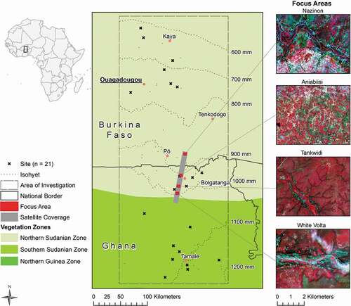
We selected four focus areas in the border region of Ghana and Burkina Faso, following the climate gradient (Figure 2). They were mainly chosen to capture variation along the climate gradient, in particular with respect to mean annual rainfall, which ranges from about 850 to 1000 mm a⁻¹ (Table 1). In this area, the rainy season lasts from June to September. The northernmost area covers part of the Nazinon river basin in Burkina Faso. Towards the south, it is followed by three areas in northern Ghana. These are Aniabiisi, located north-west of the city Bolgatanga; Tankwidi, covering parts of the Tankwidi river basin as well as the surrounding forest reserve; and White Volta, covering parts of the White Volta river basin. Vegetation belongs to the northern Sudanian savanna (White, 1983). The four focus areas also represent strong difference in land use. While the Aniabiisi area is intensively farmed and grazed by livestock (Berger et al., 2019), the three other areas located in river basins are characterized by more natural habitat conditions.

Table 1. Climatic and edaphic site conditions as well as main land cover types of the four focus areas in Burkina Faso and Ghana

Focus area	Country	Climate^a		Land cover^b	Edaphic conditions
		Mean annual temperature [°C]	Mean annual precipitation [mm]		Soil type^c	Sand content [%]^d	Silt content [%]^d	Clay content [%]^d
Nazinon	Burkina Faso	28.1	857.4	Open deciduous woodland, closed to open shrubland, agriculture	Cambisols	56.8	25.9	17.2
Aniabiisi	Ghana	28.3	923.8	Agriculture	Lixisols	53.4	29.6	17.0
Tankwidi	Ghana	28.4	981.3	Closed to open shrubland, grassland	Lixisols	61.8	22.2	15.9
White Volta	Ghana	28.3	1000.4	Closed to open shrubland	Lixisol	60.9	23.4	15.7

^awww.worldclim.org (Hijmans et al., 2005)

^bGessner et al. (2015)

^cHarmonized world soil database (FAO/IIASA/ISRIC/ISSCAS/JRC, 2012)

^dWorld soil Information (ISRIC, 2013)

Field data collection

For model calibration, we collected field data during the rainy season in 2012 at 21 sites spread along the north-south gradient (Figure 1(a)) that featured – as far as possible – different vegetation communities at varying phenological stages on diverse geological undergrounds and slope positions, as well as different intensities of grazing pressure. In this way, we intended to cover the whole range of the naturally occurring diversity of vegetation types within the research area. Spectral reflectance measurements of vegetation plots were performed using a FieldSpec 3 Hi-Res Portable Spectroradiometer (ASD Inc., Boulder, CO, USA) which detects light in a spectral range from 350 to 2500 nm (ASD Inc., 2006). Measurements were performed on 129 harvesting plots which were distributed over the 21 sampling sites. Plots had a circular shape and an area of ca. 0.25 m². For more details regarding the sampling design, see Ferner et al. (2015).

After measurements, aboveground plants vegetation was clipped to stubble height, air-dried and shipped to the laboratory of the Institute of Animal Science, University of Bonn (Germany). From the 129 samples taken in the field, several could not be used for model calibration due to partial sample losses and measurement errors. Lab analyses provided data (n > 100) for six forage variables. These are green biomass (gBM) as a measure of forage production (Ruppert & Linstädter, 2014), and a number of variables to characterize forage quality, that is, metabolisable energy (ME), acid detergent fibre (ADF), amylase-treated neutral detergent fibre (aNDF), ash, and phosphorus (P)). Samples were oven-dried (60°C, >48 h) to obtain dry mass, which equals gBM since only patches dominated by living vegetation were sampled. ME was determined based on in vitro gas production using the Hohenheim gas test (Menke & Steingass, 1988) as well as the sample’s crude protein content (for further details see Ferner et al. (2015)). ADF and aNDF were determined using an ANKOM2000 Fiber Analyzer (ANKOM Technology Corporation, Fairport, NY). Ash equals the residuals of the samples after incineration at a temperature of 550°C (method 8.1; VDLUFA (2012)) while P was determined using a spectrophotometer (method 10.6.1; VDLUFA (2012)).

Processing chain of satellite data

We evaluated the feasibility of models derived from hyperspectral near surface remote sensing to be upscaled to i) hyperspectral EO-1 Hyperion satellite imagery and ii) multispectral Sentinel-2 satellite imagery. Hyperion was mounted on the Earth-Observing 1 (EO-1) spacecraft (Ritchie et al., 1993) at 705 km above sea level. It provided 220 channels covering the visible and near-infrared portions of the solar spectrum from 350 to 2600 nm in 10 nm spectral resolution and 30 m spatial resolution. Hyperion was a pushbroom instrument that could image a 7.5 km by 100 km land area per image (Datt et al., 2003). Sentinel-2 is a constellation of two polar orbiting satellites equipped with an optical imaging sensor MSI (multi-spectral instrument; Brandt et al. (2015)). Here we used data from Sentinel-2A, which was launched on 23 June 2015. The satellite has 13 bands with a spatial resolution of 10 m – 60 m that span from the visible (VIS) and the near-infrared (NIR) to the short wave infrared (SWIR; Ky-Dembele et al. (2016)). Both satellites feature different sensor characteristics (Table 2).

Table 2. Summary of sensor characteristics of EO-1 Hyperion and Sentinel-2

Characteristic	EO-1 Hyperion	Sentinel-2
Launch date	21.11.2000	23.06.2015
Sensor resolution	hyperspectral	multispectral
Number of bands (bands used for this study)	242 (152)	13 (12)
Spatial/spectral resolution	30 m (0.4 to 2.5 µm)	10 m (band 2, 3, 4, 8/central wavelengths 492.4 nm, 559.8 nm, 664.6 nm, 832.8 nm) 20 m (band 5, 6, 7, 8A, 11, 12/central wavelengths 704.1 nm, 740.5 nm, 782.8 nm, 864.7 nm, 1613.7 nm, 2202.4 nm) 60 m (band 1, 9, 10/central wavelengths 442.7 nm, 945.1 nm, 1373.5 nm)
Quality	low signal-to-noise ratio	high signal-to-noise ratio
Availability	freely available; mainly on order (cloud-dependant image acquisition)	freely available; in combination with Sentinel-2B a revisit time of 5 days at the equator is achieved

Preprocessing of EO-1 Hyperion images

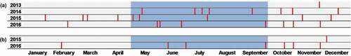
We acquired a time series of Hyperion images (26 in total; Figure 1(b)) covering at least the focus area of Aniabiisi from 2013 to 2016 (Figure 3(a)). All images were downloaded from USGS EarthExplorer (earthexplorer.usgs.gov) at a processing level of L1Gst (geometric systematic terrain corrected) or L1T (systematic terrain corrected).

Figure 3. Temporal coverage of (a) Hyperion and (b) Sentinel-2 time series available for Aniabiisi area in Upper East Region, Ghana, from 2013 to 2016. Dark areas indicate time of rainy season; bright areas indicate time of dry season

Hyperion data were delivered in a raw processing state and required several preprocessing steps to generate a product that could be used for monitoring purposes (see Figure 1). Preprocessing followed the procedure recommended by Rogass et al. (2014a), Rogass et al. (2014b)) and included a de-striping technique, half image SWIR shift as well as interpolation of dead pixels using smoothing and dead column substitution. Subsequently, bands from the VNIR and SWIR sensors were co-registered and a local log-polar phase correlation and best fit polynomial modelling applied. In a final step, images were spectrally smoothed using a Gaussian filter with sigma = 2. Afterwards all images were atmospherically corrected using ENVI FLAASH and lastly all bands affected by considerable noise (mostly due to atmospheric water vapour) were removed to leave 152 bands for further analysis.

Preprocessing of Sentinel-2 images

Sentinel-2 images were acquired for eight dates (December 2015 – December 2016; Figure 1(c)) to match ̶ as far as possible ̶ Hyperion image availability (Figure 3(b)). This was done to allow for a sound comparison of both sensor systems. Imagery was atmospherically corrected using the plugin “sen2cor” within the SNAP toolbox, provided by the European Space Agency (ESA). To match Hyperion spatial coverage, two separate Sentinel-2 tiles had to be mosaicked and clipped.

Spectral unmixing procedure

To assure that forage supply models were only applied to vegetated areas, a vegetation mask was created (Figure 1(d)). For this, we used MESMA (multiple endmember spectral mixture analysis; Dennison and Roberts (2003), Franke et al. (2009)) to determine the fractional cover of green vegetation on a pixel basis. We used a variety of pure field spectra of the three main land cover types in our study area, that is, photosynthetic active vegetation (PAV), non-photosynthetic active vegetation (NPAV) and open soil (SOIL), measured with the ASD Portable Spectroradiometer. Spectra were resampled in R (R Core Team, 2014) using the sensors´ spectral response functions to match spectral resolution of satellite images, that is, 152 bands for Hyperion and 12 bands for Sentinel-2. These spectra were used to create separate spectral libraries that served as input for MESMA calculation in Viper Tools, a plugin to ENVI developed by (Roberts et al., 2007). MESMA output was one image with fractional coverages of PAV, NPAV and SOIL as well as MESMA residuals.

Spectral model calibration to estimate forage supply

To evaluate the effects of different spectral resolutions on model performances, full-range field spectra had to be resampled in R using the sensor’s spectral response functions to match image spectral resolution (Figure 1(e)). Subsequently, we used the R package “autopls” (Schmidtlein et al., 2012) to apply partial least-squares regression with automated backward selection (PLSR; Wold et al. (2001)). Partial Least Squares Regression or Projection to Latent Structures is a multivariate regression method that is widely used in chemometrics, hyperspectral remote sensing, bioinformatics and other fields. PLSR is especially useful if the predictor variables are correlated or if the number of predictor variables is high as compared to the number of observations. The reason for this robustness is that the regression relies on a set of latent variables instead of the original, individual predictor variables. The latent variables form a feature space that is linearly related to the target variable as well as to the predictor variables.

Redundancy, noise and irrelevant or unreliable variables in the original predictor data set may nevertheless hamper the calibration process and lead to weak models. Therefore, several methods for selecting useful subsets of predictors have been proposed. Autopls consists of iterative runs of PLSR, each followed by a selection of predictors (here: reflectance in spectral bands at given locations). Root mean squared errors (RMSE) in cross-validation of the resulting values for the target variable (here: values for forage quality and quantity) are the criterion for choosing the next set. The iterations are repeated as long as a reduction of model errors or a reduction of the number of latent vectors can be achieved. For the final validation, leave-one-out cross-validation is used. The procedure was used to model the relations between resampled spectral data and all six forage variables, resulting in six final forage supply models.

The pre-processed images were masked to leave only pixels with a vegetation cover >30% (according to MESMA results). From the masked image, MESMA residuals were subtracted. This was done to receive natural spectral curves for each pixel, as we expected residuals to represent random noise. Finally, forage supply models were applied following Ferner et al. (2015) to obtain maps of estimated forage variables.

Linear model selection based on AIC

A Hyperion time-series from 2013 to 2016 was used to test the influence of five environmental predictors (i.e. phenology, precipitation, cumulative precipitation, land-use, and soil type) on forage characteristics, we used general linear models with a forward and backward model selection based on the Akaike information criterion (AIC). To test for the influence of phenology, a time series of MCD43A4 data was retrieved from the Moderate Resolution Imaging Spectroradiometer (MODIS), and NDVI values were calculated for the time period November 2013 to December 2016 as (NIR – Red)/(NIR + Red). We decided to use MODIS data due to its very high temporal resolution of one to two days which helped to get a high number of usable images even during the rainy season when clouds were frequent (Ferner et al., 2015). We then used the R package “phenex” to model daily NDVI values and to extract phenological parameters. These were date of green-up (the point where the function of modelled NDVI values first exceeded the threshold of 0.55), date of maximum NDVI, and date of senescence (the point where the function of modelled NDVI values first fell below 0.55). We used phenology as a factor with 1 = dates before green-up, 2 = dates between green-up and maximum NDVI, 3 = dates between maximum NDVI and senescence, and 4 = dates after senescence.

Precipitation was calculated per area as the monthly sum of rainfall (Schneider et al., 2011), using GPCC precipitation data provided by NOAA/OAR/ESRL PSD (via www.esrl.noaa.gov/psd/). Additionally, we included cumulative precipitation (cumPrecipitation) which equals the sum of precipitation of a given month plus the sum of the two preceding months. We also tested the main land use (1: open deciduous woodland, 2: closed to open shrubland, 3: agriculture) and soil types (1: cambisol, 2: lixisol; cf. Table 1). Model fits were determined using the adjusted coefficient of determination (adjR²) which corrects for the number of predictors in the model.

Results

Performances of PLSR models differed considerably between the three model types, that is, models using full-range field spectrometer data, models based on full-range data resampled to hyperspectral satellite resolution (Hyperion) and models resampled to multispectral satellite resolution (Sentinel-2) (Table 3).

Table 3. Summary of model fittings for all forage characteristics using partial least-squares regression. High adjR² values and low nRMSE values indicate a good fit of the regression models. Model validation was done via repeated (leave-one-out) cross validation (VAL_CV). The number of predictors (Pred) used for the respective latent variables (LV) is also given below

	Field spectrometer			Hyperion satellite			Sentinel-2 satellite
Forage characteristics	adjR^2	nRMSE [%]	LV (Pred)	adjR^2	nRMSE [%]	LV (Pred)	adjR^2	nRMSE [%]	LV (Pred)
	VALCV	VALCV		VALCV	VALCV		VALCV	VALCV
Green biomass (gBM)	0.66	10.86	6 (37)	0.36	12.28	7 (7)	0.42	11.82	5 (7)
Metabolisable energy (ME)	0.54	11.64	6 (32)	0.54	11.64	6 (23)	0.41	13.31	4 (6)
Amylase-treated neutral detergent fibre (aNDF)	0.45	12.68	7 (9)	0.48	12.25	9 (28)	0.27	14.37	11 (12)
Acid detergent fibre (ADF)	0.34	18.67	6 (15)	0.38	17.85	8 (13)	0.01	23.13	3 (12)
Phosphorus (P)	0.16	19.06	2 (33)	0.12	19.58	2 (7)	0.05	20.26	2 (12)
Ash	0.29	14.69	5 (7)	0.05	13.26	7 (92)	−0.10	14.69	2 (9)

Model fits revealed that not all forage characteristics could be successfully modelled. For Hyperion, models predicting P and ash achieved low model fits (_adjR² of 0.12 and 0.05, respectively), while spectral data resampled to Sentinel-2 resolution did not contain enough information to successfully model ADF, P and ash (_adjR² of 0.01, 0.05, and −0.1, respectively). To evaluate model plausibility and consistency between models, those bands selected for the models using the spectral resolution of the spectroradiometer, Hyperion and Sentinel-2 were compared (Figure 4).

Figure 4. Spectral bands (central wavelengths) selected for the models for (a) gBM, (b) ME, (c) aNDF, (d) ADF, (e) P, and (f) ash using the original spectral resolution of a field spectroradiometer as well as data resampled to match the spectral resolution of Hyperion and Sentinel-2. Bands were selected from different spectral regions, that is, visible region (VIS; 350–700 nm), near-infrared (NIR; 701–1300 nm), shortwave infrared I (SWIR I; 1301–1800 nm) and shortwave infrared II (SWIR II; 1801–2500 nm). Note that Sentinel-2 did not provide continuous spectral cover

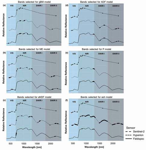
Many consistencies can be found between bands selected by different sensors. For gBM, the automatic band selection algorithm in autopls selected bands located in the NIR region while for ME, all models selected bands from the VIS region. For models predicting aNDF, selected bands were mainly located in the NIR (red edge) and SWIR II region. For ADF and P, many comparable bands from the SWIR and the NIR regions, respectively, were selected in the FieldSpec and the Hyperion model, while all available bands were selected in the Sentinel-2 model. The FieldSpec model predicting ash was quite similar to the model predicting P, while the Hyperion and Sentinel-2 models included numerous bands from almost all spectral regions.

Since only model fits for gBM, ME and aNDF achieved satisfactory results for all sensors, we concentrated our subsequent analyses on these forage characteristics. When applying the respective models to satellite imagery to generate forage supply maps, divergent results were achieved. Here, only maps for one time step (18./19.10.2016) are shown. These images provide data from the rainy season with a dense vegetation cover but only minimal cloud interference. For gBM (Figure 5), the pattern predicted by both satellite sensors closely matched for the intensively used area “Aniabiisi” (b). Here, areas with a high production of green biomass (see Figure 5(b)) often rendered forage with a low nutritive value (ME; see Figure 6(b)), and vice versa.

Figure 5. Forage supply map of green biomass (gBM) generated by applying models on Hyperion (18.10.16, left) and Sentinel-2 (19.10.16, right) imagery for the focus areas, i.e (a) Nazinon, (b) Aniabiisi, (c) Tankwidi, (d) White Volta

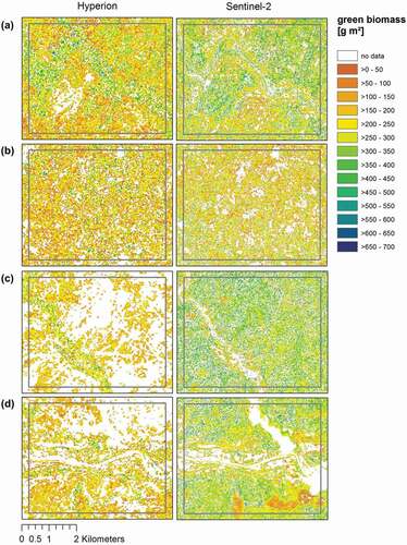
Figure 6. Forage supply map of metabolisable energy (ME) generated by applying models on Hyperion (18.10.16, left) and Sentinel-2 (19.10.16, right) imagery for the focus areas, that is, (a) Nazinon, (b) Aniabiisi, (c) Tankwidi, (d) White Volta

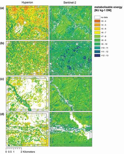
For the two southernmost regions “Tankwidi” (c) and “White Volta” (d), which are characterized by less arid conditions and near-natural vegetation, MESMA results differed, leading to many areas in the Hyperion image that were masked out before model application. The same applied for ME and aNDF models. A visual comparison with the original images (Figure 2) indicated that these masked areas were apparently covered by vegetation, that is, Sentinel-2 appears to produce better results. We assume that this is caused by considerable noise in the Hyperion image. For ME and aNDF, the agreement between both satellites is even lower, with Sentinel-2 estimating generally higher ME values (Figure 6) but lower aNDF values than Hyperion (see Figure A1 in Appendix).

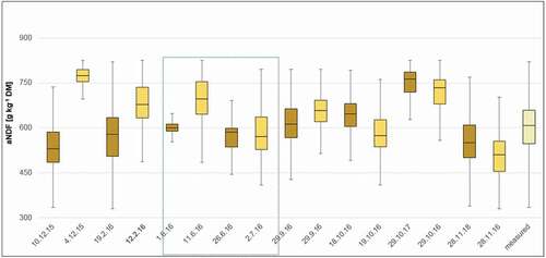
To better assess model plausibility, time series of modelled forage characteristics from all four focus areas (both from Hyperion and Sentinel-2 models) were compared to field-based data from the same vegetation zone, that is, Sudanian savanna. Vegetation samples were taken during the rainy season in summer 2012 (June – September). For all three forage characteristics, values estimated by Hyperion and Sentinel-2 models during the rainy season fall within the range of values measured in the lab so that both models generated plausible values (for comparison, the rainy season 2016 was marked with a blue coloured box; see Figures A2–A4 in Appendix).

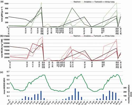
Over the course of the three growing seasons, dynamics of gBM and ME were clearly connected to seasonal changes between the dry and the rainy season (Figure 7). However, values varied widely between focus areas whereby values from the most northern/arid site Nazinon and the heavily grazed site Aniabiisi tended to be more similar. Based on the results of linear models, the overall effect of environmental drivers on the temporal development of forage characteristics were roughly comparable. Phenology exerted by far the most important influence, followed by cumulated precipitation sums over three months and recent precipitation, which was only a significant driver for ME (Table 4). The environmental drivers under consideration could model most forage characteristics with a fit higher than 0.43. Only the model for green biomass performed less well (adjR² = 0.34).

Table 4. Significance levels of environmental drivers chosen by stepwise (forward and backward) model selection for each forage characteristic. Phenology parameters were extracted from a MODIS NDVI time series, precipitation is the monthly sum of rainfall while cumulative precipitation (cumPrecipitation) equals the sum of precipitation of a given month plus the sum of the two preceding months. Land use (1: open deciduous woodland, 2: closed to open shrubland, 3: agriculture) and soil (1: cambisol, 2: lixisol; cf. Table 1) were also tested as predictors. High adjR² values indicate a good fit of the regression models

Forage characteristics (response variables)	Environmental drivers (predictors)					adjR^2
	Phenology	Precipitation	cumPrecipitation	Land use	Soil
Green biomass (gBM)	**		x		x	0.34
Metabolisable energy (ME)	***	*				0.43
Amylase-treated neutral detergent fibre (aNDF)	*		**			0.50
Acid detergent fibre (ADF)	**		*			0.45
Phosphorus (P)	**		*			0.46
Ash	**		*			0.43

Significance codes: “***” 0.001 “**” 0.01 “*” 0.05 “.” 0.1 ‘x’ 1

Figure 7. Seasonal dynamics of (a) total gBM and (b) ME for all four focus areas predicted based on Hyperion time series. Areas affected by cloud cover were excluded. For comparison, (c) seasonal dynamics of MODIS NDVI time series used for the extraction of phenology parameters and sum of precipitation averaged over all four focus areas are shown

Discussion

Performance of resampled forage models – the spectral aspect

A main aim of this study was to model forage characteristics from in-situ hyperspectral data resampled to match the spectral resolution of multi- and hyperspectral satellites. Here, we first discuss how spectral characteristics of Sentinel-2 and Hyperion sensors influenced model performance.

To answer this question, we developed an elaborate methodology which implied resampling the sensor’s spectral response functions to match image spectral resolution, and using partial least squares regression (PLSR) for model calibration. PLSR was chosen due to its ability to deal with the high dimensionality and collinearity of hyperspectral data (Carrascal et al., 2009) while retaining only significant components with a high explanatory power (Harsanyi & Chang, 1994). We found that, for all tested spectral resolutions, our methodological approach was successful in calibrating models for three forage characteristics (gBM, ME, and aNDF).

With respect to wavelengths selected by PLSR, successful models shared many similarities, which supports the idea of a causal relationship between selected spectral regions and the forage characteristic under investigation (Knox et al., 2012). Examples of these similarities include the selection of bands from the NIR region (especially 800–900 nm) for gBM, for example, Sentinbel-2 bands 8 (centred at 832.8 nm) and 8A (centred at 864.7 nm), whereby the latter was also chosen in a study by Sibanda et al. (2015) predicting grass biomass and relates to the vegetation´s biophysical quantity and yield (Thenkabail et al., 2013). Additionally, all ME models selected bands from the VIS region (350–700 nm), including Sentinel-2 bands 1 (centred at 442.7 nm) and 3 (centred at 559.8 nm) which relate to chlorophyll concentration (Curran, 1989). All models predicting aNDF selected bands from the red edge and SWIR II region. Sentinel-2´s red edge bands (band 5–7) are cantered in the 700–800 nm region. It is not surprising that this region, which is strongly affected by the vegetation’s vitality, proved to be important to model an age-dependent plant characteristic such as fibre. On the other hand, Sentinel-2 band 12 (centred at 2202.4 nm) in the SWIR II region is quite broad and covers different adsorption features of starch, cellulose but also protein and nitrogen (Curran, 1989).

A comparably lower predictive power was observed for the Sentinel-2 models aimed at predicting aNDF. We assume that this is due to the missing spectral coverage of the Sentinel-2 sensor in the SWIR II region. Hence, while the FieldSpec and Hyperion models selected several SWIR II bands for aNDF prediction, only one band was available in Sentinel-2 models. Likewise, the low predictive power of the Sentinel-2 model for ADF could be explained by the insufficient spectral resolution of Sentinel-2 in the SWIR I and SWIR II region. Although the SWIR I band (related to lignin, but also starch, protein and nitrogen (Curran, 1989)) and SWIR II band (related to protein and nitrogen (Curran, 1989)) of Sentinel-2 are well placed to detect some important forage information, they still provide only data from two bands from a very broad spectral area which contains manifold important information for forage studies (Card et al., 1988; Curran, 1989; Norris et al., 1976; Workman & Weyer, 2008).

Our attempts to model P were not successful, neither for the full spectral resolution provided by the field spectroradiometer, nor for the satellite resolutions. In general, P concentrations in the soil of the research area are very low (Guuroh et al., 2018; Nwoke et al., 2003). Therefore, spectral adsorption features of more frequent constituents like water, cellulose, and nitrogen might have hindered the detection of P (Kokaly et al., 2009). In addition, inorganic compounds cannot be detected directly via field spectroscopy, but only if a correlation exists with detectable organic compounds or structural plant characteristics (Deaville & Flinn, 2000; Reeves, 2000). Such a correlation was not found for our dataset (results not shown).

Likewise, our attempts to model ash failed, since the band selection procedure failed to select meaningful bands. Even in most of our models based on hyperspectral data, the algorithm selected only a few bands, possibly due to the high multicollinearity of hyperspectral data (Clevers et al., 2007; De Jong et al., 2003). It can be concluded that the low number of broad bands of Sentinel-2 in the SWIR region reduced the predictive power of many forage models in comparison to those based on hyperspectral data (Mansour et al., 2012). However, in general the spectral coverage of Sentinel-2 proved to be sufficiently high and strategically well placed for rangeland monitoring and management purposes (Sibanda et al., 2016).

Application of models on satellite data – the spatial aspect

A second aim of our study was to assess the transferability of field-developed statistical models to satellite imagery, with the idea to create spatial information in the form of forage maps. To ensure this transferability, we developed a multi-step methodology to avoid common obstacles during the upscaling procedure. We first applied a mask based on MESMA results to ensure that models were only applied on vegetated pixels. The idea of such a mask was already suggested by Coops et al. (2003) and realized by, for example, Suzuki et al. (2012) and Psomas et al. (2011). The fact that modelled forage characteristics fell all within the range of those measured in the field are a strong indication of our success. Hence, our results underline the importance of a well-designed preprocessing (and not postprocessing) step to improve a match of targets (here vegetation) between model calibration and model application, since it can never be assured that the model does not predict reasonable values when applied on incongruous targets, for example, soil pixels.

Furthermore, for upscaling field-based spectrometric measurements to satellite data, it is mandatory to convert at-sensor radiance to surface reflectance by applying atmospheric correction (Psomas et al., 2011). Such a procedure is also prerequisite for multi-scene and multi-date analysis. Due to software limitations, we had to apply two different atmospheric correction methods to Hyperion and Sentinel-2 images, which might have caused some observed differences in pixel values and thus model outcomes (Martin et al., 2008). Both abovementioned aspects have to be carefully considered when transferring field-developed statistical models to satellite imagery.

Furthermore, our study aimed at elucidating how the sensor type (hyperspectral vs. multispectral) would affect model transfer to satellite data. When comparing the performance of Hyperion and Sentinel-2, it became clear that none of the tested satellites provided optimal characteristics for the purpose of regular forage supply monitoring in subtropical savanna grassland. We tested Hyperion as a representative of a hyperspectral satellite, since it was the only satellite providing repeatedly and freely available hyperspectral imagery at the time of the study. Hyperion has several major shortcomings, including a low signal-to-noise ratio, unpredictable image acquisition, varying image coverage and the fact that the satellite was deactivated on 30 March 2017. The low data quality of the sensor became obvious in the grainy model results despite complex image preprocessing. In comparison to Sentinel-2 models, though, Hyperion’s higher spectral resolution led to a higher model fit and lower prediction error for five of the six tested forage characteristics. Our results support the idea that a higher spectral coverage contains more essential information about plant constituents and thus enables the calibration of better fitted models for flexible application opportunities (Durante et al., 2014). For future applications, a number of hyperspectral satellites will be available, for example, Copernicus Hyperspectral Imaging Mission for the Environment (CHIME), PRISMA, EnMAP HyperSpectral Imager, HISUI, Spaceborne Hyperspectral Applicative Land and Ocean Mission (SHALOM), Hyperspectral Infrared Imager (HyspIRI) and Hyperspectral X IMagery (HypXIM) (Transon et al., 2018).

Until these new satellites are operational, especially for applications in Africa, more practical and affordable multispectral remote sensing alternatives are needed (Zengeya et al., 2013). With the launch of Sentinel-2B on 7 March 2017, a frequent image acquisition (i.e. every five days) is possible, offering optimal conditions for monitoring purposes based on freely available imagery. The strategically placed bands of Sentinel 2, especially in the red-edge region, facilitate estimates of chemical constituents and can partly compensate for the reduced data range compared to hyperspectral sensors (Ramoelo et al., 2012).

Our comparison of forage supply maps based on multi- and hyperspectral satellites rendered considerable differences. As predicted data ranges from both sensors fell within the range of the samples taken on the ground, we are not able to determine which satellite provided better estimates. However, forage maps based on Sentinel-2 data tended to be visually more plausible since the MESMA procedure masked only non-vegetated areas and the spatial pattern of forage characteristics were less noisy than with Hyperion. A future satellite system should ideally combine the advantages of both tested data sources to install a more reliable monitoring system, i.e. the high spectral resolution of Hyperion and the high data quality and availability of Sentinel-2. The EnMAP sensor has a great potential to fill this gap in the future. It is supposed to provide a high spectral coverage (420 to 2450 nm) in combination with a low signal-to-noise ratio at a spatial resolution of 30 m (Guanter et al., 2015). Also, like the Sentinel satellites, it will offer a high revisit time of up to four days at the equator as well as cost-free images for scientific use (Guanter et al., 2015). More recently, it became clear that ESA’s planned CHIME satellite in the Sentinel family might provide even more suitable characteristics for regular forage supply monitoring (Nieke & Rast, 2018).

Drivers of regional forage resources – the ecological aspect

Our final study aim was to match spatio-temporal patterns in forage characteristics to patterns in environmental drivers to gain an improved understanding of forage resource dynamics. Our results indicate that both forage quantity (green biomass) and forage quality (as captured by ME and aNDF) varied considerably in time and space. This expected result is in line with previous remote sensing studies from grasslands (e.g. Beeri et al., 2007; Durante et al., 2014; Levick & Rogers, 2011; Suzuki et al., 2012). We also found that areas with high biomass production often (but not always) rendered forage with a low quality, and vice versa. These observations can be explained by inherent trade-offs between forage quantity and forage quality (Mueller et al., 2008). Therefore, we recommend considering both, the quantity but also the quality of forage when looking for monitoring approaches that support a resilient use of forage resources in the face of global change.

To cover two potentially important environmental drivers of forage supply, that is, climate and land-use, our study design captured steep gradients of climatic aridity and grazing pressure. However, at the broad spatial scale considered in this study, only general conclusions about regional drivers of forage supply can be drawn. In agreement with earlier studies [e.g. Grant and Scholes (2006), Knox et al. (2012)], we found pronounced seasonal changes in forage supply between the wet and dry season. As expected for a dryland region, seasonal dynamics of forage supply were found to be closer connected to rainfall patterns than to grazing intensities (Kgosikoma et al., 2015).

We found that both the most arid focus area (Nazinon) and the most heavily grazed area (Aniabiisi) had the tendency for a higher forage quality. Arid areas support the growth of annual plants (Hempson et al., 2015) which often feature a high forage quality (Le Houérou, 1980). Likewise, high grazing pressure in savanna grasslands can induce a dominance shift from perennial to annual plants (Fuhlendorf & Engle, 2001; Pfeiffer et al., 2019). This supports the idea of aridity and grazing exerting convergent selective forces on plants (Reeves, 2000), as found by Linstädter et al. (2014) in an earlier study from African savanna grasslands. Furthermore, a shift of plant communities towards highly nutritious “grazing lawns” with a high grazing value can be observed under intensive grazing impact (Hempson et al., 2015). High grazing pressure can stimulate the regrowth of fresh palatable plant material, thus keeping vegetation in an early phenological stage (Moreno García et al., 2014).

In this regard, it is not surprising that plant phenology, which is functionally linked to a progressive decline in digestibility and crude protein (Changwony et al., 2015), was found to be the most important predictor of forage characteristics. Cumulative precipitation, in contrast to precipitation, integrates the recent history of rainfall events over the last three months. A study in the same research area but at a finer spatial resolution found antecedent rainfall to be an important driver of forage biomass (Guuroh et al., 2018). We assume that cumulative precipitation, in contrast to recent precipitation, is a better proxy of current ground water levels which in turn influence plant growth. In addition, cumulative precipitation can modulate the rivers’ water levels within our focus areas and thus forage resources on river banks (Nilsson & Svedmark, 2002). These areas are of special importance for pastoralists since they show consistently earlier green-up and delayed senescence and thus act as key pastoral forage sites (Brottem et al., 2014).

An earlier field-based study from the same research area that was restricted to the rainy season revealed that local-scale forage supply was mainly controlled directly by land-use intensity, including fire frequency and grazing pressure. However, indirect proxies like aridity, vegetation characteristics and weather fluctuations also played a role (Ferner et al., 2018). Both studies agree that vegetation dynamics and water availability play an important role in explaining forage supply. On the broader spatial and temporal scales of this study, however, the substantial temporal changes due to the phenological development of plants and the influence of seasonal shifts between dry and rainy seasons may have overridden the more local influence of land-use drivers. A certain information loss thus seems to be inevitable when the aim is to be independent of resource-intensive local measurements and to provide information on larger scale instead.

Limitations of our approach

Our data sampling approach ensured a direct relationship between the spectral reflectance of vegetation and the samples analysed in the lab. However, this was only possible for relatively small sampling plots (i.e. 0.25 m²) while other studies have emphasized the importance of a match between field and remote sensing image sampling resolutions (e.g. Thulin et al. (2012)). This approach was not suitable in our case for four reasons. First, the investigated satellites featured different spatial resolutions; second, an estimation of ME is very costly and could not be provided for a representative area of a 30 × 30 m pixel; third, Hyperion image acquisition was not predictable but depended on weather forecasts; and fourth, the flight height and spatial coverage of the Hyperion satellite varied over time.

A further limitation of this approach is that no truly independent validation of model results was possible and we rely instead on an internal cross-validation procedure. With respect to the robustness and transferability of resampled models, Mutanga et al. (2015) found that although the model performance of resampled spectral data tended to overestimate model accuracy in comparison to a real application on satellite data, the magnitude of errors due to the up-scaling procedure was small enough to support a transfer. These results provide a legitimation of our approach, and give us confidence that our study rendered robust and transferable results. Nonetheless, we emphasise the need to further investigate model performance based on independent validation plots on the ground, which would only be possible for Sentinel-2 models. Furthermore, we acknowledge that testing other regression methods (e.g. random forest) or using vegetation indices in addition to reflectance data might have resulted in better model fits. However, testing different regression methods was beyond the scope of our study which focused on comparing the usability of multi- and hyperspectral data. In this context, we expect our results to further improve by adding free Landsat 8 and future Landsat 9 images to the analysis, as supported by other studies [e.g. Sibanda et al. (2015), Forkuor et al. (2018), and Wang et al. (2019)].

Our four focus areas differed with respect to habitat characteristics such as the presence of rivers or forests. Trees can dominate remote sensing based time-series analyses in this area (Brandt et al., 2015), but at the spatial resolution of Hyperion images we were not able to specifically mask out trees. Since leaves provide an important source of forage, especially during the dry season (Ky-Dembele et al., 2016), and the riparian zone provides highly nutritious grasses (Ramoelo et al., 2012) irrespective of the rainy season, we refrained from excluding floodplains. However, our models were specifically calibrated on herbaceous vegetation and an application on pixels dominated by tree spectra might have decreased model reliability in these areas.

The time series considered in our study ended in 2016, since Hyperion images showed an increasing level of noise prior to the deactivation of the satellite on 30 March 2017. As a result, data for a direct comparison of Hyperion and Sentinel-2 (launch date: 23 June 2015 with first images being available in autumn 2015) were only available for a time span of ca. one year. This might have decreased the explanatory power of our analysis. Moreover, it did not allow for a temporal assessment of multi- and hyperspectral model results. However, all seasons as well as very different habitat types were covered which ensured the validity of our conclusions.

Conclusion

While numerous studies have investigated the potential applications of near-surface remote sensing in detecting essential chemical constituents of vegetation, few studies have used this method to create maps based on satellite or aerial images in order to tackle urgent ecological challenges. Our study presents an attempt to go one step further to directly use remote sensing products, aided by field spectroscopy, in order to determine important drivers of forage supply in an African savanna grassland. Our findings provide evidence that partial least-squares regression is able to model several important forage characteristics based on hyperspectral as well as multispectral data. However, generated maps differed considerably: While the high spectral resolution of Hyperion imagery allowed for improved model fits, the better quality of Sentinel-2 images resulted in more realistic maps of forage characteristics. We therefore conclude that so far none of the tested sensors provide optimal features for a regular forage monitoring. In the future, several planned hyperspectral missions will likely fill this gap. Nonetheless, by using a time-series of Hyperion images, we were able to contribute to a better understanding of forage drivers at a regional scale. Future research in this regard should focus on more reliable model validation methods to adequately evaluate model performances before eventually installing automated monitoring systems of forage supply.

Acknowledgments

This study was funded by the German Federal Ministry of Education and Research (BMBF) through the WASCAL initiative (FKZ 01LG1202A). AL also acknowledges funding through the WASCAL WRAP 2.0 initiative (GreenGaDe project, grant 01LG2078A). We are grateful to all farmers who granted us access to their rangelands. Our thanks also go to Reginald Guuroh and Kristijan Čanak for helpful discussions, Gohar Ghazaryan for the provision of the NDVI time series, and to Joanna Pardoe for improving the English.

Data availability statement

The data that support the findings of this study are available from the corresponding author, JF, upon reasonable request.

Disclosure statement

No potential conflict of interest was reported by the author(s).

Additional information

Funding

This work was supported by the German Federal Ministry of Education and Research (BMBF) through WASCAL and the WASCAL WRAP 2.0 project GreenGaDe; Bundesministerium für Bildung und Forschung [01LG1202A,01LG2078A];

Appendix

Figure A1. Forage supply map of amylase-treated neutral detergent fibre (aNDF) generated by applying models on Hyperion (18.10.16, left) and Sentinel-2 (19.10.16, right) imagery for the focus areas, that is, (a) Nazinon, (b) Aniabiisi, (c) Tankwidi, (d) White Volta

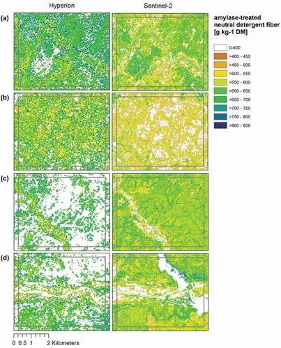
Figure A2. Box plots reflecting the time series of green biomass (gBM) values from the four focus areas predicted from Hyperion (dark colour) and Sentinel-2 (light colour) images in comparison to field samples measured during the rainy season 2012 (box plot to the right). The time period of the rainy season 2016 (June – Sept 2016) is marked with a box

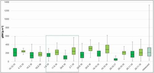
Figure A3. Box plots reflecting the time series of metabolisable energy (ME) values from the four focus areas predicted from Hyperion (dark colour) and Sentinel-2 (light colour) images in comparison to field samples measured during the rainy season 2012 (box plot to the right). The time period of the rainy season 2016 (June – Sept 2016) is marked with a box

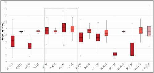
Figure A4. Box plots reflecting the time series of amylase-treated neutral detergent fibre (aNDF) values from the four focus areas predicted from Hyperion (dark colour) and Sentinel-2 (light colour) images in comparison to field samples measured during the rainy season 2012 (box plot to the right). The time period of the rainy season 2016 (June – Sept 2016) is marked with a box

References

- Abraham, J. O., Hempson, G. P., & Staver, A. C. (2019). Drought‐response strategies of savanna herbivores. Ecology and Evolution, 9(12), 7047–7056. https://doi.org/https://doi.org/10.1002/ece3.5270
- Anderson, M. C., Neale, C. M. U., Li, F., Norman, J. M., Kustas, W. P., Jayanthi, H., & Chavez, J. (2004). Upscaling ground observations of vegetation water content, canopy height, and leaf area index during SMEX02 using aircraft and Landsat imagery. Remote Sensing of Environment, 92(4), 447–464. https://doi.org/https://doi.org/10.1016/j.rse.2004.03.019
- Anyamba, A., & Tucker, C. J. (2005). Analysis of Sahelian vegetation dynamics using NOAA-AVHRR NDVI data from 1981-2003. Journal of Arid Environments, 63(3), 596–614. https://doi.org/https://doi.org/10.1016/j.jaridenv.2005.03.007
- ASD Inc. (2006). FieldSpec® 3 Spectroradiometer - user’s manual. Analytical Spectral Devices, Inc.
- Asner, G. P. (1998). Biophysical and biochemical sources of variability in canopy reflectance. Remote Sensing of Environment, 64(3), 234–253. https://doi.org/https://doi.org/10.1016/S0034-4257(98)00014-5
- Beeri, O., Phillips, R., Hendrickson, J., Frank, A. B., & Kronberg, S. (2007). Estimating forage quantity and quality using aerial hyperspectral imagery for northern mixed-grass prairie. Remote Sensing of Environment, 110(2), 216–225. https://doi.org/https://doi.org/10.1016/j.rse.2007.02.027
- Berger, S., Bliefernicht, J., Linstädter, A., Canak, K., Guug, S., Heinzeller, D., Hingerl, L., Mauder, M., Neidl, F., Quansah, E., Salack, S., Steinbrecher, R., & Kunstmann, H. (2019). The impact of rain events on CO2 emissions from contrasting land use systems in semi-arid West African savannas. Science of the Total Environment, 647, 1478–1489. https://doi.org/https://doi.org/10.1016/j.scitotenv.2018.07.397
- Boone, R. B., Conant, R. T., Sircely, J., Thornton, P. K., & Herrero, M. (2017). Climate Change Impacts on Selected Global Rangeland Ecosystem Services. Global Change Biology, 24(3), 1382–1393. https://doi.org/https://doi.org/10.1111/gcb.13995
- Brandt, M., Mbow, C., Diouf, A. A., Verger, A., Samimi, C., & Fensholt, R. (2015). Ground- and satellite-based evidence of the biophysical mechanisms behind the greening Sahel. Global Change Biology, 21(4), 1610–1620. https://doi.org/https://doi.org/10.1111/gcb.12807
- Brottem, L., Turner, M. D., Butt, B., & Singh, A. (2014). Biophysical variability and pastoral rights to resources: West African transhumance revisited. Human Ecology, 42(3), 351–365. https://doi.org/https://doi.org/10.1007/s10745-014-9640-1
- Brüser, K., Feilhauer, H., Linstädter, A., Schellberg, J., Oomen, R. J., Ruppert, J. C., & Ewert, F. A. (2014). Discrimination and characterization of management systems in semi-arid rangelands of South Africa using RapidEye time series. International Journal of Remote Sensing, 35(5), 1653–1673. https://doi.org/https://doi.org/10.1080/01431161.2014.882028
- Card, D. H., Peterson, D. L., Matson, P. A., & Aber, J. D. (1988). Prediction of Leaf Chemistry by the Use of Visible and near-Infrared Reflectance Spectroscopy. Remote Sensing of Environment, 26(2), 123–147. https://doi.org/https://doi.org/10.1016/0034-4257(88)90092-2
- Carrascal, L. M., Galvan, I., & Gordo, O. (2009). Partial least squares regression as an alternative to current regression methods used in ecology. Oikos, 118(5), 681–690. https://doi.org/https://doi.org/10.1111/j.1600-0706.2008.16881.x
- Changwony, K., Alvarez, M., Lanyasunya, T. P., Dold, C., Becker, M., & Südekum, K.-H. (2015). Biomass and quality changes of forages along land use and soil type gradients in the riparian zone of Lake Naivasha, Kenya. Ecological Indicators, 49, 169–177. https://doi.org/https://doi.org/10.1016/j.ecolind.2014.10.013
- Cho, M. A., Skidmore, A., Corsi, F., Van Wieren, S. E., & Sobhan, I. (2007). Estimation of green grass/herb biomass from airborne hyperspectral imagery using spectral indices and partial least squares regression. International Journal of Applied Earth Observation and Geoinformation, 9(4), 414–424. https://doi.org/https://doi.org/10.1016/j.jag.2007.02.001
- Clevers, J. G. P. W., Van Der Heijden, G. W. A. M., Verzakov, S., & Schaepman, M. E. (2007). Estimating grassland biomass using SVM band shaving of hyperspectral data. Photogrammetric Engineering and Remote Sensing, 73(10), 1141–1148. https://doi.org/https://doi.org/10.14358/PERS.73.10.1141
- Coops, N. C., Smith, M. L., Martin, M. E., & Ollinger, S. V. (2003). Prediction of eucalypt foliage nitrogen content from satellite-derived hyperspectral data. Ieee Transactions on Geoscience and Remote Sensing, 41(6), 1338–1346. https://doi.org/https://doi.org/10.1109/TGRS.2003.813135
- Curran, P. J. (1989). Remote sensing of foliar chemistry. Remote Sensing of Environment, 30(3), 271–278. https://doi.org/https://doi.org/10.1016/0034-4257(89)90069-2
- Datt, B., McVicar, T. R., Van Niel, T. G., Jupp, D. L. B., & Pearlman, J. S. (2003). Preprocessing EO-1 Hyperion hyperspectral data to support the application of agricultural indexes. Ieee Transactions on Geoscience and Remote Sensing, 41(6), 1246–1259. https://doi.org/https://doi.org/10.1109/TGRS.2003.813206
- De Jong, S. M., Pebesma, E. J., & Lacaze, B. (2003). Above-ground biomass assessment of Mediterranean forests using airborne imaging spectrometry: The DAIS Peyne experiment. International Journal of Remote Sensing, 24(7), 1505–1520. https://doi.org/https://doi.org/10.1080/01431160210145560
- Deaville, E. R., & Flinn, P. C. (2000). Near-infrared (NIR) spectroscopy: An alternative approach for the estimation of forage quality and voluntary intake. In D.I. Givens, E. Owen, R.F.E. Axford, & H.M. Omed (Eds.), Forage evaluation in ruminant nutrition. (pp. 301–320). CAB International.
- Dennison, P. E., & Roberts, D. A. (2003). Endmember selection for Multiple Endmember Spectral Mixture Analysis using endmember average RSME. Remote Sensing of Environment, 87(2–3), 123–135. https://doi.org/https://doi.org/10.1016/S0034-4257(03)00135-4
- Diallo, O., Diouf, A., Hanan, N. P., Ndiaye, A., & Prevost, Y. (1991). Avhrr monitoring of savanna primary production in Senegal, West Africa - 1987-1988. International Journal of Remote Sensing, 12(6), 1259–1279. https://doi.org/https://doi.org/10.1080/01431169108929725
- Durante, M., Oesterheld, M., Pineiro, G., & Vassallo, M. M. (2014). Estimating forage quantity and quality under different stress and senescent biomass conditions via spectral reflectance. International Journal of Remote Sensing, 35(9), 2963–2981. https://doi.org/https://doi.org/10.1080/01431161.2014.894658
- Duru, M., Jouany, C., Theau, J. P., Granger, S., & Cruz, P. (2015). A plant-functional-type approach tailored for stakeholders involved in field studies to predict forage services and plant biodiversity provided by grasslands. Grass and Forage Science, 70(1), 2–18. https://doi.org/https://doi.org/10.1111/gfs.12129
- Egeru, A., Wasonga, O., Mburu, J., Yazan, E., Majaliwa, M. G. J., MacOpiyo, L., & Bamutaze, Y. (2015). Drivers of forage availability: An integration of remote sensing and traditional ecological knowledge in Karamoja sub-region, Uganda. Pastoralism, 5(1), 1–18. https://doi.org/https://doi.org/10.1186/s13570-015-0037-6
- FAO/IIASA/ISRIC/ISSCAS/JRC. (2012). Harmonized World Soil Database (version 1.2). FAO.
- Ferner, J., Linstädter, A., Südekum, K.-H., & Schmidtlein, S. (2015). Spectral indicators of forage quality in West Africa’s tropical savannas. International Journal of Applied Earth Observation and Geoinformation, 41, 99–106. https://doi.org/https://doi.org/10.1016/j.jag.2015.04.019
- Ferner, J., Schmidtlein, S., Guuroh, R. T., Lopatin, J., & Linstädter, A. (2018). Disentangling effects of climate and land-use change on West African drylands’ forage supply. Global Environmental Change, 53, 24–38. https://doi.org/https://doi.org/10.1016/j.gloenvcha.2018.08.007
- Forkuor, G., Dimobe, K., Serme, I., & Tondoh, J. E. (2018). Landsat-8 vs. Sentinel-2: Examining the added value of sentinel-2’s red-edge bands to land-use and land-cover mapping in Burkina Faso. Giscience & Remote Sensing, 55(3), 331–354. https://doi.org/https://doi.org/10.1080/15481603.2017.1370169
- Franke, J., Roberts, D. A., Halligan, K., & Menz, G. (2009). Hierarchical Multiple Endmember Spectral Mixture Analysis (MESMA) of hyperspectral imagery for urban environments. Remote Sensing of Environment, 113(8), 1712–1723. https://doi.org/https://doi.org/10.1016/j.rse.2009.03.018
- Fuhlendorf, S. D., & Engle, D. M. (2001). Restoring heterogeneity on rangelands: Ecosystem management based on evolutionary grazing patterns. Bioscience, 51(8), 625–632. https://doi.org/https://doi.org/10.1641/0006-3568(2001)051[0625:RHOREM]2.0.CO;2
- Fynn, R. W. S., Augustine, D. J., Peel, M. J. S., & De Garine-wichatitsky, M. (2016). Strategic management of livestock to improve biodiversity conservation in African savannahs: A conceptual basis for wildlife–livestock coexistence. Journal of Applied Ecology, 53(2), 388–397. https://doi.org/https://doi.org/10.1111/1365-2664.12591
- Gaitan, J. J., Oliva, G. E., Bran, D. E., Maestre, F. T., Aguiar, M. R., Jobbagy, E. G., Buono, G. G., Ferrante, D., Nakamatsu, V. B., Ciari, G., Salomone, J. M., & Massara, V. (2014). Vegetation structure is as important as climate for explaining ecosystem function across Patagonian rangelands. Journal of Ecology, 102(6), 1419–1428. https://doi.org/https://doi.org/10.1111/1365-2745.12273
- Gessner, U., Machwitz, M., Esch, T., Tillack, A., Naeimi, V., Kuenzer, C., & Dech, S. (2015). Multi-sensor mapping of West African land cover using MODIS, ASAR and TanDEM-X/TerraSAR-X data. Remote Sensing of Environment, 164, 282–297. https://doi.org/https://doi.org/10.1016/j.rse.2015.03.029
- Grant, C. C., & Scholes, M. C. (2006). The importance of nutrient hot-spots in the conservation and management of large wild mammalian herbivores in semi-arid savannas. Biological Conservation, 130(3), 426–437. https://doi.org/https://doi.org/10.1016/j.biocon.2006.01.004
- Guanter, L., Kaufmann, H., Segl, K., Foerster, S., Rogass, C., Chabrillat, S., Kuester, T., Hollstein, A., Rossner, G., Chlebek, C., Straif, C., Fischer, S., Schrader, S., Storch, T., Heiden, U., Mueller, A., Bachmann, M., Mühle, H., Müller, R., Habermeyer, M., … Sang, B. (2015). The EnMAP Spaceborne Imaging Spectroscopy Mission for Earth Observation. Remote Sensing, 7(7), 8830–8857. https://doi.org/https://doi.org/10.3390/rs70708830
- Guuroh, R. T., Ruppert, J. C., Ferner, J., Čanak, K., Schmidtlein, S., & Linstädter, A. (2018). Drivers of forage provision and erosion control in West African savannas — A macroecological perspective. Agriculture, Ecosystems & Environment, 251, 257–267. https://doi.org/https://doi.org/10.1016/j.agee.2017.09.017
- Hansen, P. M., & Schjoerring, J. K. (2003). Reflectance measurement of canopy biomass and nitrogen status in wheat crops using normalized difference vegetation indices and partial least squares regression. Remote Sensing of Environment, 86(4), 542–553. https://doi.org/https://doi.org/10.1016/S0034-4257(03)00131-7
- Harsanyi, J. C., & Chang, C. (1994). Hyperspectral image classification and dimensionality reduction: An orthogonal subspace projection approach. Ieee Transactions on Geoscience and Remote Sensing, 32(4), 779–785. https://doi.org/https://doi.org/10.1109/36.298007
- Hempson, G. P., Archibald, S., Bond, W. J., Ellis, R. P., Grant, C. C., Kruger, F. J., Kruger, L. M., Moxley, C., Owen-Smith, N., Peel, M. J. S., Smit, I. P. J., & Vickers, K. J. (2015). Ecology of grazing lawns in Africa. Biological Reviews, 90(3), 979–994. https://doi.org/https://doi.org/10.1111/brv.12145
- Hijmans, R. J., Cameron, S. E., Parra, J. L., Jones, P. G., & Jarvis, A. (2005). Very high resolution interpolated climate surfaces for global land areas. International Journal of Climatology, 25(15), 1965–1978. https://doi.org/https://doi.org/10.1002/joc.1276
- Huang, J., Yu, H., Guan, X., Wang, G., & Guo, R. (2016). Accelerated dryland expansion under climate change. Nature Climate Change, 6(2), 166. https://doi.org/https://doi.org/10.1038/nclimate2837
- IPCC. 2019. Climate Change and Land. An IPCC Special Report on climate change, desertification, land degradation, sustainable land management, food security, and greenhouse gas fluxes in terrestrial ecosystems. Intergovernmental Panel on Climate Change.
- ISRIC. 2013. World Soil Information, 2013. Soil property maps of Africa at 1 km. Available for download at www.isric.org.
- Kgosikoma, O. E., Mojeremane, W., & Harvie, B. (2015). The impact of livestock grazing management systems on soil and vegetation characteristics across savanna ecosystems in Botswana. African Journal of Range & Forage Science, 1–8.
- Knox, N. M., Skidmore, A. K., Prins, H. H. T., Asner, G. P., Van Der Werff, H. M. A., De Boer, W. F., Van Der Waal, C., De Knegt, H. J., Kohi, E. M., Slotow, R., & Grant, R. C. (2011). Dry season mapping of savanna forage quality, using the hyperspectral Carnegie Airborne Observatory sensor. Remote Sensing of Environment, 115(6), 1478–1488. https://doi.org/https://doi.org/10.1016/j.rse.2011.02.007
- Knox, N. M., Skidmore, A. K., Prins, H. H. T., Heitkönig, I. M. A., Slotow, R., Van Der Waal, C., & De Boer, W. F. (2012). Remote sensing of forage nutrients: Combining ecological and spectral absorption feature data. Isprs Journal of Photogrammetry and Remote Sensing, 72, 27–35. https://doi.org/https://doi.org/10.1016/j.isprsjprs.2012.05.013
- Kokaly, R. F., Asner, G. P., Ollinger, S. V., Martin, M. E., & Wessman, C. A. (2009). Characterizing canopy biochemistry from imaging spectroscopy and its application to ecosystem studies. Remote Sensing of Environment, 113, S78–S91. https://doi.org/https://doi.org/10.1016/j.rse.2008.10.018
- Kooistra, L., Barranco, M., Van Dobben, H., & Schaepman, M. 2006. Regional scale monitoring of vegetation biomass in river floodplains using imaging spectroscopy and ecological modeling. 124–127 in 2006 IEEE International Symposium on Geoscience and Remote Sensing.
- Ky-Dembele, C., Bayala, J., Kalinganire, A., Traoré, F. T., Koné, B., & Olivier, A. (2016). Vegetative propagation of twelve fodder tree species indigenous to the Sahel, West Africa. Southern Forests, 78(3), 185–192. https://doi.org/https://doi.org/10.2989/20702620.2016.1157980
- Le Houérou, H. N. (1980). Chemical composition and nutritive value of browse in tropical West Africa. ILCA.
- Levick, S., & Rogers, K. (2011). Context-dependent vegetation dynamics in an African savanna. Landscape Ecology, 26(4), 515–528. https://doi.org/https://doi.org/10.1007/s10980-011-9578-2
- Linstädter, A., Kuhn, A., Naumann, C., Rasch, S., Sandhage-Hofmann, A., Amelung, W., Jordaan, J., Du Preez, C. C., & Bollig, M. (2016). Assessing the resilience of a real-world social-ecological system: Lessons from a multidisciplinary evaluation of a South African pastoral system. Ecology and Society, 21.
- Linstädter, A., Schellberg, J., Brüser, K., Oomen, R. J., Du Preez, C. C., Ruppert, J. C., & Ewert, F. (2014). Are there consistent grazing indicators in drylands? Testing plant functional types of various complexity in South Africa’s grassland and savanna biomes. Plos One, 9(8), e104672. https://doi.org/https://doi.org/10.1371/journal.pone.0104672
- Lugassi, R., Zaady, E., Goldshleger, N., Shoshany, M., & Chudnovsky, A. (2019). Spatial and temporal monitoring of pasture ecological quality: Sentinel-2-based estimation of crude protein and neutral detergent fiber contents. Remote Sensing, 11(7), 799. https://doi.org/https://doi.org/10.3390/rs11070799
- Mansour, K., Mutanga, O., Everson, T., & Adam, E. (2012). Discriminating indicator grass species for rangeland degradation assessment using hyperspectral data resampled to AISA Eagle resolution. Isprs Journal of Photogrammetry and Remote Sensing, 70, 56–65. https://doi.org/https://doi.org/10.1016/j.isprsjprs.2012.03.006
- Martin, M. E., Plourde, L. C., Ollinger, S. V., Smith, M. L., & McNeil, B. E. (2008). A generalizable method for remote sensing of canopy nitrogen across a wide range of forest ecosystems. Remote Sensing of Environment, 112(9), 3511–3519. https://doi.org/https://doi.org/10.1016/j.rse.2008.04.008
- Menke, K. H., & Steingass, H. (1988). Estimation of the energetic feed value obtained from chemical analysis and in vitro gas production using rumen fluid. Animal Research and Development, 28, 7–55.
- Milton, E. J., Schaepman, M. E., Anderson, K., Kneubuhler, M., & Fox, N. (2009). Progress in field spectroscopy. Remote Sensing of Environment, 113, S92–S109.
- Moreno García, C. A., Schellberg, J., Ewert, F., Brüser, K., Canales-Prati, P., Linstädter, A., Oomen, R. J., Ruppert, J. C., & Perelman, S. B. (2014). Response of community-aggregated plant functional traits along grazing gradients: Insights from African semi-arid grasslands. Applied Vegetation Science, 17(3), 470–481. https://doi.org/https://doi.org/10.1111/avsc.12092
- Mueller, T., Olson, K. A., Fuller, T. K., Schaller, G. B., Murray, M. G., & Leimgruber, P. (2008). In search of forage: Predicting dynamic habitats of Mongolian gazelles using satellite-based estimates of vegetation productivity. Journal of Applied Ecology, 45(2), 649–658. https://doi.org/https://doi.org/10.1111/j.1365-2664.2007.01371.x
- Müller, B., Linstädter, A., Frank, K., Bollig, M., & Wissel, C. (2007). Learning from local knowledge: Modeling the pastoral-nomadic range management of the Himba, Namibia. Ecological Applications, 17(7), 1857–1875. https://doi.org/https://doi.org/10.1890/06-1193.1
- Mutanga, O., Adam, E., Adjorlolo, C., & Abdel-Rahman, E. M. (2015). Evaluating the robustness of models developed from field spectral data in predicting African grass foliar nitrogen concentration using WorldView-2 image as an independent test dataset. International Journal of Applied Earth Observation and Geoinformation, 34, 178–187. https://doi.org/https://doi.org/10.1016/j.jag.2014.08.008
- Mutanga, O., & Kumar, L. (2007). Estimating and mapping grass phosphorus concentration in an African savanna using hyperspectral image data. International Journal of Remote Sensing, 28(21), 4897–4911. https://doi.org/https://doi.org/10.1080/01431160701253253
- Mutanga, O., & Skidmore, A. K. (2004). Integrating imaging spectroscopy and neural networks to map grass quality in the Kruger National Park, South Africa. Remote Sensing of Environment, 90(1), 104–115. https://doi.org/https://doi.org/10.1016/j.rse.2003.12.004
- Netto, A. T., Campostrini, E., De Oliveira, J. G., & Bressan-Smith, R. E. (2005). Photosynthetic pigments, nitrogen, chlorophyll a fluorescence and SPAD-502 readings in coffee leaves. Scientia Horticulturae, 104(2), 199–209. https://doi.org/https://doi.org/10.1016/j.scienta.2004.08.013
- Nieke, J., & Rast, M. 2018. Towards the Copernicus Hyperspectral Imaging Mission For The Environment (CHIME).157–159.
- Nilsson, C., & Svedmark, M. (2002). Basic principles and ecological consequences of changing water regimes: Riparian plant communities. Environmental Management, 30(4), 468–480. https://doi.org/https://doi.org/10.1007/s00267-002-2735-2
- Norris, K. H., Barnes, R. F., Moore, J. E., & Shenk, J. S. (1976). Predicting Forage Quality by Infrared Reflectance Spectroscopy. Journal of Animal Science, 43(4), 889–897. https://doi.org/https://doi.org/10.2527/jas1976.434889x
- Nwoke, O. C., Vanlauwe, B., Diels, J., Sanginga, N., Osonubi, O., & Merckx, R. (2003). Assessment of labile phosphorus fractions and adsorption characteristics in relation to soil properties of West African savanna soils. Agriculture, Ecosystems & Environment, 100(2–3), 285–294. https://doi.org/https://doi.org/10.1016/S0167-8809(03)00186-5
- Ollinger, S. V. (2010). Sources of variability in canopy reflectance and the convergent properties of plants. New Phytologist, 189(2), 375–394. https://doi.org/https://doi.org/10.1111/j.1469-8137.2010.03536.x
- Oomen, R. J., Linstädter, A., Ruppert, J. C., Brüser, K., Schellberg, J., & Ewert, F. A. (2016). Effect of management on rangeland phytomass, cover and condition in two biomes in South Africa. African Journal of Range & Forage Science, 33(3), 185–198. https://doi.org/https://doi.org/10.2989/10220119.2016.1218368
- Ouédraogo, O., Bondé, L., Boussim, J. I., & Linstädter, A. (2015). Caught in a human disturbance trap: Responses of tropical savanna trees to increasing land-use pressure. Forest Ecology and Management, 354, 68–76. https://doi.org/https://doi.org/10.1016/j.foreco.2015.06.036
- Pfeiffer, M., Langan, L., Linstädter, A., Martens, C., Gaillard, C., Ruppert, J. C., Higgins, S. I., Mudongo, E., & Scheiter, S. (2019). Grazing and aridity reduce perennial grass abundance in semi-arid rangelands - insights from a trait-based dynamic vegetation model. Ecological Modelling, 395, 11–22. https://doi.org/https://doi.org/10.1016/j.ecolmodel.2018.12.013
- Phillips, R., Beeri, O., Scholljegerdes, E., Bjergaard, D., & Hendrickson, J. (2009). Integration of geospatial and cattle nutrition information to estimate paddock grazing capacity in Northern US prairie. Agricultural Systems, 100(1–3), 72–79. https://doi.org/https://doi.org/10.1016/j.agsy.2009.01.002
- Prince, S. D. (1991). Satellite remote-sensing of primary production - comparison of results for Sahelian grasslands 1981-1988. International Journal of Remote Sensing, 12(6), 1301–1311. https://doi.org/https://doi.org/10.1080/01431169108929727
- Prince, S. D., Becker-Reshef, I., & Rishmawi, K. (2009). Detection and mapping of long-term land degradation using local net production scaling: Application to Zimbabwe. Remote Sensing of Environment, 113(5), 1046–1057. https://doi.org/https://doi.org/10.1016/j.rse.2009.01.016
- Psomas, A., Kneubuhler, M., Huber, S., Itten, K., & Zimmermann, N. E. (2011). Hyperspectral remote sensing for estimating aboveground biomass and for exploring species richness patterns of grassland habitats. International Journal of Remote Sensing, 32(24), 9007–9031. https://doi.org/https://doi.org/10.1080/01431161.2010.532172
- Pullanagari, R. R., Yule, I. J., Tuohy, M. P., Hedley, M. J., Dynes, R. A., & King, W. M. (2012). In-field hyperspectral proximal sensing for estimating quality parameters of mixed pasture. Precision Agriculture, 13(3), 351–369. https://doi.org/https://doi.org/10.1007/s11119-011-9251-4
- R Core Team. (2014). R: A language and environment for statistical computing. R Foundation for Statistical Computing. URL http://www.R-project.org/
- Ramoelo, A., Skidmore, A. K., Cho, M. A., Schlerf, M., Mathieu, R., & Heitkonig, I. M. A. (2012). Regional estimation of savanna grass nitrogen using the red-edge band of the spaceborne RapidEye sensor. International Journal of Applied Earth Observation and Geoinformation, 19, 151–162. https://doi.org/https://doi.org/10.1016/j.jag.2012.05.009
- Reeves, J. B., III. (2000). Use of near infrared reflectance spectroscopy. In J.P.F. D’Mello (Ed.), Farm animal metabolism and nutiriton (pp. 185–207). CAB International.
- Ritchie, J. C., Evans, D. L., Jacobs, D., Everitt, J. H., & Weltz, M. A. (1993). Measuring canopy structure with an airborne laser altimeter. Transactions of the Asae, 36(4), 1235–1238. https://doi.org/https://doi.org/10.13031/2013.28456
- Roberts, D., Halligan, K., & Dennison, P. (2007). VIPER Tools user manual. Department of Geography, UC Santa Barbara.
- Rogass, C., Guanter, L., Mielke, C., Scheffler, D., Boesche, N. K., Lubitz, C., Brell, M., Spengler, D., & Segl, K. 2014a. An automated processing chain for the retrieval of georeferenced reflectance data from hyperspectral EO-1 Hyperion acquisitions. 16–20 in Proceedings of the 34th EARSeL Symposium, Warsaw, Poland.
- Rogass, C., Mielke, C., Scheffler, D., Boesche, N. K., Lausch, A., Lubitz, C., Brell, M., Spengler, D., Eisele, A., Segl, K., & Guanter, L. (2014b). Reduction of Uncorrelated Striping Noise-Applications for Hyperspectral Pushbroom Acquisitions. Remote Sensing, 6(11), 11082–11106. https://doi.org/https://doi.org/10.3390/rs61111082
- Ruppert, J. C., & Linstädter, A. (2014). Convergence between ANPP estimation methods in grasslands – A practical solution to the comparability dilemma. Ecological Indicators, 36, 524–531. https://doi.org/https://doi.org/10.1016/j.ecolind.2013.09.008
- Sanches, I. D., Tuohy, M. P., Hedley, M. J., & Mackay, A. D. (2013). Seasonal prediction of in situ pasture macronutrients in New Zealand pastoral systems using hyperspectral data. International Journal of Remote Sensing, 34(1), 276–302. https://doi.org/https://doi.org/10.1080/01431161.2012.713528
- Schmidtlein, S., Feilhauer, H., & Bruelheide, H. (2012). Mapping plant strategy types using remote sensing. Journal of Vegetation Science, 23(3), 395–405. https://doi.org/https://doi.org/10.1111/j.1654-1103.2011.01370.x
- Schneider, U., Becker, A., Finger, P., Meyer-Christoffer, A., Rudolf, B., & Ziese, M. 2011. GPCC Full Data Reanalysis Version 6.0 at 1.0°. Monthly land-surface precipitation from rain-gauges built on GTS-based and historic data.
- Sibanda, M., Mutanga, O., & Rouget, M. (2015). Examining the potential of Sentinel-2 MSI spectral resolution in quantifying above ground biomass across different fertilizer treatments. Isprs Journal of Photogrammetry and Remote Sensing, 110, 55–65. https://doi.org/https://doi.org/10.1016/j.isprsjprs.2015.10.005
- Sibanda, M., Mutanga, O., & Rouget, M. (2016). Discriminating Rangeland Management Practices Using Simulated HyspIRI, Landsat 8 OLI, Sentinel 2 MSI, and VEN mu S Spectral Data. Ieee Journal of Selected Topics in Applied Earth Observations and Remote Sensing, 9(9), 3957–3969. https://doi.org/https://doi.org/10.1109/JSTARS.2016.2574360
- Singh, L., Mutanga, O., Mafongoya, P., & Peerbhay, K. Y. (2018). Multispectral mapping of key grassland nutrients in KwaZulu-Natal, South Africa. Journal of Spatial Science, 63(1), 155–172. https://doi.org/https://doi.org/10.1080/14498596.2017.1341352
- Skidmore, A. K., Ferwerda, J. G., Mutanga, O., Van Wieren, S. E., Peel, M., Grant, R. C., Prins, H. H. T., Balcik, F. B., & Venus, V. (2010). Forage quality of savannas - simultaneously mapping foliar protein and polyphenols for trees and grass using hyperspectral imagery. Remote Sensing of Environment, 114(1), 64–72. https://doi.org/https://doi.org/10.1016/j.rse.2009.08.010
- Suttie, J. M., Reynolds, S. G., & Batello, C. (2005). Grasslands of the World. Food & Agriculture Organisation.
- Suzuki, Y., Okamoto, H., Takahashi, M., Kataoka, T., & Shibata, Y. (2012). Mapping the spatial distribution of botanical composition and herbage mass in pastures using hyperspectral imaging. Grassland Science, 58(1), 1–7. https://doi.org/https://doi.org/10.1111/j.1744-697X.2011.00239.x
- Thenkabail, P., Mariotto, I., Gumma, M., Middleton, E., Landis, D., & Huemmrich, K. (2013). Selection of hyperspectral narrowbands (HNBs) and composition of hyperspectral twoband vegetation indices (HVIs) for biophysical characterization and discrimination of crop types using field reflectance and Hyperion/EO-1 data. Ieee Journal of Selected Topics in Applied Earth Observations and Remote Sensing, 6(2), 427–439. https://doi.org/https://doi.org/10.1109/JSTARS.2013.2252601
- Thulin, S., Hill, M. J., Held, A., Jones, S., & Woodgate, P. (2012). Hyperspectral determination of feed quality constituents in temperate pastures: Effect of processing methods on predictive relationships from partial least squares regression. International Journal of Applied Earth Observation and Geoinformation, 19, 322–334. https://doi.org/https://doi.org/10.1016/j.jag.2012.06.006
- Townsend, P. A., Foster, J. R., Chastain, R. A., & Currie, W. S. (2003). Application of imaging spectroscopy to mapping canopy nitrogen in the forests of the central Appalachian Mountains using Hyperion and AVIRIS. Ieee Transactions on Geoscience and Remote Sensing, 41(6), 1347–1354. https://doi.org/https://doi.org/10.1109/TGRS.2003.813205
- Transon, J., d’Andrimont, R., Maugnard, A., & Defourny, P. (2018). Survey of hyperspectral earth observation applications from space in the Sentinel-2 context. Remote Sensing, 10(3), 157. https://doi.org/https://doi.org/10.3390/rs10020157
- Tucker, C. J., Vanpraet, C., Boerwinkel, E., & Gaston, A. (1983). Satellite remote sensing of total dry matter production in the Senegalese Sahel. Remote Sensing of Environment, 13(6), 461–474. https://doi.org/https://doi.org/10.1016/0034-4257(83)90053-6
- Tucker, C. J., Vanpraet, C. L., Sharman, M. J., & Vanittersum, G. (1985). Satellite remote-sensing of total herbaceous biomass production in the Senegalese Sahel - 1980-1984. Remote Sensing of Environment, 17(3), 233–249. https://doi.org/https://doi.org/10.1016/0034-4257(85)90097-5
- Van Der Graaf, A. J., Stahl, J., Veen, G. F., Havinga, R. M., & Drent, R. H. (2007). Patch choice of avian herbivores along a migration trajectory–from temperate to arctic. Basic and Applied Ecology, 8(4), 354–363. https://doi.org/https://doi.org/10.1016/j.baae.2006.07.001
- Van Lynden, G. W. J., & Mantel, S. (2001). The role of GIS and remote sensing in land degradation assessment and conservation mapping: Some user experiences and expectations. International Journal of Applied Earth Observation and Geoinformation, 3(1), 61–68. https://doi.org/https://doi.org/10.1016/S0303-2434(01)85022-4
- VDLUFA. (2012). Methodenbuch Band III - die chemische Untersuchung von Futtermitteln.
- Vintrou, E., Bégué, A., Baron, C., Saad, A., Lo Seen, D., & Traoré, S. (2014). A comparative study on satellite- and model-based crop phenology in West Africa. Remote Sensing, 6(2), 1367–1389. https://doi.org/https://doi.org/10.3390/rs6021367
- Wachendorf, M., Fricke, T., & Möckel, T. (2018). Remote sensing as a tool to assess botanical composition, structure, quantity and quality of temperate grasslands. Grass and Forage Science, 73(1), 1–14. https://doi.org/https://doi.org/10.1111/gfs.12312
- Wang, J., Xiao, X., Bajgain, R., Starks, P., Steiner, J., Doughty, R. B., & Chang, Q. (2019). Estimating leaf area index and aboveground biomass of grazing pastures using Sentinel-1, Sentinel-2 and Landsat images. Isprs Journal of Photogrammetry and Remote Sensing, 154, 189–201. https://doi.org/https://doi.org/10.1016/j.isprsjprs.2019.06.007
- White, F. (1983). The vegetation of Africa, a descriptive memoir to accompany the UNESCO/AETFAT/UNSO vegetation map of Africa. UNESCO.
- Wold, S., Sjöström, M., & Eriksson, L. (2001). PLS-regression: A basic tool of chemometrics. Chemometrics and Intelligent Laboratory Systems, 58(2), 109–130. https://doi.org/https://doi.org/10.1016/S0169-7439(01)00155-1
- Workman, J. J., & Weyer, L. (2008). Practical Guide to Interpretive Near-Infrared Spectroscopy. CRC Press-Taylor & Francis Group.
- Xavier, A. C., Rudorff, B. F. T., Moreira, M. A., Alvarenga, B. S., De Freitas, J. G., & Salomon, M. V. (2006). Hyperspectral field reflectance measurements to estimate wheat grain yield and plant height. Scientia Agricola, 63(2), 130–138. https://doi.org/https://doi.org/10.1590/S0103-90162006000200004
- Zengeya, F. M., Mutanga, O., & Murwira, A. (2013). Linking remotely sensed forage quality estimates from WorldView-2 multispectral data with cattle distribution in a savanna landscape. International Journal of Applied Earth Observation and Geoinformation, 21, 513–524. https://doi.org/https://doi.org/10.1016/j.jag.2012.07.008
- Zha, Y., Gao, J., Ni, S., Liu, Y., Jiang, J., & Wei, Y. (2003). A spectral reflectance-based approach to quantification of grassland cover from Landsat TM imagery. Remote Sensing of Environment, 87(2–3), 371–375. https://doi.org/https://doi.org/10.1016/j.rse.2003.05.001