Input imagery, classifiers, and cloud computing: Insights from multi-temporal LULC mapping in the Cambodian Mekong Delta

ABSTRACT

The increased open-access availability of radar and optical satellite imagery has engendered numerous land use and land cover (LULC) analyses combining these data sources. In parallel, cloud computing platforms have enabled a wider community to perform LULC classifications over long periods and large areas. However, an assessment of how the performance of classifiers available on these cloud platforms can be optimized for the use of multi-imagery data has been lacking for multi-temporal LULC approaches. This study provides such an assessment for the supervised classifiers available on the open-access Google Earth Engine platform: Naïve Bayes (NB), Classification and Regression Trees (CART), Random Forest (RF), Gradient Tree Boosting (GTB), and Support Vector Machines (SVM). A multi-temporal LULC analysis using Sentinel-1 and 2 is implemented for a study area in the Mekong Delta. Classifier performance is compared for different combinations of input imagery, band sets, and training datasets. The results show that GTB and RF yield the highest overall accuracies, at 94% and 93%. Combining optical and radar imagery boosts classification accuracy for CART, RF, GTB, and SVM by 10–15 percentage points. Furthermore, it reduces the impact of limited training dataset quality for RF, GTB, and SVM.

KEYWORDS:

• CART
• google earth engine
• gradient tree boosting
• LULC
• Random Forest
• sentinel-1 and −2
• SVM

Introduction

The continuous progress in the availability of satellite products has supported increasingly detailed environmental studies. Analyses of long time-series have become possible through the now fully available Landsat archives, which span back to 1972 (Saunier et al., 2017). Simultaneously, high-frequency, high-resolution imagery, provided by the Sentinel constellation enables a wider community of researchers to gain insights into complex, long-term, large-scale states and processes. Consequently, these products find applications in various disciplines, from archaeology (Schreier, 2020) to marine biology (Foo & Asner, 2019). In particular, analyses in the domain of land use and land cover (LULC) have benefited from the increased availability of imagery. These analyses provide crucial insights into interactions between human populations and their environment, from tracing a crop cover history across the United States (Johnson, 2019) and assessing the impacts of dam construction on land use (D. Li et al., 2017), to mapping rice cropping in the Vietnamese Mekong Delta (Kontgis et al., 2015), and evaluating changes in habitat quality and composition (López et al., 2020; Yohannes et al., 2021) as well as ecosystem service provision (Kusi et al., 2020). Especially the Sentinel constellation by the European Space Agency (ESA), with its spatial resolution of up to 10 m, return frequency upwards of 6 days, and provision of both optical and Synthetic Aperture Radar (SAR) data provides engaging insights into LULC dynamics. Since the launch of its first satellite in 2014 (Potin et al., 2019), the growing Sentinel constellation has been used for a variety of LULC analyses, relating, to topics such as smallholder maize cultivation in Africa (Jin et al., 2019), monsoon inundations (Dinh et al., 2019) and rice paddy extents (Minh et al., 2019) in the Mekong Delta, and wetland mapping in Canada (Mahdianpari et al., 2018).

However, a considerable hindrance to many analyses has been the computational power required to perform them. LULC studies covering long periods of time, large areas, or high temporal and spatial often exceed the computational resources at individual researchers’ disposal. In response, cloud-based services and computing platforms have been developed (Carretero & Blas, 2014). Open-access cloud computing platforms such as Google Earth Engine (GEE, Gorelick et al., 2017), OpenEO (Gomes et al., 2020), and Open Data Cube (Killough, 2018) now enable any user to harness the growing archive of multi-temporal and multi-spectral data, by vastly reducing the time needed to download and process the imagery. Among the different platforms, GEE is the most widely-used to conduct analyses at large scales and for long time series (Kumar & Mutanga, 2018). Early high-profile applications include Hansen et al. (2013) mapping global forest cover change, and Pekel et al. (2016) creating a dataset of global surface water occurrence, change, and seasonality since the 1980s. More recently, studies have used GEE to map irrigation on the US High Plains over three decades (Deines et al., 2019), to track global annual impervious areas since 1985 (Gong et al., 2020), and to follow wildfire progression in British Columbia (Crowley et al., 2019).

However, while the progress with regard to the availability of images and sufficient computational capacity for analyses has yielded fascinating insights, the choice of algorithm for land use classification purposes carries an often-neglected weight. As Thanh Noi and Kappas (2017) point out, the overall accuracy of a LULC analysis depends “not just on the quantity and quality of the images, but also on the right choice of classification method”.

The majority of LULC analyses use supervised classification methods. Although some researchers have used unsupervised classification (Mohammady et al., 2015; O’Hara et al., 2003), supervised classification is often preferred due to the possibility of setting a predefined number of labelled output classes. To harness these advantages, a variety of classifiers is available for supervised classification. Among the most frequently used are machine learning algorithms such as Support Vector Machines (SVM), Random Forest (RF), Gradient Tree Boosting (GTB), Maximum Likelihood Classifiers (Orimoloye et al., 2018; Orimoloye & Ololade, 2020), and K Nearest Neighbour (KNN, Talukdar et al., 2020). Furthermore, advanced machine learning approaches, such as artificial neural networks (ANN), convolutional neural networks (CNN), and deep neural networks (DNN) have seen more widespread use in recent years (Jozdani et al., 2019).

A number of papers have compared these classifiers for LULC applications. For example, Talukdar et al. (2020) compare RF and SVM, along with more advanced machine learning methods in a study area along the Ganga river in India. The authors conclude that the RF algorithm overall performs best. In contrast, Nery et al. (2016) found that SVM reaches the highest classification accuracies for LULC analyses after comparing it with KNN, RF, Learning Vector Quantization (LVQ), Recursive Partitioning Regression Trees (RPART), and Stochastic Gradient Boosting Methods (GBM) in a study area in Western Australia. The same conclusion was reached by Thanh Noi and Kappas (2017), who compared RF, KNN, and SVM classifications of Sentinel-2 imagery in the Red River Delta in Vietnam. Shelestov et al. (2017) weighed the merits of some of the classifiers available in GEE against external methods, including an ensemble neural networks, for crop classification using optical Landsat-8 images. They found decision-tree classifiers to perform best in GEE, though external neural networks outperformed them.

Most of these comparison papers focus on contrasting the performance of classifiers applied to a single date, rather than to a multi-temporal approach. In addition, hardly any analyses compare classifiers in the context of cloud computing platforms, many of which only offer a limited number of native implementations. In addition, with a few notable exceptions (such as Hütt et al., 2016), many papers only approach the classifier comparison on the basis of a single imagery type, with a fixed set of bands, and a single source of training data.

In view of the proliferation of studies addressing research questions through multi-temporal analyses using cloud computing platforms, this paper aims to systematically address these knowledge gaps. It presents an assessment of the response of five supervised classifiers available in the online JavaScript API of the GEE cloud computing platform, to the use of different combinations of input imagery, training data, and band sets for the purpose of land use and land cover analyses. These classifiers are Naive Bayes (NB), Classification and Regression Trees (CART), Random Forest (RF), Gradient Tree Boosting (GTB), and Support Vector Machines (SVM). While it is possible to implement further supervised classification methods, such as fully convolutional neural networks (FCNN), or deep neural networks (DNN) in GEE, this requires the external training of these models on the TensorFlow platform (Abadi et al., 2016). Since this approach involves several billable components of Google Cloud, it is not included in this paper, which focuses on entirely open-access solutions.

The comparisons are made using Sentinel-1 SAR and Sentinel-2 optical imagery, both separately and in combination. In addition, the impact on classifier performance of the type of training set, as well as the choice of bands, texture features, and spectral indices is tested. For this purpose, two different sets of training points (one based on field data, one derived from high-resolution satellite imagery) and three different sets of training bands (varying in the number of additional indexes and texture features used for classification) are used.

Study area

For the purposes of this study, a study area on the floodplains of the Mekong Delta in Cambodia was chosen. The region is well known for intra- and inter-annual land use changes (Liu et al., 2020; Ngo et al., 2020), making it adapted to test the multi-temporal capacity of classifiers. The area is subject to annual monsoon inundations, which typically last from July until November. For the rest of the year, the floodplain is intensively cultivated, in one to three cropping cycles.

Specifically, an area of 44 km² on the right bank of the Bassac River, one of the Mekong’s deltaic distributaries, was chosen (see Figure 1). Located about 70 km south of the Cambodian capital Phnom Penh, this area exhibits rapid changes in land use following flood rise and recession, and strong annual variability in cropping calendars and cultivated areas. In the north, it is dominated by fruit trees, especially mango trees, while the south is a patchwork of fields where rice and vegetables like tomatoes, cucumbers, and aubergines are grown. During the dry season, these crops are either irrigated with water pumped from canals, or rely on sparse amounts of rainfall. The rainfall distribution in the area is bimodal, with peaks in the early and late wet season.

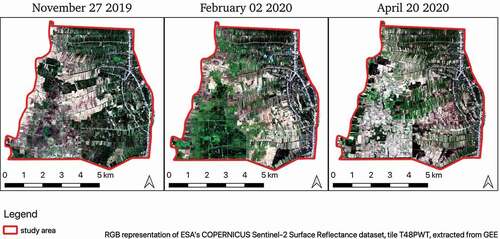
Overall, six broad land use classes are defined: open water surfaces, bare/fallow land, urban/village areas, fruit trees, rice fields, and vegetable fields. Out of these, urban areas – located along the main road that runs in parallel with the river – and fruit trees are relatively static over the course of a year (neglecting urban spread and the planting or cutting down of trees). The other classes are highly dynamic. During the wet season, large swaths of low-lying land in the west and southwest of the area are inundated. Subsequently, these areas see one or two cycles of rice cultivation, before lying fallow for part of the year. The higher terrain in the east of the study area sees a complex mosaic of fields lying fallow and being cultivated. Figure 2 shows an RGB overview of the LULC dynamics in the study area during the dry season.

Figure 1. Location of the study area on the floodplains of the Cambodian Mekong Delta

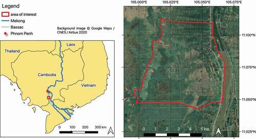
Figure 2. Landcover dynamics in the study area during the dry season, RGB image

Data used

The data used in this study stems from three sources: imagery from the Sentinel-1 and 2 satellites maintained by the European Space Agency (ESA), high-resolution SPOT-6 and 7 imagery, and fieldwork in Cambodia. For classifier training, images from three points in time in November 2019, February 2020, and April 2020 were used. At all three times, both Sentinel-1 and 2 data are available on either the same or adjacent dates. These dates fall at the beginning, middle, and end of the dry season, and account for the main changes in cultivation practices and LULC dynamics (cf. Figure 2). The SPOT-6 and 7 images and the fieldwork data are used for parameter tuning, calibration, and validation. Details on the satellite images used are given in Table 1.

Figure 3. Temporal distribution of training images and image time series used in this analysis, throughout the wet and dry season in the study area

Table 1. Overview of images used for training the classifiers. (* Resampled to 10 m across all bands during pre-processing.)

Satellite	Date	Sensor Characteristics	Resolution [m]
Sentinel-2A	27/11/2019	optical MSI	10–60*
Sentinel-2A	27/11/2019	optical MSI	10–60*
Sentinel-2A	05/02/2020	optical MSI	10–60*
Sentinel-2A	05/02/2020	optical MSI	10–60*
Sentinel-2B	20/04/2020	optical MSI	10–60*
Sentinel-2B	20/04/2020	optical MSI	10–60*
Sentinel-1A	26/11/2019	SAR	10
Sentinel-1B	27/11/2019	SAR	10
Sentinel-1A	31/01/2020	SAR	10
Sentinel-1B	01/02/2020	SAR	10
Sentinel-1A	18/04/2020	SAR	10
Sentinel-1B	19/04/2020	SAR	10
SPOT-7	29/11/2019	optical RGB	1.5
SPOT-7	29/11/2019	optical panchromatic	1.5
SPOT-6	02/02/2020	optical RGB	1.5
SPOT-6	02/02/2020	optical panchromatic	1.5
SPOT-6	20/04/2020	optical RGB	1.5
SPOT-7	26/04/2020	optical panchromatic	1.5

Sentinel-1

The ESA’s Sentinel-1 constellation consists of two satellites, Sentinel-1A and Sentinel-1B, which were launched in 2014 and 2016, respectively. Both satellites have a return period of 12 days, resulting in a combined Sentinel-1 overpass frequency of 6 days. They collect C-band synthetic aperture radar imagery in a variety of polarizations, instrument modes, and resolutions. For this study, interferometric wide swath (IW) images in the form of co-polarized VV and cross-polarized VH bands at 10 m resolution are used, as the most widespread type of imagery for LULC approaches using SAR (Khan et al., 2020; Ranjan & Parida, 2019; Tavares et al., 2019).

In total, six Sentinel-1A and B images taken in descending orbits are used to train and validate the classifiers for three different dates. The study area is located at an intersection area of two Sentinel-1 tiles. To reduce random speckle noise, mean composites of Sentinel-1 images taken on subsequent days are created for each of the training points in time (cf. Table 1). To test the trained classifier and create a LULC time series, 117 SAR images between 01/11/2019 and 31/10/2020 are used. As can be seen in Figure 3, these images are distributed regularly throughout the year.

Sentinel-2

Like Sentinel-1, the ESA’s Sentinel-2 collection consists of a pair of satellites. Sentinel-2A was launched in 2015, followed by Sentinel-2B in 2017. Both satellites have a return period of 10 days, resulting in a combined Sentinel-2 image frequency of 5 days. The constellation provides multi-spectral optical imagery for a total of 12 spectral bands ranging from the blue to the short wave infrared spectrum.

Like for Sentinel-1, overlapping Sentinel-2 tiles are available in the study area. To train the classifiers, three composites of six cloud-free optical images are used (cf. Table 1). For the land use time series classification, 47 images between 01/11/2019 and 31/10/2020 are used. However, it must be noted that these images are not distributed regularly across the year. As shown in Figure 3, multiple images are available for every month during the dry season. During the wet season, when cloud cover is high, this is not the case.

Data for calibration and validation

This study uses SPOT-6 and 7 images to generate training points for the classification algorithms. SPOT (Satellite Pour l’Observation de la Terre) is a high-resolution satellite operated commercially by Spot Image. It provides panchromatic and multi-spectral images at 1.5–6 m resolution. Complemented by knowledge of the general LULC distribution patterns in the study area, points are set manually where land use classes are discernible with reasonable certainty on the high-resolution images. Overall, 9,000 training points are set – 1500 per training class (cf. Table 2). While this procedure yields an extensive set of training data, it also introduces some class noise. This describes training points that carry erroneous labels, which can impact the quality of the classification. However, it is still salient to harness a dataset generated in this way for comparative purposes, as noise is a common problem in supervised remote sensing approaches (Frenay & Verleysen, 2014; Pelletier et al., 2017).

Table 2. Distribution of training data points across the multi-temporal images

Category	Point Nr. Fieldwork Set			Point Nr. Extended Set
	Nov.	Feb.	Apr.	Nov.	Feb.	Apr.
Open water surfaces	100	11	10	500	500	500
Bare/fallow land	120	120	120	500	500	500
Urban/village areas	120	120	120	500	500	500
Fruit trees	120	120	120	500	500	500
Rice fields	120	120	100	500	500	500
Vegetable fields	50	100	21	500	500	500

A final component of the data setup of this paper is ground-truth training data collected at the study site in autumn 2019 and spring 2020. In total, 1,712 training points were collected. The majority were set on site using a manual GPS device (horizontal accuracy: 10 m). In addition, some were set manually using geo-referenced in-situ images from an unmanned aerial vehicle (UAV). However, unlike for the training data derived from SPOT-6 and 7 images, the training points from the field surveys are not distributed equally between classes. For example, while the November fieldwork training set includes 630 points, its April equivalent only contains 491 (cf. Table 2). While this training sample is smaller and its points are unevenly distributed between classes and dates, the confidence of its label attribution is considerably higher.

Methodology

A general outline of the classification workflow is given in Figure 4. Following pre-processing, nine datasets are generated on which the classifiers are tested. These datasets derive from the use of different imagery types alone and in combination, as well as different band sets (see Table 3). Parameter tuning, calibration, and validation are performed for each of the nine datasets separately, using both the limited training points derived from fieldwork, and the extended training points generated on the basis of the SPOT-6 and 7 images, resulting in 18 different configurations of input data for each of the four classifiers. Finally, the best-performing algorithm is chosen and applied to the optical, radar, and combined dataset to generate a LULC classification spanning the entire period between 01/11/2019 and 31/10/2020.

Figure 4. Classification workflow

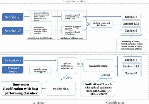
Table 3. Overview of image datasets used

Dataset Nr.	Imagery	Band Set
1	Sentinel-1	Full
2	Sentinel-1	Reduced
3	Sentinel-1	Minimal
4	Sentinel-2	Full
5	Sentinel-2	Reduced
6	Sentinel-2	Minimal
7	Sentinel-1 & 2	Full
8	Sentinel-1 & 2	Reduced
9	Sentinel-1 & 2	Minimal

Image pre-processing

To a certain degree, both Sentinel-1 and 2 images are already provided in pre-processed form in GEE.

Sentinel-1 images undergo pre-processing during ingestion in GEE based on the ESA’s Sentinel-1 toolbox. In this process, metadata is updated with a restituted orbit file, border noise and thermal noise are removed, and radiometric calibration and orthorectification are applied. The fact that images are provided in pre-processed form in GEE’s JavaScript API removes one of the main hurdles many researchers face in using SAR data. In fact, several studies have used GEE as a source of SAR images, even though their analyses were subsequently conducted in different environments (Amani et al., 2020; Tamiminia et al., 2020).

As a basis for classification, additional bands are generated for SAR imagery using the original VV and VH bands (cf. Table B2). Three of these are based on arithmetic operations (VV/VH, VV-VH, (VV+VH)/2) which previous studies found to yield increased accuracies for LULC approaches (Slagter et al., 2020). The others are based on a classic Grey Level Co-occurrence Matrix (GLCM), encompassing Haralick texture features (Haralick et al., 1973). These features describe image texture through interpretable descriptors and have been found to add valuable information for LULC analyses (Clerici et al., 2017; Lin et al., 2020; Mishra et al., 2019). Texture features are calculated separately for both the VV and VH polarization, parameterized with a 5 × 5 window size. Following previous studies (Nizalapur & Vyas, 2020), angular second moment (ASM), contrast (CONTRAST), correlation (CORR), inverse difference moment (IDM), entropy (ENT), dissimilarity (DISS), and variance (VAR) are used as added bands for classification in this study. Following the calculation of the texture features, a refined Lee speckle filter (Yommy et al., 2015) is applied to smooth the original VV and VH bands in order to reduce speckle, since not all data datasets use the generated texture bands.

Sentinel-2 images are available in pre-processed form in GEE. The sen2cor algorithm (Main-Knorn et al., 2017) has been applied to transform Top of the Atmosphere (TOA) reflectance to surface reflectance (BOA). For this analysis, all bands are automatically resampled to 10 m resolution by the GEE processing algorithm. For the time series calculation, a cloudy pixel threshold of <20% is introduced, and the remaining clouds are masked using a simple bit-mask based on the QA band.

Additional spectral indices (cf. Table 4) are calculated on the basis of native bands (cf. Table B1) to generate ancillary layers of information that serve as input for the classification algorithms, which past studies have found to be valuable in increasing classification accuracies (Godinho et al., 2016). These are based on a range of bands employed in past studies for various LULC analyses using different classification algorithms (Ouattara et al., 2020).

Table 4. Spectral indices calculated for optical Sentinel-2 imagery

Index	Calculation	Reference
Enhanced vegetation index	$EVI=2.5\ast \left(NIR-Red\right)/\left(NIR+6\ast Red-7.5\ast Blue\right)$	Huete et al. (2002)
Two-band enhanced vegetation index	$EVI2=2.5\ast \left(NIR-Red\right)/\left(NIR+Red\right).$	Jiang et al. (2008)
Green normalised difference vegetation index	$GNDVI=\left(NIR-Red\right)/\left(NIR+Red\right)$	Gitelson et al., 1996
Modified normalised difference water index	$MNDWI=\left(Green-SWIR2\right)/\left(Green+SWIR\right)$	Xu (2006)
Modified soil adjusted vegetation index	$MSAVI=NIR+0.5-(0.5\ast \sqrt{\left({\left(2\ast NIR+1\right)}^2\right)}-8\ast \left(NIR-\left(2\ast Red\right)\right)$	Qi et al., 1994
Normalised difference red edge index	$NDRE=\left(NIR-RE\right)/\left(NIR+RE\right)$	Gitelson and Merzlyak (1996)
Normalised difference moisture index	$NDMI=\left(NIR-SWIR\right)/\left(NIR+SWIR\right)$	Wilson and Sader (2002)
Normalised difference built-up index	$NDBI=\left(SWIR-NIR\right)/\left(SWIR+NIR\right)$	Zha et al. (2003)
Normalised difference vegetation index	$NDVI=\left(NIR-Red\right)/\left(NIR+Red\right)$	Rouse et al. (1974)
Normalised difference water index	$NDWI=\left(Green-NIR\right)/\left(Green+NIR\right)$	McFeeters (1996)
Normalised difference water index 2	$NDWI2=\left(NIR-SWIR2\right)/\left(NIR+SWIR2\right)$	Gao (1996)
Normalised ratio vegetation index	$NRVI=\left(Red/NIR-1\right)/\left(Red/NIR+1\right)$	Baret and Guyot (1991)
Ratio vegetation index	$RVI=Red/NIR$	Jordan (1969)
Soil-adjusted vegetation index	$SAVI=\left(NIR-Red\right)/\left(NIR+Red+1\right)+2$	Huete (1988)
Specific leaf-area vegetation index	$SLAVI=NIR/\left(Red+SWIR2\right)$	Lymburner et al. (2000)
Simple ratio vegetation index	$SRVI=NIR/Red$	Birth and McVey (1968)

Creation of image datasets

In total, parameter tuning, calibration, and validation are performed on nine image datasets (cf. Table 3).

First, three main sets of images are created – one containing only SAR imagery, one containing optical imagery, and one in which combined images are created by stacking all available optical and SAR bands into a single image. Then, each of the three imagery sets is further subdivided into three tiers depending on how many bands are used for classification (see Table 5). One tier includes a band set that encompasses all native bands, spectral indices, and texture features. A reduced band set includes the native image bands as well as some additional indices. Finally, a minimal set consists only of the VV and VH bands for SAR, and the RGB bands for optical imagery.

Table 5. Band sets of spectral indices and texture features. For the combined imagery set, these bands are stacked

Band Set	SAR Imagery	Optical Imagery
Full Set	VV, VH, VV/VH, VV-VH, (VV+VH)/2, ASM, CONTRAST, CORR, DISS, IDM, ENT, VAR	R, G, B, RE2, RE3, NIR, RE4, SWIR1, SWIR2, NDVI, NDBI, NDWI, MNDWI, MSAVI, GNDVI, NDRE, NDWI2, EVI, EVI2, NRVI, RVI, SAVI, SLAVI, SRVI
Reduced Set	VV, VH, VV/VH, VV-VH, (VV+VH)/2,	R, G, B, RE2, RE3, NIR, RE4, SWIR1, SWIR2, NDVI, SAVI
Minimal Set	VV, VH	R,G,B

Parameter tuning and classification

Each dataset is calibrated with 80% and validated with 20% of both the fieldwork and the SPOT-based training data, for each of the four classifiers. Preceding calibration, each classifier undergoes parameter tuning. A short description of each classifier as well as the associated tuning parameters is given below.

Naïve Bayes (NB)

This classifier relies on a simple probabilistic approach that is based on the Bayes theorem (John & Langley, 1995). It is referred to as naïve because it relies on the assumption of conditional independence between every pair of features, and a Gaussian probability distribution (Zhang, 2005). In reality, this condition is frequently not met, particularly in more complex situations and datasets. Nonetheless, several studies have found the simplistic approach to yield satisfying results (Diengdoh et al., 2020; Johnson & Iizuka, 2016), particularly in cases where only a limited number of input features is available. This may be due to the fact that, in general, even a small training set is sufficient to minimize the average risk of the classification error and compute the decision surface. Some studies have also argued that dependence distribution among classes could account for the surprisingly good performance of NB (Kuncheva, 2006). In GEE’s implementation of NB, the only parameter that needs to be tuned for performance is the smoothing factor λ.

Classification And Regression Trees (CART)

CART classifiers belong to the family of decision tree (DT) classifiers. The basic approach of this type of classifier is to find the attribute or threshold that splits a training dataset most effectively into subsets. This split then becomes a node in the tree, with the two subsets forming branches. Each subset is then split into further subsets until only a non-splitable end node (also known as a “leaf node”) remains. The main criterion in performing every split is the normalized information gain (Shalev-Shwartz & Ben-David, 2014). Once grown using the training dataset, the decision tree can then be applied to new samples. A considerable disadvantage of this approach is its high sensitivity to the training dataset. Even globally negligible modifications in the training data can lead to fundamentally different tree structures (Shelestov et al., 2017). To improve classifier performance, the number of leaf nodes in each tree (maxNodes) is tuned.

Random Forest (RF)

Random Forest (RF) is a recursive partitioning technique that is based on the construction of an ensemble of classification and regression trees (hence the term forest). Each tree is trained using the same method as described above for CART. However, to increase computational efficiency, each tree only utilizes a random subset of features at each node – this step also reduces correlation (and accounts for the second element in the nomenclature of the classifier). Trees are bundled together computationally through bootstrap aggregating (“bagging”) (Breiman, 1996). The final classification result for a new sample is then obtained through a majority vote of individual tree results. Overall, this approach is less sensitive to overfitting and noisy data, two of the most considerable pitfalls of CART approaches (Breiman, 2001). For RF tuning, the number of trees (nTree) and the number of variables per split (mTry) have to be optimized. Past studies found that satisfactory, stable results could be produced with a number of trees ranging between 200 and 500 (Belgiu & Dragut, 2016). To find the optimal RF model, this study tested nTree = [50:750] with a step size of 50, and mTry = [1:15] with a step size of 1.

Gradient Tree Boosting (GTB)

Like RF, Gradient Tree Boosting (GTB) algorithms utilize an ensemble of decision trees. However, its basic approach differs in that it limits the complexity of trees, confining each individual tree to a weak prediction model. It achieves classification accuracy by iteratively combining an ensemble of these weak learners into strong ones by minimizing a differentiable loss function at every step, following a gradient descent procedure (Friedman, 2002). To reduce correlation between trees, each new tree is constructed on the basis of a stochastically selected subset of training data. Recent studies have shown GTB algorithms, such as XGboost (Chen & Guestrin, 2016) to outperform classifiers such as SVM, RF, and KNN (Godinho et al., 2016), especially on unbalanced datasets. However, GTB are often prone to overfitting, a risk that can be minimized through parameter tuning.

In terms of parameters to be adjusted, the number of trees (nTree) is varied between 50 and 200, with a step size of 10. Furthermore, GTB requires a parameter to be specified to determine how many nodes a decision tree in the ensemble can have. Since GTB is based on weak learners, the maxNodes parameter is typically low, with a range of [2:10] with a step size of 1 being tested in this study. In addition, the sampling rate for stochastic gradient tree boosting, and the shrinkage rate, which controls the learning rate of the algorithm, need to be optimized. In this study, a range of [0.45:0.75] with a step size of 0.05 was tested for the former, and [0.005, 0.01, 0.05, 0.1, 0.25, 0.5] for the latter. Finally, all three loss functions available in GEE for GTB were compared – least squares, least absolute deviation, and Huber. It must be noted that recommendations for nTree tuning usually include larger numbers of tree. Elith et al., (2008), for example, recommend nTree = 1000 for tuning as a rule of thumb. However, the GEE implementation of GTB currently produces an error when more than 200 trees are employed for the data configuration in this study. This may be due to the fact that GTB was only recently implemented in GEE by the developers’ team and will be further discussed below.

Support Vector Machines (SVM)

The founding principle of this approach is to find the boundary that maximizes the distance from the nearest data point of all classes (Noble, 2006). These points are used for the construction of support vectors, which, in turn, form the basis for the computation of the maximum-margin hyperplane that serves as a boundary. The dimensionality of this hyperplane is determined by the number of features to be used for classification. For non-linear data, a kernel is applied to transform low-dimensional data to make it separable via the SVM approach in a higher-dimensional sphere (Cortes & Vapnik, 1995). Frequently used kernels include linear, Gaussian Radial Basis Function (RBF), sigmoid, and polynomial kernels (Amari & Wu, 1999). The main advantage of SVM is its high potential for generalization.

In terms of tuning SVMs, the first choice to make is to pick a kernel. For LULC approaches, RBF and Linear kernels are frequently used (Kavzoglu & Colkesen, 2009; Shi & Yang, 2015). Then, the cost parameter C needs to be optimized, as well as the γ value in case the RBF kernel is used. The γ value determines the RBF kernel width and thus affects the smoothing of the hyperplane which divides classes. The C parameter sets the threshold for permitted misclassification of non-separable training data (Thanh Noi & Kappas, 2017). If it is too large, it can lead to over-fitting (Ghosh & Joshi, 2014). This study follows (Li et al., 2014) in using 10 C values (2^[−2:7]) as well as 10 γ values (2^[−5:4]) for parameter tuning.

Validation and statistical analysis

Finally, the classification results of each algorithm using each combination of imagery, band set, and training data are validated. For this, the remaining randomly selected 20% of the field work and SPOT-based datasets are used. Overall accuracy as well as producer and consumer accuracies is calculated (Congalton, 1991). To ascertain whether the choice of input imagery, training data, and band set has statistically significant impacts on classifier performance, the non-parametric Kruskal Wallis test (Kruskal & Wallis, 1952) is used.

Results

Optimal tuning parameters

The tuning parameters that yielded the highest accuracies for each classifier and each of the nine image subsets, and that are used in the remaining of the analysis, are given in Table 6. The full set of tuning parameters and their associated accuracies are given in the supplementary materials. The results show that the parameter values yielding the highest accuracies varied considerably for RF (nTree and mTry) and for SVM (C and γ). For RF, the nTree used for the final analysis varies between 50 and 600, and nTry ranges from 1 to 14. For SVM, optimal classification accuracy is achieved using C values that vary along the full tuning spectrum. Similarly, the optimal γ value for the RBF kernel ranges from 2⁻⁵ to 2⁴ . There are no discernible trends along the lines of imagery type, band sets, or training datasets.

Table 6. Tuning parameters for optimal accuracies for each classifier and band set

Image Source			Sentinel-1			Sentinel-2			Sentinel-1 & 2
Band Set	Classifier	Parameter	All bands	Restricted	Minimum	All bands	Restricted	Minimum	All bands	Restricted	Minimum
Fieldwork training set	NB	λ	-	-	-	-	-	-	1E-10	-	-
	CART	maxNodes	6	6	5	6	6	5	6	6	5
	RF	nTree	100	600	150	250	200	250	350	400	500
		mTry	14	4	2	14	4	2	3	1	2
	GTB	nTree	180	170	170	190	130	50	80	160	190
		maxNodes	7	3	10	10	10	10	6	8	9
		shrinkage	0.01	0.05	0.1	0.01	0.05	0.1	0.25	0.1	0.05
		samplingRate	0.7	0.7	0.75	0.65	0.7	0.7	0.6	0.7	0.65
		loss function	-	-	-	-	-	-	-	-	-
	SVM	C (linear)	16	1	0.5	0.25	0.25	0.25	16	1	8
		C (RBF)	128	1	16	128	128	128	-	-	2
		γ	0.03	-	0.03	16	16	16	0.03	0.06	0.03
SPOT training set	NB	λ	1E-10	-	-	-	-	-	1E-10	-	-
	CART	maxNodes	6	6	6	6	5	5	6	6	6
	RF	nTree	400	450	400	550	50	500	400	450	400
		mTry	8	4	2	11	1	1	8	4	2
	GTB	nTree	200	190	200	180	190	190	160	190	180
		maxNodes	10	9	10	9	10	9	10	10	9
		shrinkage	0.1	0.25	0.1	0.25	0.05	0.05	0.1	0.25	0.05
		samplingRate	0.7	0.75	0.75	0.75	0.65	0.75	0.75	0.7	0.65
		loss function	-	-	-	-	-	-	-	-	-
	SVM	C (linear)	0.25	0.25	0.25	128	128	64	0.25	0.25	0.25
		C (RBF)	2	2	16	64	64	64	2	2	16
		γ	0.03	-	0.03	16	16	16	0.03	-	0.03

In contrast to this, the optimal values for the tuning parameter λ for NB and CART’s maxNodes vary little. In the case of λ, most combinations of imagery, band sets, and training data show little sensitivity to value tuning. Where differences in accuracies depending on λ are observable, the highest accuracies can be reached with λ = 1*10⁻¹⁰. For maxNodes, the CART classifier globally reaches its highest accuracies using either 5 or 6 nodes.

As for GTB, parameter tuning revealed low sensitivities for some parameters, and higher discrepancies in accuracies for others. The type of loss function employed, for example, has a virtually untraceable effect on accuracies. The shrinkage function, on the other hand, showed optimal values between 0.01 and 0.25, and the sampling rate between 0.6 and 0.75. For nTree and maxNodes there was a noticeably larger variation for optimal parameter values for the fieldwork training set than for the extended training set. In the former, values for nTree ranged between 50 and 190 and for maxNodes between 3 and 10. In the latter, the optimal value for nTree lay between 160 and 200, and for maxNodes between 9 and 10.

Overall accuracy

The maximum overall accuracies achieved by each classifier depending on imagery type, band set, and training data, are given in Table 7. Accuracies over 85%, which previous studies have deemed satisfactory for LULC purposes (Denize et al., 2018; Khan et al., 2020; Steinhausen et al., 2018) are highlighted in bold.

Table 7. Comparison of overall accuracies (OA) by classifier, imagery type, training set, and band set. OA values of over 85 are marked in bold

			Overall Accuracy [%]
Imagery	Training Set	Band Set	NB	CART	RF	GTB	SVM RBF	SVM Linear
Optical	Fieldwork	Full	35	70	75	72	63	66
		Reduced	46	70	76	75	58	69
		Minimal	49	63	70	67	58	53
	Extended	Full	32	71	85	85	60	75
		Reduced	63	75	86	85	61	75
		Minimal	53	60	75	72	61	60
SAR	Fieldwork	Full	42	59	61	53	55	54
		Reduced	23	66	67	55	52	52
		Minimal	21	55	64	66	51	50
	Extended	Full	9	55	61	69	57	56
		Reduced	1	54	75	71	56	55
		Minimal	1	54	74	65	55	52
Combined	Fieldwork	Full	48	88	92	93	21	88
		Reduced	72	88	91	92	19	90
		Minimal	60	81	85	87	24	73
	Extended	Full	53	81	93	94	32	86
		Reduced	69	82	93	94	32	92
		Minimal	49	66	85	87	46	79

The results show that GTB globally reaches the highest overall accuracy, at 94%. This value is reached using combined imagery, the extended dataset derived from SPOT imagery, and both the full and the reduced band set. RF also yields similarly high values (93%) using the same combination of imagery, training dataset and bands. For the fieldwork dataset, the highest accuracies are also reached by GTB and RF. GTB yields an overall accuracy of 93% for the full and 92% for the reduced band sets using combined optical and SAR imagery. For the same input configuration, RF yields accuracies of 92% and 91%, respectively. Furthermore, GTB and RF also reach accuracies of over 85% using all other combinations of bands and training sets for the combination of Sentinel-1 and 2 imagery, and for the use of the extended training set and the full and reduced band sets for optical-only imagery.

SVM using a linear kernel and combined optical and SAR imagery is third in terms of overall accuracy. Accuracies of up to 92% are achieved using the extended training dataset and the reduced band set. Like RF, SVM also yields high accuracies when trained using the fieldwork dataset and the reduced band set. It furthermore attains accuracies of 88% and 86%, respectively, for the use of the full band set and both training data sets. For the variation of SVM using an RBF kernel, the overall classification accuracy does not surpass 63%.

The CART classifier reaches overall accuracies of up to 88%, when trained using combined imagery, the fieldwork dataset and either the full or reduced band sets. Far below this mark is the Naive Bayes classifier. Its highest overall accuracies, at 72%, is reached using the combined optical and SAR imagery.

SAR- and optical-only vs. combined imagery

Overall, the results show a marked increase in accuracy for the majority of classifiers when combined imagery is used, as opposed to SAR and optical-only imagery. For RF, optical-only imagery leads to an average accuracy of 78% across training and band sets, for GTB to 76%. For SAR-only imagery, this average lies at only 67% and 63%, respectively. The combination of both imagery types, however, yields an average accuracy of 90% for RF, and of 91% for GTB. Similarly, the CART, SVM, and NB classifiers also yield their best accuracies using the combined imagery.

As illustrated in Figure 5, the combined imagery yields considerably higher accuracies for NB, CART, RF, GTB, and SVM using a linear kernel than optical or SAR images alone. For CART, RF, and GTB the improvement in accuracy when using combined imagery in comparison to optical-only imagery is statistically significant (p < 0.05). In addition, the CART classifier using optical imagery shows considerable variability with respect to accuracies. The improvement in comparison to using SAR-imagery only is statistically significant for NB, CART, RF, and SVM using a linear kernel. However, for SVM using an RBF kernel, the reverse is true – the combined imagery yields considerably lower accuracy values than either optical- or SAR-only imagery.

Figure 5. Box plot of overall accuracies by imagery used and classifier, and significance of variation of accuracies depending on imagery type used

Choice of training data and band sets

In general, the extended training data yields the highest overall accuracies for GTB, RF and SVM using both a linear and RBF kernel. For CART and NB, however, the training set based on fieldwork data leads to higher accuracies. GTB, RF and SVM using a linear kernel also yield accuracies of over 85% using the fieldwork dataset (cf. Table 7 and supplementary materials). It can be noted that the use of the extended data set leads to a higher accuracy improvement in optical and SAR-only imagery than in the combined imagery. For example, for RF applied to optical imagery, the average overall accuracy achieved using the fieldwork dataset lies at 74%, whereas the extended dataset yields an average overall accuracy of 82%. In contrast, for combined imagery the average RF using fieldwork training data lies at 89%. Using the extended dataset only increases this average overall accuracy to 90%.

As for the band set, it emerges that the extended and fieldwork datasets produce comparable accuracies for CART, RF, and GTB. SVM using a linear kernel, however, produces distinctly higher accuracies on the basis of the reduced band set. Furthermore, SVM using the RBF kernel produces its highest overall accuracies when the minimal band set is used.

Accuracy by class

The accuracy with which each land cover class is classified by each algorithm varies considerably. Consequently, this impacts the overall classification accuracy at different points in the time series of images between 01/11/2019 and 31/10/2020, when the classes have a different predominance.

Water, for example, has a relatively high consumer and producer accuracy (cf. Table 8). While NB tends to errors of omission, mis-classifying water as urban areas, the other classifiers succeed in delineating surface water regions with fairly high confidence. RF and GTB in particular delineate water well, with producer accuracies of 98% and 97%, and consumer accuracies of 97% and 98%, respectively, followed by SVM (97% and 96%, respectively). Consequently, inundated areas, as they can be observed in November, are represented well.

Table 8. Producer and consumer accuracies for NB, CART, RF, GTB and SVM using a linear kernel. SVM (RBF) is not included due to low accuracies

	Producer Accuracy						Consumer Accuracy
Classifier	Water	Urban	Fallow	Fruit	Rice	Veg.	Water	Urban	Fallow	Fruit	Rice	Veg.
NB	86	75	89	40	83	58	100	79	79	84	64	39
CART	89	91	94	91	87	59	85	91	96	89	88	59
RF	98	96	95	95	85	79	97	96	97	93	91	81
GTB	97	98	97	97	79	82	98	96	98	94	92	80
SVM (Linear)	97	96	93	97	72	66	96	97	99	87	88	79

In contrast, the classifiers exhibit greater difficulties in separating bare/fallow land from urban areas, and vegetable fields from rice paddies. While CART, RF, GTB, and SVM succeed well in classifying the permanent urban areas in the east of the study area, they also tend to misclassify fields lying fallow during the dry season as urban areas. The discrepancy between the size of the areas classified as fallow across the year depending on which classifier is used is also shown in Figure 7. In terms of consumer accuracy, SVM using a linear kernel can boast the best performance in delineating urban and fallow land. In contrast, RF and GTB exhibit a better performance in separating rice paddies and vegetable plots, both in terms of producer and consumer accuracies.

Figure 6. Comparison of classification results using the best-performing configuration of NB, CART, RF, GTB, and SVM (linear)

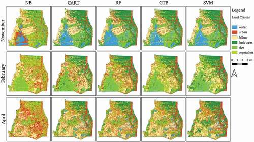
Figure 7. Time series of areas classified as bare/fallow using the training point set based on SPOT-images and CART, RF, GTB, and SVM (linear) between October 2019 and September 2020. NB and SVM (RBF) are not included due to low accuracies

Discussion

Benefits of combining imagery

Most saliently, this study highlights the multiple benefits of combining Sentinel-1 and 2 imagery for various classifiers. For all classifiers except SVM using an RBF kernel, combined imagery yields the highest classification accuracy. Especially for SVM using a linear kernel, the combination of optical and SAR imagery brings a relative increase in overall classification performance. This is in line with several studies that have found marked benefits in adding information from radar images to optical ones for LULC classification (Denize et al., 2018; Van Tricht et al., 2018). What is notable in the present study is the consistent and considerable increase in accuracy that results from the combination of image sources. Tavares et al. (2019), for example, note a rise in accuracy from 89% using Sentinel-2 only to 91% using combined imagery. Similarly small accuracy improvements were reported by (Lu et al., 2018). In contrast, the present study finds increases in accuracy of up to 15 percentage points. In addition, it can be noted that the combination of imagery also leads to a reduction of the impact of the training dataset. It can be conjectured that this is due to the fact that additional layers of information counter-balance the noise in training data and make it more easily separable for classifiers.

Configuring input parameters and data for optimal results

Broadly, the results of the analysis illustrate the wide variations in the values of optimal parameters leading to the best classification accuracies for RF, GTB, and SVM, as well as the considerable impact of the choice of kernel for SVM. Regarding the RF parameter of nTree, for example, previous studies (e.g., Thanh Noi & Kappas, 2017) found that accuracies tended to increase with a rising number of classification trees in each random forest, and that further increasing the number of trees led to stability in the accuracy of the results, starting at ca. 250 trees. Others also note that forests with a larger number of trees do not necessarily perform better than those with fewer (Oshiro et al., 2012). The present analysis shows that optimal accuracy values for some data configurations can be reached at nTree = 50 already, and that increasing the number of trees can lead to a noticeable decrease in accuracy. This underscores the importance of performing parameter tuning prior to applying each of these classifiers in a new setting, with varying input data configurations. As the tuning results for GTB show, the importance of parameter tuning is also dependent on the quality of the training dataset. While optimal parameter values for nTree and maxNodes vary little for the extended training set, greater discrepancies in values needed to achieve optimal overall classification accuracies are observed using the fieldwork-based training dataset.

Broadly, in terms of band sets and training data, this analysis illustrates the nuanced balance between adding additional layers of information through texture features and spectral indices, and introducing noise that can detract from classification accuracies. Most prominently, it emerges that it isn’t necessarily the set of bands with the highest number of additional indices and texture features that yields the highest accuracies. Nor is it the minimalist approach taking as a basis of classification only the bare minimum of raw bands. Rather, it is the set of curated raw bands and spectral indices, as well as bands arithmetically calculated from the SAR imagery’s VV and VH bands, that leads to the best classification performance. Most probably, this is due to the fact that any additional information offered by certain spectral indices is drowned out by the noise that other, less meaningful, indices produce. This result underlines findings from previous studies, such as Da Silva et al. (2020), which concluded that the NDVI, EVI, and SAVI offer the highest additional values for LULC approaches.

Overall classifier performance

When it comes to comparing algorithms in terms of accuracy, this analysis shows that the GTB and RF classifiers consistently exhibit the best performance under a number of different input data configurations, with GTB slightly exceeding RF in terms of accuracy. It must be highlighted that GTB achieves this performance despite the fact nTree is currently limited to less than 200. Though SVM shows similarly high classification accuracies for combined imagery and the use of a reduced band set, GTB and RF performance is consistently superior with regard to all constellations of input data – imagery type, training dataset, and band set. It is only in certain land cover classes – such as the separation of urban areas and bare land – that SVM outperforms RF and GTB. Several previous studies have debated the compared performance of RF and SVM. Ma et al. (2018) found RF to be generally superior in a review of object-based LULC classification approaches, as did Talukdar et al. (2020) in a comparison of machine learning approaches for LULC classification. Rana and Venkata Suryanarayana (2020) by contrast, found SVM performance to be superior, especially in combination with a principal component approach. In addition, several studies have also factored GTB into the comparison. For example, Georganos et al. (2018) found the XGboost implementation of GTB to systematically outperform RF and SVM, especially on the basis of an extended feature set. Overall, it appears that SVM performs well when studies aim to fine-tune parameters and investigate specific applications, whereas RF and GTB offer more solid, generalizable applications for LULC approaches, and a lower sensitivity to various input data. This higher sensitivity of SVM to the types of input imagery and the training data set is in line with findings from earlier studies. Pelletier et al. (2017), for example, compared the effect of training data noise on supervised LULC classification using SVM and RF. The results found RF to be significantly more robust towards both random and systematic noise of training labels.

As for the other classifiers available in GEE that were tested in this study, it emerges that NB is ill-suited for LULC applications, with low overall accuracies. CART, on the other hand, yields solid results for the combined imagery type. In particular, it can be noted that this classifier performs better when trained using only the fieldwork data. It can be conjectured that this may be due to the more precise nature of the points in this training data set. Even though there are fewer overall than in the extended dataset, and they are unevenly distributed between classes, their label attribution carries a higher certainty. As mentioned above, a higher label noise is likely to have been introduced in the extended dataset derived from SPOT during its creation (Frenay & Verleysen, 2014). CART appears to be more sensitive to noise of this kind in the input data, which can be related to the fact that, unlike RF, it only relies on a single threshold to define a node to split data into subsets. In RF, where this process is repeated multiple times, noise can be balanced out more easily. The discrepancy in the classification for CART depending on the training point set is illustrated starkly by contrasting Figures 6 and 7, the former of which is generated with the configuration of input parameters yielding the highest accuracies (meaning the fieldwork training point set for CART), and the latter of which uses the extended dataset generated on the basis of SPOT images as input. In the former, the extents of bare land towards the end of the dry season are higher in the CART classification than in RF or SVM. In the latter, the reverse is true.

Conclusion

Overall, this study illustrates the considerable benefits of using a combination of optical and SAR imagery in supervised multi-temporal LULC classifications in Google Earth Engine. When using GTB, the accuracies of these classifications can reach up to 94%, despite some current limitations in the classifier configuration. The results of this study also reveal that combining Sentinel-1 and Sentinel-2 imagery improves overall classification accuracy by 10–15 percentage points in comparison to analyses based on optical-only imagery. Furthermore, the results of the analysis show that combining different sources of imagery reduces the impact of the size and quality of the training data set. They further highlight that out of all the classifiers available in Google Earth Engine, GTB yields the highest overall classification accuracies, performing best in a variety of combinations of input data, training points, and band sets.

In general, the use of the extended training data, with points set manually on the basis of high-resolution SPOT imagery, leads to higher accuracies, despite the higher label noise in comparison to the smaller fieldwork dataset. It can equally be concluded that a carefully selected set of native bands, spectral indices, and texture features used as a basis for classification results in equal or better classifier performance than either a minimalist set, or a large variety of additional bands, especially when using SVM. This underscores the delicate balance between adding indices and texture features as auxiliary layers of information for classification, and the noise that is introduced through their addition, which may impede classification accuracy. Finally, this study also highlights the importance of tuning various input parameters prior to classification, and of comparing basic classifier settings, such as the choice of SVM kernel.

Overall, this study showcases the considerable differences in the outputs of LULC analyses on the GEE cloud computing platform that can result from the choice of imagery, input bands, classifiers, and parametrization – which can lead to vast disparities when applied to larger areas. These results can provide preliminary guidance to researchers to improve the accuracy of LULC analyses, which provide essential inputs into studies ranging from agriculture to hydrology.

Acknowledgments

The authors thank the Equipex Geosud project and the Theia network for making the SPOT-6 & 7 images used in this study available free of charge for research purposes, the French Development Agency (AFD) for its support through the COSTEA project, and our colleagues at the Institute of Technology of Cambodia as well as the Royal University of Agriculture for their invaluable partnership and support of field work. We further thank the anonymous reviewers of this paper for their valuable insights and suggestions for improvements.

Data and code availability

All the code used to produce the analyses in this study is available in the GEE JavaScript environment: https://code.earthengine.google.com/?accept_repo=users/christinaannaorieschnig/New_LULC

Disclosure statement

No potentiial conflict of interest was reported by the author(s).

Appendix A. Table of Abbreviations

Table A1. Abbreviations used in the text.

Table

Acronym	Definition
ANN	Artificial Neural Networks
API	Advanced Programming Interface
ASM	Angular Second Moment
BOA	Bottom of the Atmosphere Reflectance
CART	Classification and Regression Trees
CNN	Convolutional Neural Networks
CORR	Correlation
DISS	Dissimilarity
DNN	Deep Neural Networks
DT	Decision Tree
ENT	Entropy
ESA	European Space Agency
EVI	Enhanced Vegetation Index
EVI2	Two-band Enhanced Vegetation Index
FCNN	Fully Convolutional Neural Networks
GBM	Gradient Boosting Methods
GEE	Google Earth Engine
GLCM	Grey Level Co-occurence Matrix
GNDVI	Green Normalised Difference Vegetation Index
GRD	Ground-Range Detected
IDM	Inverse Difference Moment
IW	Interferometric Wide Swath
KNN	K Nearest Neighbour
LULC	Land Use and Land Cover
LVQ	Learning Vector Quantization
MNDWI	Modified Normalised Difference Water Index
MSAVI	Modified Soil Adjusted Vegetation Index
NASA	National Aeronautics and Space Administration
NB	Naive Bayes
NDBI	Normalised Difference Built-up Index
NDMI	Normalised Difference Moisture Index
NDRE	Normalised Difference Red-Edge Index
NDVI	Normalised Difference Vegetation Index
NDWI	Normalised Difference Water Index
NDWI2	Normalised Difference Water Index 2
NRVI	Normalised Ratio Vegetation Index
OA	Overall Accuracy
RBF	Radial Basis Function
RF	Random Forest
RPART	Recursive Partitioning Regression Trees
RVI	Ratio Vegetation Index
S1	Sentinel-1
S2	Sentinel-2
SAVI	Soil-Adjusted Vegetation Index
SLAVI	Specific Leaf-Area Index
SPOT	Satellite Pour l’Observation de la Terre
SR	Surface Reflectance
SRVI	Simple Ratio Vegetation Index
SVM	Support Vector Machine
TOA	Top of the Atmosphere Reflectance
UAV	Unmanned Aerial Vehicle
VAR	Variance

Appendix B. Overview of Native Sentinel-1 and 2 Bands

Table B1. Sentinel-2 bands, their resolutions, and wavelengths.

Table

Sentinel-2 SR Band	Description	Native Resolution	Wavelength
B1	Aerosols	60 meters	443.9 nm (S2A)/442.3 nm (S2B)
B2	Blue	10 meters	496.6 nm (S2A)/492.1 nm (S2B)
B3	Green	10 meters	560 nm (S2A)/559 nm (S2B)
B4	Red	10 meters	664.5 nm (S2A)/665 nm (S2B)
B5	Red Edge 1 (RE1)	20 meters	703.9 nm (S2A)/703.8 nm (S2B)
B6	Red Edge 2 (RE2)	20 meters	740.2 nm (S2A)/739.1 nm (S2B)
B7	Red Edge 3 (RE3)	20 meters	782.5 nm (S2A)/779.7 nm (S2B)
B8	Near Infrared (NIR)	10 meters	835.1 nm (S2A)/833 nm (S2B)
B8A	Red Edge 4 (RE4)	20 meters	864.8 nm (S2A)/864 nm (S2B)
B9	Water vapor	60 meters	945 nm (S2A)/943.2 nm (S2B)
B11	Short-wave Infrared 1 (SWIR 1)	20 meters	1613.7 nm (S2A)/1610.4 nm (S2B)
B12	Short-wave Infrared (SWIR 2)	20 meters	2202.4 nm (S2A)/2185.7 nm (S2B)

Table B2. Sentinel-1 bands, their resolutions, and wavelengths

Table

Name	Resolution	Wavelenght	Description
HH	10 meters	5.405 GHz	Single co-polarization, horizontal transmit/horizontal receive
HV	10 meters	5.405 GHz	Dual-band cross-polarization, horizontal transmit/vertical receive
VV	10 meters	5.405 GHz	Single co-polarization, vertical transmit/vertical receive
VH	10 meters	5.405 GHz	Dual-band cross-polarization, vertical transmit/horizontal receive

References

- Abadi, M., Barham, P., Chen, J., Chen, Z., Davis, A., Dean, J., & Zheng, X. (2016). TensorFlow: A system for large-scale machine learning. In 12th {USENIX} Symposium on Operating Systems Design and Implementation ({OSDI} 16) (pp. 265–283). Savannah, GA: {USENIX} Association.
- Amani, M., Ghorbanian, A., Ahmadi, S. A., Kakooei, M., Moghimi, A., Mirmazloumi, S. M., Moghaddam, S.H.A., Mahdavi, S., Ghahremanloo, M., Parsian, S., Wu, Q, & Brisco, B. (2020). Google earth engine cloud computing platform for remote sensing big data applications: A comprehensive review. IEEE Journal of Selected Topics in Applied Earth Observations and Remote Sensing, 13(2020), 5326–5350. https://doi.org/https://doi.org/10.1109/JSTARS.2020.3021052
- Amari, S., & Wu, S. (1999). Improving support vector machine classifiers by modifying kernel functions. Neural Networks, 12(6), 783–789. https://doi.org/https://doi.org/10.1016/S0893-6080(99)00032-5
- Baret, F., & Guyot, G. (1991). Potentials and limits of vegetation indices for LAI and APAR assessment. Remote Sensing of Environment, 35(2–3), 161–173. https://doi.org/https://doi.org/10.1016/0034-4257(91)90009-U
- Belgiu, M., & Dragut, L. (2016). Random forest in remote sensing: A review of applications and future directions. ISPRS Journal of Photogrammetry and Remote Sensing, 114, 24–31. https://doi.org/https://doi.org/10.1016/j.isprsjprs.2016.01.011
- Birth, G. S., & McVey, G. R. (1968). Measuring the 1. Agronomy Journal, 60(6), 640–643. https://doi.org/https://doi.org/10.2134/agronj1968.00021962006000060016x
- Breiman, L. (1996). Bagging Predictors. Machine Learning, 24(2), 123–140. https://doi.org/https://doi.org/10.1007/BF00058655
- Breiman, L. (2001). Random Forests. Machine Learning, 45(1), 5–32. https://doi.org/https://doi.org/10.1023/A:1010933404324
- Carretero, J., & Blas, J. G. (2014). Introduction to cloud computing: Platforms and solutions. Cluster Computing, 17(4), 1225–1229. https://doi.org/https://doi.org/10.1007/s10586-014-0352-5
- Chen, T., & Guestrin, C. (2016). XGBoost. In Proceedings of the 22nd ACM SIGKDD international conference on knowledge discovery and data mining (pp. 785–794). New York, NY, USA: ACM. https://doi.org/https://doi.org/10.1145/2939672.2939785
- Clerici, N., Valbuena Calderón, C. A., & Posada, J. M. (2017). Fusion of Sentinel-1A and Sentinel-2A data for land cover mapping: A case study in the lower Magdalena region, Colombia. Journal of Maps, 13(2), 718–726. https://doi.org/https://doi.org/10.1080/17445647.2017.1372316
- Congalton, R. G. (1991). A Review of Assessing the Accuracy of Classifications of Remotely Sensed Data, 37(1). ftp://ftp.inpa.gov.br/pub/incoming/SIGLAB/Edwin/Curso_SIG_SR/SEPARATAS_RS-Amazonia/RemoteSensingEnvironment/congalton_1991.pdf
- Cortes, C., & Vapnik, V. (1995). Support-vector networks. Machine Learning, 20(3), 273–297. https://doi.org/https://doi.org/10.1007/BF00994018
- Crowley, M. A., Cardille, J. A., White, J. C., & Wulder, M. A. (2019). Multi-sensor, multi-scale, Bayesian data synthesis for mapping within-year wildfire progression. Remote Sensing Letters, 10(3), 302–311. https://doi.org/https://doi.org/10.1080/2150704X.2018.1536300
- Da Silva, V. S., Salami, G., Da Silva, M. I. O., Silva, E. A., Monteiro Junior, J. J., & Alba, E. (2020). Methodological evaluation of vegetation indexes in land use and land cover (LULC) classification. Geology, Ecology, and Landscapes, 4(2), 159–169. https://doi.org/https://doi.org/10.1080/24749508.2019.1608409
- Deines, J. M., Kendall, A. D., Crowley, M. A., Rapp, J., Cardille, J. A., & Hyndman, D. W. (2019). Mapping three decades of annual irrigation across the US high plains aquifer using Landsat and google earth engine. Remote Sensing of Environment, 233, 111400. https://doi.org/https://doi.org/10.1016/j.rse.2019.111400
- Denize, J., Hubert-Moy, L., Betbeder, J., Corgne, S., Baudry, J., & Pottier, E. (2018). Evaluation of using sentinel-1 and −2 time-series to identify winter land use in agricultural landscapes. Remote Sensing, 11(1), 37. https://doi.org/https://doi.org/10.3390/rs11010037
- Diengdoh, V. L., Ondei, S., Hunt, M., & Brook, B. W. (2020). A validated ensemble method for multinomial land-cover classification. Ecological Informatics, 56, 101065. https://doi.org/https://doi.org/10.1016/j.ecoinf.2020.101065
- Dinh, D. A., Elmahrad, B., Leinenkugel, P., & Newton, A. (2019). Time series of flood mapping in the Mekong Delta using high resolution satellite images. IOP Conference Series: Earth and Environmental Science, 266, 12011. Pan Pacific Hanoi, Vietnam. https://doi.org/https://doi.org/10.1088/1755-1315/266/1/012011
- Elith, J., Leathwick, J. R., & Hastie, T. (2008). A working guide to boosted regression trees. Journal of Animal Ecology, 77(4), 802–813. https://doi.org/https://doi.org/10.1111/j.1365-2656.2008.01390.x
- Foo, S. A., & Asner, G. P. (2019). Scaling up coral reef restoration using remote sensing technology. Frontiers in Marine Science, 6, 79. https://doi.org/https://doi.org/10.3389/fmars.2019.00079
- Frenay, B., & Verleysen, M. (2014). Classification in the presence of label noise: A survey. IEEE Transactions on Neural Networks and Learning Systems, 25(5), 845–869. https://doi.org/https://doi.org/10.1109/TNNLS.2013.2292894
- Friedman, J. H. (2002). Stochastic gradient boosting. Computational Statistics & Data Analysis, 38(4), 367–378. https://doi.org/https://doi.org/10.1016/S0167-9473(01)00065-2
- Gao, B. (1996). NDWI—A normalized difference water index for remote sensing of vegetation liquid water from space. Remote Sensing of Environment, 58(3), 257–266. https://doi.org/https://doi.org/10.1016/S0034-4257(96)00067-3
- Georganos, S., Grippa, T., Vanhuysse, S., Lennert, M., Shimoni, M., & Wolff, E. (2018). Very high resolution object-based land use–land cover urban classification using extreme gradient boosting. IEEE Geoscience and Remote Sensing Letters, 15(4), 607–611. https://doi.org/https://doi.org/10.1109/LGRS.2018.2803259
- Ghosh, A., & Joshi, P. K. (2014). A comparison of selected classification algorithms for mapping bamboo patches in lower Gangetic plains using very high resolution WorldView 2 imagery. International Journal of Applied Earth Observation and Geoinformation, 26, 298–311. https://doi.org/https://doi.org/10.1016/j.jag.2013.08.011
- Gitelson, A. A., Kaufman, Y. J., Merzlyak, M. N., Gitelson, A. A., Kaufman, Y. J., & Merzlyak, M. N. (1996). Use of a green channel in remote sensing of global vegetation from EOS-MODIS. Remote Sensing of Environment, 58(3), 289–298. https://doi.org/https://doi.org/10.1016/S0034-4257(96)00072-7
- Gitelson, A. A., & Merzlyak, M. N. (1996). Signature analysis of leaf reflectance spectra: Algorithm development for remote sensing of chlorophyll. Journal of Plant Physiology, 148(3–4), 494–500. https://doi.org/https://doi.org/10.1016/S0176-1617(96)80284-7
- Godinho, S., Guiomar, N., & Gil, A. (2016). Using a stochastic gradient boosting algorithm to analyse the effectiveness of Landsat 8 data for montado land cover mapping: Application in southern Portugal. International Journal of Applied Earth Observation and Geoinformation, 49, 151–162. https://doi.org/https://doi.org/10.1016/j.jag.2016.02.008
- Gomes, V., Queiroz, G., & Ferreira, K. (2020). An overview of platforms for big earth observation data management and analysis. Remote Sensing, 12(8), 1253. https://doi.org/https://doi.org/10.3390/rs12081253
- Gong, P., Li, X., Wang, J., Bai, Y., Chen, B., Hu, T., Liu, X., Xu, B., Yang, J., Zhang, W, & Zhou, Y. (2020). Annual maps of global artificial impervious area (GAIA) between 1985 and 2018. Remote Sensing of Environment, 236, 111510. https://doi.org/https://doi.org/10.1016/J.RSE.2019.111510
- Gorelick, N., Hancher, M., Dixon, M., Ilyushchenko, S., Thau, D., & Moore, R. (2017). Google earth engine: Planetary-scale geospatial analysis for everyone. Remote Sensing of Environment, 202, 18–27. https://doi.org/https://doi.org/10.1016/j.rse.2017.06.031
- Hansen, M. C., Potapov, P. V., Moore, R., Hancher, M., Turubanova, S. A., Tyukavina, A., Thau, D., Stehman, S.V., Goetz, S.J., Loveland, T.R., Kommareddy, A., Egorov, A., Chini, L., Justice, C.O, & Townshend, J. R. G. (2013). High-resolution global maps of 21st-century forest cover change. Science, 342(6160), 850–853. https://doi.org/https://doi.org/10.1126/science.1244693
- Haralick, R. M., Shanmugam, K., & Dinstein, I. (1973). Textural features for image classification. IEEE Transactions on Systems, Man, and Cybernetics, SMC-3(6), 610–621. https://doi.org/https://doi.org/10.1109/TSMC.1973.4309314
- Huete, A., Didan, K., Miura, T., Rodriguez, E., Gao, X., & Ferreira, L. (2002). Overview of the radiometric and biophysical performance of the MODIS vegetation indices. Remote Sensing of Environment, 83(1–2), 195–213. https://doi.org/https://doi.org/10.1016/S0034-4257(02)00096-2
- Huete, A. R. (1988). A soil-adjusted vegetation index (SAVI). Remote Sensing of Environment, 25(3), 295–309. https://doi.org/https://doi.org/10.1016/0034-4257(88)90106-X
- Hütt, C., Koppe, W., Miao, Y., & Bareth, G. (2016). Best accuracy land use/land cover (LULC) classification to derive crop types using multitemporal, multisensor, and multi-polarization SAR satellite images. Remote Sensing, 8(8), 684. https://doi.org/https://doi.org/10.3390/rs8080684
- Jiang, Z., Huete, A. R., Didan, K., & Miura, T. (2008). Development of a two-band enhanced vegetation index without a blue band. Remote Sensing of Environment, 112(10), 3833–3845. https://doi.org/https://doi.org/10.1016/j.rse.2008.06.006
- Jin, Z., Azzari, G., You, C., Di Tommaso, S., Aston, S., Burke, M., & Lobell, D. B. (2019). Smallholder maize area and yield mapping at national scales with Google Earth Engine. Remote Sensing of Environment, 228, 115–128. https://doi.org/https://doi.org/10.1016/j.rse.2019.04.016
- John, G. H., & Langley, P. (1995). Estimating Continuous Distributions in Bayesian Classiiers. Morgan Kaufmann Publishers.
- Johnson, B. A., & Iizuka, K. (2016). Integrating OpenStreetMap crowdsourced data and Landsat time-series imagery for rapid land use/land cover (LULC) mapping: Case study of the Laguna de bay area of the philippines. Applied Geography, 67, 140–149. https://doi.org/https://doi.org/10.1016/j.apgeog.2015.12.006
- Johnson, D. M. (2019). Using the Landsat archive to map crop cover history across the United States. Remote Sensing of Environment, 232, 111286. https://doi.org/https://doi.org/10.1016/j.rse.2019.111286
- Jordan, C. F. (1969). Derivation of leaf-area index from quality of light on the forest floor. Ecology, 50(4), 663–666. https://doi.org/https://doi.org/10.2307/1936256
- Jozdani, S. E., Johnson, B. A., & Chen, D. (2019). Comparing deep neural networks, ensemble classifiers, and support vector machine algorithms for object-based urban land use/land cover classification. Remote Sensing, 11(14), 1713. https://doi.org/https://doi.org/10.3390/rs11141713
- Kavzoglu, T., & Colkesen, I. (2009). A kernel functions analysis for support vector machines for land cover classification. International Journal of Applied Earth Observation and Geoinformation, 11(5), 352–359. https://doi.org/https://doi.org/10.1016/j.jag.2009.06.002
- Khan, A., Govil, H., Kumar, G., & Dave, R. (2020). Synergistic use of Sentinel-1 and Sentinel-2 for improved LULC mapping with special reference to bad land class: A case study for Yamuna River floodplain, India. Spatial Information Research, 1–13. https://doi.org/https://doi.org/10.1007/s41324-020-00325-x
- Killough, B. (2018). Overview of the open data cube initiative. In IGARSS 2018-2018 IEEE international geoscience and remote sensing symposium (pp. 8629–8632). IEEE. Valencia, Spain. https://doi.org/https://doi.org/10.1109/IGARSS.2018.8517694
- Kontgis, C., Schneider, A., & Ozdogan, M. (2015). Mapping rice paddy extent and intensification in the Vietnamese Mekong river delta with dense time stacks of Landsat data. Remote Sensing of Environment, 169, 255–269. https://doi.org/https://doi.org/10.1016/j.rse.2015.08.004
- Kruskal, W. H., & Wallis, W. A. (1952). Use of ranks in one-criterion variance analysis. Journal of the American Statistical Association, 47(260), 583–621. https://doi.org/https://doi.org/10.1080/01621459.1952.10483441
- Kumar, L., & Mutanga, O. (2018). Google earth engine applications since inception: Usage, trends, and potential. Remote Sensing, 10(10), 1509. https://doi.org/https://doi.org/10.3390/rs10101509
- Kuncheva, L. I. (2006). On the optimality of Naïve Bayes with dependent binary features. Pattern Recognition Letters, 27(7), 830–837. https://doi.org/https://doi.org/10.1016/j.patrec.2005.12.001
- Kusi, K. K., Khattabi, A., Mhammdi, N., & Lahssini, S. (2020). Prospective evaluation of the impact of land use change on ecosystem services in the Ourika watershed, Morocco. Land Use Policy, 97, 104796. https://doi.org/https://doi.org/10.1016/j.landusepol.2020.104796
- Li, C., Wang, J., Wang, L., Hu, L., & Gong, P. (2014). Comparison of classification algorithms and training sample sizes in urban land classification with Landsat thematic mapper imagery. Remote Sensing, 6(2), 964–983. https://doi.org/https://doi.org/10.3390/rs6020964
- Li, D., Long, D., Zhao, J., Lu, H., & Hong, Y. (2017). Observed changes in flow regimes in the Mekong River basin. Journal of Hydrology, 551, 217–232. https://doi.org/https://doi.org/10.1016/j.jhydrol.2017.05.061
- Lin, Y., Zhang, H., Lin, H., Gamba, P. E., & Liu, X. (2020). Incorporating synthetic aperture radar and optical images to investigate the annual dynamics of anthropogenic impervious surface at large scale. Remote Sensing of Environment, 242, 111757. https://doi.org/https://doi.org/10.1016/j.rse.2020.111757
- Liu, S., Li, X., Chen, D., Duan, Y., Ji, H., Zhang, L., Chai, Q, & Hu, X. (2020). Understanding Land use/Land cover dynamics and impacts of human activities in the Mekong Delta over the last 40 years. Global Ecology and Conservation, 22, e00991. https://doi.org/https://doi.org/10.1016/J.GECCO.2020.E00991
- López, S., López-Sandoval, M. F., Gerique, A., & Salazar, J. (2020). Landscape change in Southern Ecuador: An indicator-based and multi-temporal evaluation of land use and land cover in a mixed-use protected area. Ecological Indicators, 115, 106357. https://doi.org/https://doi.org/10.1016/j.ecolind.2020.106357
- Lu, L., Tao, Y., & Di, L. (2018). Object-based plastic-mulched landcover extraction using integrated sentinel-1 and sentinel-2 data. Remote Sensing, 10(11), 1820. https://doi.org/https://doi.org/10.3390/rs10111820
- Lymburner, L., Beggs, P.J, & Jacobson, C.R. (2000). Estimation of canopy-average surface-specific leaf area using Landsat tm data. Photogrammetric Engineering and Remote Sensing, 66(2), 183-192.
- Ma, H.-E., Lin, C., & Hai, P. N. (2018). Applying an object-based svm classifier to explore canopy closure of mangrove forest in the Mekong Delta using sentinel-2 multispectral images. IEEE, 5402–5405. Valencia, Spain. https://doi.org/https://doi.org/10.1109/IGARSS.2018.8519127
- Mahdianpari, M., Salehi, B., Mohammadimanesh, F., Homayouni, S., Gill, E., Mahdianpari, M., … Gill, E. (2018). The first wetland inventory map of newfoundland at a spatial resolution of 10 m using sentinel-1 and sentinel-2 data on the google earth engine cloud computing platform. Remote Sensing, 11(1), 43. https://doi.org/https://doi.org/10.3390/rs11010043
- Main-Knorn, M., Pflug, B., Louis, J., Debaecker, V., Müller-Wilm, U., & Gascon, F. (2017). Sen2Cor for Sentinel-2. In L. Bruzzone, F. Bovolo, & J.A. Benediktsson (Eds.), Image and Signal Processing for Remote Sensing XXIII (Vol. 10427, pp. 3). SPIE. https://doi.org/https://doi.org/10.1117/12.2278218
- McFeeters, S. K. (1996). The use of the Normalized Difference Water Index (NDWI) in the delineation of open water features. International Journal of Remote Sensing, 17(7), 1425–1432. https://doi.org/https://doi.org/10.1080/01431169608948714
- Minh, H. V. T., Avtar, R., Mohan, G., Misra, P., & Kurasaki, M. (2019). Monitoring and mapping of rice cropping pattern in flooding area in the Vietnamese Mekong Delta using sentinel-1a data: A case of an giang province. ISPRS International Journal of Geo-Information, 8(5), 211. https://doi.org/https://doi.org/10.3390/ijgi8050211
- Mishra, V. N., Prasad, R., Rai, P. K., Vishwakarma, A. K., & Arora, A. (2019). Performance evaluation of textural features in improving land use/land cover classification accuracy of heterogeneous landscape using multi-sensor remote sensing data. Earth Science Informatics, 12(1), 71–86. https://doi.org/https://doi.org/10.1007/s12145-018-0369-z
- Mohammady, M., Moradi, H. R., Zeinivand, H., & Temme, A. J. A. M. (2015). A comparison of supervised, unsupervised and synthetic land use classification methods in the north of Iran. International Journal of Environmental Science and Technology, 12(5), 1515–1526. https://doi.org/https://doi.org/10.1007/s13762-014-0728-3
- Nery, T., Sadler, R., Solis-Aulestia, M., White, B., Polyakov, M., & Chalak, M. (2016). Comparing supervised algorithms in land use and land cover classification of a Landsat time-series. In 2016 IEEE International Geoscience and Remote Sensing Symposium (IGARSS) (pp. 5165–5168). IEEE. Beijing, China. https://doi.org/https://doi.org/10.1109/IGARSS.2016.7730346
- Ngo, K. D., Lechner, A. M., & Vu, T. T. (2020). Land cover mapping of the Mekong Delta to support natural resource management with multi-temporal Sentinel-1A synthetic aperture radar imagery. Remote Sensing Applications: Society and Environment, 17, 100272. https://doi.org/https://doi.org/10.1016/j.rsase.2019.100272
- Nizalapur, V., & Vyas, A. (2020). Texture analysis for land use land cover (LULC) classification in parts of Ahmedabad, Gujarat. ISPRS - International Archives of the Photogrammetry, Remote Sensing and Spatial Information Sciences, XLIII-B3-2, 275–279. https://doi.org/https://doi.org/10.5194/isprs-archives-XLIII-B3-2020-275-2020
- Noble, W. S. (2006). What is a support vector machine? Nature Biotechnology, 24(12), 1565–1567. https://doi.org/https://doi.org/10.1038/nbt1206-1565
- O’Hara, C. G., King, J. S., Cartwright, J. H., & King, R. L. (2003). Multitemporal land use and land cover classification of urbanized areas within sensitive coastal environments. IEEE Transactions on Geoscience and Remote Sensing, 41(9), 2005–2014. https://doi.org/https://doi.org/10.1109/TGRS.2003.816573
- Orimoloye, I. R., Mazinyo, S. P., Nel, W., & Kalumba, A. M. (2018). Spatiotemporal monitoring of land surface temperature and estimated radiation using remote sensing: Human health implications for East London, South Africa. Environmental Earth Sciences, 77(3), 77. https://doi.org/https://doi.org/10.1007/s12665-018-7252-6
- Orimoloye, I. R., & Ololade, O. O. (2020). Spatial evaluation of land-use dynamics in gold mining area using remote sensing and GIS technology. International Journal of Environmental Science and Technology, 17(11), 4465–4480. https://doi.org/https://doi.org/10.1007/s13762-020-02789-8
- Oshiro, T. M., Perez, P. S., & Baranauskas, J. A. (2012). How Many Trees in a Random Forest? (pp. 154–168). Springer, Berlin, Heidelberg. https://doi.org/https://doi.org/10.1007/978-3-642-31537-4_13
- Ouattara, B., Forkuor, G., Zoungrana, B. J. B., Dimobe, K., Danumah, J., Saley, B., & Tondoh, J. E. (2020). Crops monitoring and yield estimation using sentinel products in semi-arid smallholder irrigation schemes. International Journal of Remote Sensing, 41(17), 6527–6549. https://doi.org/https://doi.org/10.1080/01431161.2020.1739355
- Pekel, J.-F., Cottam, A., Gorelick, N., & Belward, A. S. (2016). High-resolution mapping of global surface water and its long-term changes. Nature, 540(7633), 418–422. https://doi.org/https://doi.org/10.1038/nature20584
- Pelletier, C., Valero, S., Inglada, J., Champion, N., Marais Sicre, C., & Dedieu, G. (2017). Effect of training class label noise on classification performances for land cover mapping with satellite image time series. Remote Sensing, 9(2), 173. https://doi.org/https://doi.org/10.3390/rs9020173
- Potin, P., Rosich, B., Miranda, N., Grimont, P., Shurmer, I., O’Connell, A., … Gratadour, J.-B. (2019). Copernicus sentinel-1 constellation mission operations status. In IGARSS 2019-2019 IEEE international geoscience and remote sensing symposium (pp. 5385–5388). IEEE. Yokohama, Japan. https://doi.org/https://doi.org/10.1109/IGARSS.2019.8898949
- Qi, J., Chehbouni, A., Huete, A. R., Kerr, Y. H., & Sorooshian, S. (1994). A modified soil adjusted vegetation index. Remote Sensing of Environment, 48(2), 119–126. https://doi.org/https://doi.org/10.1016/0034-4257(94)90134-1
- Rana, V. K., & Venkata Suryanarayana, T. M. (2020). Performance evaluation of MLE, RF and SVM classification algorithms for watershed scale land use/land cover mapping using sentinel 2 bands. Remote Sensing Applications: Society and Environment, 19, 100351. https://doi.org/https://doi.org/10.1016/j.rsase.2020.100351
- Ranjan, A. K., & Parida, B. R. (2019). Paddy acreage mapping and yield prediction using sentinel-based optical and SAR data in Sahibganj district, Jharkhand (India). SPATIAL INFORMATION RESEARCH, 27(4), 399–410. https://doi.org/https://doi.org/10.1007/s41324-019-00246-4
- Rouse, J. W., Haas, J., Schell, J. A., R. H., & Deering, D. W. (1974). Monitoring vegetation systems in the great plains with erts. In Third earth resources technology satellite-1 symposium- volume i: technical presentations. NASA SP-351, compiled and edited by S.C. Freden, E.P. Mercanti, & M.A. Becker, 1994 pages, published by NASA, Washington, D.C., 1974, p.309 (Vol. 351, p. 309).
- Saunier, S., Northrop, A., Lavender, S., Galli, L., Ferrara, R., Mica, S., Biasutti, R., Goryl, P., Gascon, F., Meloni, M., Desclee, B., & Altena, B. (2017). European Space agency (ESA) Landsat MSS/TM/ETM+/OLI archive: 42 years of our history. In 2017 9th International Workshop on the Analysis of Multitemporal Remote Sensing Images (MultiTemp) (pp. 1–9). IEEE. Bruges, Belgium. https://doi.org/https://doi.org/10.1109/Multi-Temp.2017.8035252
- Schreier, G. (2020). Opportunities by the Copernicus program for archaeological research and world heritage site conservation pp. 3–18. Springer, Cham. https://doi.org/https://doi.org/10.1007/978-3-030-10979-0_1
- Shalev-Shwartz, S., & Ben-David, S. (2014). Decision Trees. In Understanding machine learning: From theory to algorithms. 2012–2019. Cambridge University Press.
- Shelestov, A., Lavreniuk, M., Kussul, N., Novikov, A., & Skakun, S. (2017). Exploring Google Earth engine platform for big data processing: Classification of multi-temporal satellite imagery for crop mapping. Frontiers in Earth Science, 5, 17. https://doi.org/https://doi.org/10.3389/feart.2017.00017
- Shi, D., & Yang, X. (2015). Support vector machines for land cover mapping from remote sensor imagery. pp. 265–279. Springer. https://doi.org/https://doi.org/10.1007/978-94-017-9813-6_13
- Slagter, B., Tsendbazar, N.-E., Vollrath, A., & Reiche, J. (2020). Mapping wetland characteristics using temporally dense Sentinel-1 and Sentinel-2 data: A case study in the St. Lucia wetlands, South Africa. International Journal of Applied Earth Observation and Geoinformation, 86, 102009. https://doi.org/https://doi.org/10.1016/j.jag.2019.102009
- Steinhausen, M. J., Wagner, P. D., Narasimhan, B., & Waske, B. (2018). Combining Sentinel-1 and Sentinel-2 data for improved land use and land cover mapping of monsoon regions. International Journal of Applied Earth Observation and Earth Observation, 73, 595–604. https://doi.org/https://doi.org/10.1016/j.jag.2018.08.011
- Talukdar, S., Singha, P., Mahato, S., Shahfahad, Pal, S., Liou, Y.-A., & Rahman, A. (2020). Land-use land-cover classification by machine learning classifiers for satellite observations—A review. Remote Sensing, 12(7), 1135. https://doi.org/https://doi.org/10.3390/rs12071135
- Tamiminia, H., Salehi, B., Mahdianpari, M., Quackenbush, L., Adeli, S., & Brisco, B. (2020). Google Earth Engine for geo-big data applications: A meta-analysis and systematic review. ISPRS Journal of Photogrammetry and Remote Sensing, 164, 152–170. https://doi.org/https://doi.org/10.1016/j.isprsjprs.2020.04.001
- Tavares, P., Beltrão, N., Guimarães, U., & Teodoro, A. (2019). Integration of sentinel-1 and sentinel-2 for classification and LULC mapping in the urban area of Belém, eastern Brazilian Amazon. Sensors, 19(5), 1140. https://doi.org/https://doi.org/10.3390/s19051140
- Thanh Noi, P., & Kappas, M. (2017). Comparison of random forest, k-nearest neighbor, and support vector machine classifiers for land cover classification using sentinel-2 imagery. Sensors (Basel, Switzerland), 18(1). https://doi.org/https://doi.org/10.3390/s18010018
- Van Tricht, K., Gobin, A., Gilliams, S., & Piccard, I. (2018). Synergistic use of radar sentinel-1 and optical sentinel-2 imagery for crop mapping: A case study for Belgium. Remote Sensing,10 (10), 1642.
- Wilson, E. H., & Sader, S. A. (2002). Detection of forest harvest type using multiple dates of Landsat TM imagery. Remote Sensing of Environment, 80(3), 385–396. https://doi.org/https://doi.org/10.1016/S0034-4257(01)00318-2
- Xu, H. (2006). Modification of normalised difference water index (NDWI) to enhance open water features in remotely sensed imagery. International Journal of Remote Sensing, 27(14), 3025–3033. https://doi.org/https://doi.org/10.1080/01431160600589179
- Yohannes, H., Soromessa, T., Argaw, M., & Dewan, A. (2021). Spatio-temporal changes in habitat quality and linkage with landscape characteristics in the Beressa watershed, Blue Nile basin of Ethiopian highlands. Journal of Environmental Management, 281, 111885. https://doi.org/https://doi.org/10.1016/j.jenvman.2020.111885
- Yommy, A. S., Liu, R., & Wu, A. S. (2015). SAR image despeckling using refined lee filter. In 2015 7th International Conference on Intelligent Human-Machine Systems and Cybernetics (pp. 260–265). IEEE. Hangzhou, Zhejiang, China. https://doi.org/https://doi.org/10.1109/IHMSC.2015.236
- Zha, Y., Gao, J., & Ni, S. (2003). Use of normalized difference built-up index in automatically mapping urban areas from TM imagery. International Journal of Remote Sensing, 24(3), 583–594. https://doi.org/https://doi.org/10.1080/01431160304987
- Zhang, H. (2005). Exploring conditions for the optimality of naive bayes. International Journal of Pattern Recognition and Artificial Intelligence, 19(2), 183–198. https://doi.org/https://doi.org/10.1142/S0218001405003983