Comparison and assessment of different object-based classifications using machine learning algorithms and UAVs multispectral imagery: a case study in a citrus orchard and an onion crop

ABSTRACT

This study aimed to compare and assess different Geographic Object-Based Image Analysis (GEOBIA) and machine learning algorithms using unmanned aerial vehicles (UAVs) multispectral imagery. Two study sites were provided, a bergamot and an onion crop located in Calabria (Italy). The Large-Scale Mean-Shift (LSMS), integrated into the Orfeo ToolBox (OTB) suite, the Shepherd algorithm implemented in the Python Remote Sensing and Geographical Information Systems software Library (RSGISLib), and the Multi-Resolution Segmentation (MRS) algorithm implemented in eCognition, were tested. Four classification algorithms were assessed: K-Nearest Neighbour (KNN), Support Vector Machines (SVM), Random Forests (RF), and Normal Bayes (NB). The obtained segmentations were compared using geometric and non-geometric indices, while the classification results were compared in terms of overall, user’s and producer’s accuracy, and multi-class F-scoreM. The statistical significance of the classification accuracy outputs was assessed using McNemar’s test. The SVM and RF resulted as the most stable classifiers and less influenced by the software used and the scene’s characteristics, with OA values never lower than 81.0% and 91.20%. The NB algorithm obtained the highest OA in the Orchard-study site, using OTB and eCognition. NB performed in Scikit-learn results in the lower (73.80%). RF and SVM obtained an OA>90% in the Crop-study site.

KEYWORDS:

• Precision agriculture (PA)
• Geographic Object-Based Image Analysis (GEOBIA)
• Segmentation and classification accuracy assessment
• Orfeo Toolbox (OTB)
• RGISLib and Scikit-learn
• eCognition

Introduction

Over the last decade, the increasing use of Unmanned Aerial Vehicle (UAVs) platforms has offered a new solution for crop management and monitoring in the framework of Precision Agriculture (PA), as it enables very-high-resolution (VHR) images (Gaston et al., 2018; Hunt & Daughtry, 2018; Maes & Steppe, 2019; Olanrewaju et al., 2019; Pádua et al., 2017; Radoglou-Grammatikis et al., 2020; Tsouros et al., 2019). The UAVs allow obtaining data with high temporal frequency, primarily when monitoring small productive areas (Primicerio et al., 2012; Zhang & Kovacs, 2012). Besides, UAVs have low maintenance costs (Shakhatreh et al., 2018), are easy to manipulate (Sheng et al., 2010), and can use several sensors at the same time (Maes & Steppe, 2019).

To fully benefit from the advantages of using the UAV for data collection, it is crucial to know how to apply effective and automatic image analysis methods with a large computing capacity to obtain maps useful for crops monitoring (Brocks & Bareth, 2018; Jiménez-Brenes et al., 2017; Schirrmann et al., 2016). The availability of UAV’s images created new possibilities for vegetation classification and monitoring with very high spatial detail levels (De Luca et al., 2019; Modica et al., 2020; Teodoro & Araujo, 2016). However, this also posed a challenge for RS because of the more significant intraclass spectral variability (Aplin, 2006; Torres-Sánchez et al., 2015a) since a single pixel is generally smaller than the object on the earth’s surface that must be detected and cannot acquire all its characteristics (Einzmann et al., 2017; Teodoro & Araujo, 2016; Torres-Sánchez et al., 2015a). The Geographic Object-Based Image Analysis (GEOBIA) (Blaschke, 2010; Blaschke et al., 2014) approach addresses these issues. GEOBIA is a classification method that divides RS images into significant image objects and evaluates their characteristics on a spatial, spectral, and temporal scale (Hay & Castilla, 2006; Solano et al., 2019). GEOBIA generates image objects using different segmentation methods rather than analyze and classify individual pixels (Hofmann et al., 2011).

In the last decade, machine learning algorithms have attracted considerable attention in RS research (Crabbe et al., 2020; Liakos et al., 2018; Noi & Kappas, 2018) by offering new opportunities for agricultural mapping (M. Li et al., 2016; Liakos et al., 2018; Ma et al., 2017b; Perez-Ortiz et al., 2017; Rehman et al., 2019). Machine learning algorithms demonstrated effectiveness in classifying weeds (De Castro et al., 2018; Pérez-Ortiz et al., 2016), disease detection (Abdulridha et al., 2019a, 2019b; Sandino et al., 2018), and land cover (LC) mapping and assessment (M. Li et al., 2016; De Luca et al., 2019; Ma et al., 2017b; Noi & Kappas, 2018; Praticò et al., 2021; Qian et al., 2015). Among the object-based classification algorithms, Random Forests (RF) and Support Vector Machines (SVM) were considered, as reported in M. Li et al. (2016) and Ma et al., 2017a), the most suitable supervised classifiers for GEOBIA, being their classification performances very satisfying (Mountrakis et al., 2011). However, in recent years, the K-Nearest Neighbour (KNN) algorithm has been widely used for object-based land classification (Crabbe et al., 2020; Griffith & Hay, 2018; K. Huang et al., 2016; Maxwell et al., 2018; Noi & Kappas, 2018; W. Sun et al., 2019). The Normal Bayes (NB) algorithm differs from the three already mentioned because it does not need any parameter setting, which, besides being time-consuming, could be subjective (Qian et al., 2015). Several software, both free/open-source and commercials, are available to users to implement GEOBIA algorithms (Teodoro & Araujo, 2016).

The main objective of the proposed paper is to compare the performance of three different GEOBIA approaches based on four machine learning algorithms (KNN, SVM, RF, and NB) in terms of model performance, accuracy, and requested processing time and to assess their applicability in the PA’s framework. A complete supervised classification of multispectral UAV imagery was implemented in three different software suites for each of the four aforementioned algorithms (Figure 1). The first one, Orfeo ToolBox (OTB www.orfeo-toolbox.org) (Grizonnet et al., 2018), is a comprehensive free and open source geospatial suite. Two python libraries, Remote Sensing and Geographical Information Systems software Library (RGISLib) (Bunting et al., 2014, – https://www.rsgislib.org) and Scikit-learn (Pedregosa et al., 2011; Varoquaux et al., 2015, – https://scikit-learn.org), composing the second software solution we tested and that are freely implementable in different software environments. The third tested software is eCognition, a well-known commercial solution (Trimble Inc, 2020).

Figure 1. General scheme detailing the three different Geographic Object-Based Image Analysis (GEOBIA) segmentation and classification approaches as implemented in the three different software suites: a) Orfeo ToolBox (OTB); b) Remote Sensing and Geographical Information Systems software Library (RGISLib) and Scikit-learn Python libraries; and c) eCognition

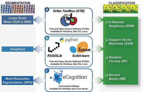
Moreover, differently from previous research works dealing with the comparison of GEOBIA approaches (De Luca et al., 2019; M. Li et al., 2016b; Qian et al., 2015; Teodoro & Araujo, 2016; Vilar et al., 2020), we implemented the segmentation step using three different algorithms. The Large Scale Mean-Shift (LSMS) (Michel et al., 2015) in OTB, the Shepherd algorithm in the Image Segmentation Module of the RSGISLib (Shepherd et al., 2019), and the Multi-Resolution Segmentation (MRS) algorithm (Baatz & Schape, 2000) in eCognition.

A workflow was carried out on two different study sites characterized by two different crops, both socioeconomically relevant for the investigated area. The first study site (Orchard-study site) is a citrus orchard of bergamot (Citrus bergamia, Risso), labeled with the protected designation of origin (PDO) label Bergamotto di Reggio Calabria – olio essenziale (“Bergamot of Reggio Calabria – essential oil”). The second study site (Crop-study site) is an onion crop field (Allium cepa L.), labeled with the protected geographical indication label “Cipolla Rossa di Tropea IGP” (“Tropea’s Red Onion PGI”).

To our best knowledge, this research is the first that compares four machine learning algorithms implemented in three different software environments and therefore using three different segmentation algorithms. The aim was to implement a rapid and reliable agricultural mapping, easily replicable in different operational scenarios with minor changes.

This paper is structured as follows. In Section 2, in the first subsection (2.1), a description of the two investigated study sites was provided. The following subsection (2.2) shows the details about data acquisition, the sensor used, and flight data processing. The used software environments were briefly described in addition to the pre-processing, segmentation, and classification steps. Section 3 provides the results of segmentation and classification processes taking into consideration the obtained accuracy. Finally, sections 4 and 5 deal with discussions and conclusions, respectively.

Materials and methods

Study sites

The Orchard-study site (Figure 2) is a citrus orchard (bergamot, Citrus bergamia) located in Palizzi (Province of Reggio Calabria, Calabria, Italy) (37°55ʹ06‖N, 15°58ʹ54‖E, 4 m a.s.l). Inside the orchard, there are long windbreak barriers made up of 20-year-old olive trees. The area where the orchard lies is 5.1 ha. The citrus orchard includes trees aged 5 to 25 years, which height ranges between 1.5 to 4 m, while canopies occupy a mean area of 6 m². The windbreak barriers include trees with a height similar to neighboring citrus trees (age 25 years).

Figure 2. Geographical location of the two study sites, Orchard-study site, and Crop-study site. On the bottom, we provided two representative photos of them

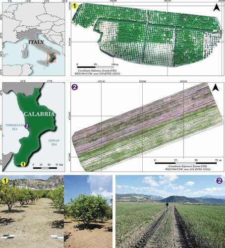
Crop-study site (Figure 2) is an onion crop located in Campora S. Giovanni, in the municipality of Amantea (Cosenza, Italy, 37°55ʹ06” N, 15°58ʹ 54” E, 4 m a.s.l.). The farm is part of a consortium that includes other producers whose total cultivated area under the onion crop is more than 500 ha. The onions produced are a relevant typical product for this area’s economic and rural development (Messina et al., 2020a, 2020b). The study area examined is a field of 1 ha. The field is crossed by four paths of 2.5 m each, used for agricultural vehicles’ passage. Inside the field, the presence of weeds whose manual removal is carried out periodically is visible. Typically, the onions transplant took place in early September, while the harvest occurred from mid to the end of January.

Sensors and data acquisition

Imagery for the two study sites was acquired using the Tetracam µ-MCA06 snap (Tetracam Inc. – Chatsworth, NJ, USA) mounted on a multirotor UAV (Multirotor G4 Surveying Robot – Service Drone GmbH). The µ-MCA06 snap is a six sensors narrow-band multispectral camera equipped with its own global navigation satellite system (GNSS). Each sensor shoots simultaneously, and all images are then synchronized via the master channel (Table 1).

Table 1. Tetracam µ-MCA06 snap (Global shutter) sensor characteristics bands specification (wavelength and bandwidth)

Geometry of lens	Sensors	Bands	Central band wavelength [nm]	Bandwidth[nm]
Focal Length (fixed lens) 9.60 mm	Master (0)	Near-Infrared 1 (NIR1)	800	10
Dimension 6.66 mm x 5.32 mm	1	Blue (B)	490	10
1.30 Megapixel CMOS	2	Green (G)	550	10
4:3 format 1280 × 1024 pixels	3	Red (R)	680	10
Pixel size 4.80 microns	4	Red-edge (RE)	720	10
Angle of View (W x H) 38.26° x 30.97°	5	Near-Infrared (NIR2)	900	20

Due to the different characteristics of the analyzed crops in the two study sites (an orchard and an annual crop), we carried out the surveys with different flight altitudes, 80 and 30 m a.g.l. for Orchard and Crop study sites, respectively. Consequently, the GSD was 4.1 cm for the Orchard-study site and 1.5 cm for the Crop-study site (Table 2). All flights were operated under constant scene illumination and cloud-free conditions.

Table 2. Flights and UAV datasets characteristics

Study site	Date	Flight height [a.g.l.]	Take-off time[UTC+1]	Speed [m s^−1]	N° of flights	Total duration[min]	Surveyed area [ha]	Photos[n°]	Sidelap and Endlap [%]	Ground sample distance (GSD) [cm]	Field of View (FOV) [m]	RMSE [m]
												X	Y	Z
Orchard	2018/09/17	80 m	11:00 am	2.50	2	49	5.13	2825	80	4.10	55.50 x 44.33	0.03	0.03	0.09
Crop	2019/11/21	30 m	12:00 am	2.50	1	19	1.01	1800	80	1.50	20.81 x 16.63	0.02	0.02	0.05

All the acquired images were first extracted and then aligned, stacked, and radiometrically calibrated using Pix4Dmapper Pro (version 4.3 – Pix4D SA, Switzerland). The radiometric calibration was provided using three targets (50 cm x 50 cm polypropylene panes in black, white, and grey, respectively) surveyed using the field spectroradiometer Apogee M100. After this process, a reflectance orthomosaic was produced for each of the six bands of Tetracam µ-MCA06 snap and then stacked into a single multiband orthomosaic (B, G, R, RE, NIR1, and NIR2). Moreover, a Digital Surface Model (DSM) was created after the photogrammetric process. The resolution of the DSM of the Orchard-study site is 4.1 cm/pixel, while that of the Crop-study site is 1.5 cm/pixel. For more details about the survey and the photogrammetric workflow, including the radiometric calibration process, please refer to Modica et al. (2020).

Software and libraries for the geographic object-based image analysis (GEOBIA)

OTB is an open-source toolkit developed by the French centre national d’études spatiales (CNES). It provides several applications for image segmentation and supervised or unsupervised classifiers (https://www.orfeo-toolbox.org/CookBook, last access 15 April 2021). In this research, we used the OTB version 7.0.0.

Remote Sensing and Geographical Information Systems software Library (RSGISLib) is an open-source library implemented by Bunting and Clewley in 2008 (Bunting et al., 2014). RSGISLib exploits Python language integrating a wide variety of image processing, segmentation, and object-based classification algorithms. RSGISLib uses several libraries, including GDAL, to read and write raster and vector formats (Clewley et al., 2014). In this research, RSGISLib library v.4.0.6 was used in the image segmentation step. Scikit-learn (Pedregosa et al., 2011) is another open-source package that exploits Python language integrating a wide variety of supervised and unsupervised machine learning algorithms. The Scikit-learn package covers four main topics related to machine learning: data transformation, supervised and unsupervised learning, and model evaluation (Hao & Ho, 2019; Pedregosa et al., 2011). We implemented the classification algorithms in Scikit-learn v.0.22.1 modules.

In addition, the commercial eCognition version 9.5.1 software (Trimble Inc, 2020) was used. This software allows a smooth implementation of many decision-making rules (made available by the software or customizable and implementable by the user) based on distinctive features derived from objects (Drǎguţ et al., 2014).

All packages were tested in a workstation with the following characteristics: CPU Intel Xeon E5-2697 v2, 64 GB RAM DDR3 1866 MHz, GPU NVIDIA K5000. The OTB and eCognition algorithms and the Scikit-learn modules ran under Windows 10 Pro operating system (OS) while RGISLib under Ubuntu 19.10 (Linux) OS. This was necessary since RGISLib was created and optimized for the Linux OS environment (Clewley et al., 2014; Shepherd et al., 2019).

Pre-processing and datasets

Several studies proved that the vegetation indices (VIs) enhanced spectral differences between vegetation/non-vegetation objects in UAV images (Gašparović et al., 2020; López-Granados et al., 2016; Solano et al., 2019; Torres-Sánchez et al., 2014; Villoslada et al., 2020). Even in our previous work (De Luca et al., 2019), the use of a VI, such as the normalized difference vegetation index (NDVI) (Eq. 1(Eq.1) $NDVI=\frac{\left(NIR-Red\right)}{\left(NIR+Red\right)}$(Eq.1) ) (Rouse et al., 1973), improved the classification results. Therefore, before starting the GEOBIA workflow, a green normalized difference vegetation index (GNDVI) (Eq. 2(Eq. 2) $GNDVI=\frac{\left(NIR-Green\right)}{\left(NIR+Green\right)}$(Eq. 2) ) (Gitelson et al., 1996) was calculated for both datasets to increase the spectral information.

(Eq.1) $NDVI=\frac{\left(NIR-Red\right)}{\left(NIR+Red\right)}$(Eq.1)

(Eq. 2) $GNDVI=\frac{\left(NIR-Green\right)}{\left(NIR+Green\right)}$(Eq. 2)

We used this index, considering its higher sensitivity to the chlorophyll concentration than NDVI (Candiago et al., 2015; Gitelson & Merzlyak, 1998) and its high correlation also with other VIs such as the normalized difference red edge index (NDRE), the soil adjusted vegetation index (SAVI), and the green-red normalized difference vegetation index (GRNDVI), as in the case of our two analyzed datasets (Supplementary material, Figure S1).

For all the six bands of the orthomosaic and both GNDVI and DSM layers, a linear band stretching (rescale) in a range of 8 bits [0, 255] was performed. This operation aimed to equalize the range of values of each input variable, reducing the influence of differences in their magnitudes and the effect of potential outliers (Angelov & Gu, 2019; Immitzer et al., 2016). Subsequently, a layer stacking process was performed by merging the original six bands with GNDVI and DSM. Finally, each of the two datasets resulted in an eight-band orthomosaic: blue (B), green (G), red (R), red edge (RE), near-infrared 1 (NIR1), near-infrared 2 (NIR2), GNDVI and DSM. All these bands were used for all segmentation and classification processes.

Image segmentation algorithms

In the GEOBIA approach, image segmentation is the first process that fragments a digital image into a set of spatially adjacent segments composed of a group of pixels presenting homogeneous features (radiometric, geometric, etc.). Each object on the segmented image should represent a real object on the earth’s surface (Blaschke et al., 2014). In this study, three different segmentation approaches, each corresponding to the three different software environments, were implemented for each of the two datasets. Table 3 shows the values concerning each algorithm’s main input parameters set for each and based on previous experiences (De Luca et al., 2019; Modica et al., 2020), a thorough exploration of the literature, and a trial-and-error approach.

Table 3. Main segmentation parameters implemented in each segmentation algorithm (Large-scale mean shift, LSMS; Shepherdalgorithm.; multi-resolution segmentation, MRS) and for both study sites

Algorithms	Parameter	Orchard-study site	Crop-study site
LSMS	Tile size (number of pixels)	500 x 500	1000 x 1000
	Spatial radius	5	5
	Range radius	4	3
	Minimum region size (in pixels)	165	15
Shepherd algorithm	Number of clusters	200	90
	Minimum number of pixels within a segment	460	18
	Spectral distance threshold (i.e., to merge neighboring segments)	100	125
	Number of subsampling	100	70
	Number of maximum iterations	3000	3000
MRS	Shape	0.10	0.10
	Compactness	0.50	0.50
	Scale	30	5

Large-scale mean-shift (LSMS)

LSMS is a segmentation workflow introduced by Fukunaga and Hostetler (1975) and subsequently developed by Michel et al. (2015). It consists of a series of dedicated and optimized algorithms that perform a tile-wise segmentation of extensive VHR imagery (www.orfeo-toolbox.org/CookBook; Michel et al., 2015). The LSMS workflow is composed of four successive steps that produce a vector file with artifact-free polygons. Each polygon corresponds to segmented objects containing the radiometric mean and variance of each band. The provided workflow can be synthesized as follow. The first step (1) performs an image smoothing using the LSMS-Smoothing application. In the second step (2), the LSMS-Segmentation algorithm segments the image grouping of all neighboring pixels based on a range distance (range radius) and a spatial distance (spatial radius). The range radius is defined as the threshold of the spectral signature Euclidean distance among features (expressed in radiometry units), while the spatial radius defines the maximum distance to build the neighborhood from averaging the analyzed pixels. Several trial-and-error tests of different range radius values were performed until the best segmentation (visually assessed) was obtained. In the third step (3), LSMS-Merging, the small objects are merged with the nearest radiometrically more similar ones. The last step (4), LSMS-Vectorization, concerns the vectorization of the merged image objects. In the final output, the mean and standard deviation of spectral features are provided for each polygon. The set parameters are shown in Table 3.

Shepherd algorithm

Image segmentation on Python was executed using the Shepherd algorithm (Shepherd et al., 2019) implemented in the RSGISLib v4.0.6. This algorithm is based on an iterative elimination method, consisting of four steps: (1) A K-means clustering algorithm (MacQueen, 1967) is used for a first seeding step that identifies the unique spectral signatures within the image, assigning pixels to the associated cluster center (Z. Wang et al., 2010); (2) a clumping process creates unique regions; (3) iterative removal of that region below the minimum mapping unit threshold and merging it to the neighboring clump spectrally closest (assessed through the Euclidean distance). Finally, (4) the obtained clumps are relabeled to be sequentially numbered (Shepherd et al., 2019). Also, in this case, the following required parameters were set with a trial-and-error approach: the number of clusters requested by the K-Means algorithm, which defines the spectral separation of the segments (Shepherd et al., 2019); the minimum segment size, which represents the minimum mapping unit threshold for the elimination; and the number of maximum iterations. The segmented image was finally vectorized using the RSGISLib Vector Utils module. Feature extraction was performed with the RSGISLib Image Calculations module to obtain the mean and the standard deviation spectral features for each segment. The set parameters are shown in Table 3.

Multi-resolution segmentation (MRS)

The MRS algorithm (Baatz & Schape, 2000) implemented in eCognition is a bottom-up region-merging strategy starting with one-pixel objects (Aguilar et al., 2016). As the first step, MRS identifies single objects of a pixel’s size and then merges them with neighbor objects following a criterion of relative homogeneity. Colour homogeneity is assessed by the standard deviation of the spectral values. The deviation from a compact (or smooth) shape allows measuring the shape homogeneity. The shape parameter deals with the geometric form’s influence on the segmentation compared to the color, and its value ranges between 0 and 0.9. In contrast, the compactness parameter takes into account the combined effect of shape and smoothness. Concerning the scale parameter, several scholars showed its importance in determining the size and dimension of objects generated by the segmentation (De Luca et al., 2019; Ma et al., 2017b, 2015; Modica et al., 2020; Witharana & Civco, 2014; Yang et al., 2019). The higher the scale parameter values, the larger the obtained image objects, while, conversely, its low values resulting in smaller image objects. The set parameters are shown in Table 3.

Image classification algorithms

For each of the two study sites, the following four classification algorithms were implemented and assessed, KNN, SVM, RF, and NB. As previously described (section 2.1), we choose these two study sites with significantly diverse cultivations (i.e., an annual crop and a tree orchard) to compare the performance and the obtained results of the three different software environments and four different supervised classification algorithms. Due to these different scenarios, the classification step was implemented based on five LC classes in the Orchard-study site (i.e., Bergamot, Olive, Grass, Bare Soil, Shadows) and three LC classes in the Crop-study site (i.e., Onion, Weeds, Bare soil).

After the segmentation process, the choice of trainers is one of the most critical steps affecting the final quality of the classification results (Ma et al., 2015). Since the segmentation step was carried out autonomously in each of the three software environments, i.e., obtaining a different number and shape of segments, we selected the training objects from a shared set of points to be as objective as possible. The existing literature on training sample size and its effect on classification accuracy offers a varying range of answers to this problem, with variable results depending on several factors, such as sensor, algorithm, analyzed landscape, etc. (Ma et al., 2015; Maxwell et al., 2018; Millard & Richardson, 2015; Noi & Kappas, 2018; Qian et al., 2015; Ramezan et al., 2021). In practice, the number of object-based training samples is usually determined based on the user experience (Qian et al., 2015). However, these studies commonly observed that different algorithms become insensitive to the increase of sample size: e.g., in Qian et al. (2015), this happened (for all the KNN, NB, SVM, and DT algorithms) when the size of the samples is more than 125 per class. Therefore, to train each of the four supervised algorithms, two samples of 800 and 500 points for Orchard and Crop study sites, respectively, were randomly sampled on the QGIS environment. The total number of random points was chosen to potentially have about 160 training samples per class for both study sites. Considering the high number of sample points, the random sample approach allows that the number of trainers per class to be almost proportional to their abundance and quantitative distribution on the scene, thus avoiding that individual classes become over-represented (Maxwell et al., 2018; Millard & Richardson, 2015; Ma et al., 2015). Additionally, to accept the resulting distribution, we fixed as a threshold that each class must be represented by at least 5% of the total number of trainers (40 for the Orchard-study site and 25 for the Crop-study site). We used this threshold based on the work of Noi and Kappas (2018) that used this percentage as a minimum training size in their tests achieving good accuracy results with SVM, RF and KNN, while the tests by Qian et al. (2015) showed that good accuracy levels can still be reached with a number of 25 trainers per class using SVM, KNN, NB and Decision Tree algorithms.

Subsequently, these points were superimposed on each of the three obtained segmentation output files to select and extract by position the polygons that include them. These selected polygons were then labeled with the corresponding LC class by an on-screen interpretation done by the same operator. The visual interpretation was supported by a good knowledge of the two study sites by the operator. All the pixels that composed a reference polygon belonged to a specific LC for all three segmentation results. Each LC class’s spectral signatures were characterized based on the respective training polygons for each of the three software environments (Supplementary material, Figure S2). Moreover, for each training polygon, we extracted the features’ objects (mean and standard deviation). The KNN is a non-parametric supervised classifier algorithm (Aguilar et al., 2016) widely used in GEOBIA applications (Crabbe et al., 2020; Georganos et al., 2018; Griffith & Hay, 2018; K. Huang et al., 2016). This algorithm assigns a class to an object based on the class to which the neighboring objects belong in an N-dimensional feature space. The value of the parameter k defines the number of neighbors to be analyzed in the feature space, the only one to be set in the KNN that determines the classifier’s performance (M. Li et al., 2016; Qian et al., 2015). Higher values of k reduce the effect of noise in classification, although they lead to less distinction between the different classes’ boundaries, consequently a higher generalization (Maxwell et al., 2018; Trimble Inc, 2020).

The SVM is a supervised non-parametric classifier algorithm based on kernel functions belonging to the statistical learning theory algorithms (Cortes & Vapnik, 1995; Vapnik, 1998), which allows performing a multiclass classification. The SVM learns the boundary between training samples belonging to different classes to train the algorithm, projecting them into a multidimensional space and finding a hyperplane, or a set of hyperplanes that maximize the separation of the training dataset between the predefined number of classes (C. Huang et al., 2002; Mountrakis et al., 2011). In this study, we implemented a linear kernel-type function with a C model-type. The C parameter deals with misclassification size allowed for non-separable training data and regulates the training data’s rigidity (Cortes & Vapnik, 1995; Vapnik, 1998).

The RF is a machine learning algorithm proposed by Breiman (2001) and improved by Cutler et al. (2007). RF is a decisional tree’s method that randomly creates a forest comprising many decision trees, each independent from the other (M. Li et al., 2016). All the trees are trained with the same features but on different training sets derived from the original one, utilizing a bootstrap aggregation, namely bagging. The algorithm generates an internal and impartial estimation of the generalization error using “out-of-bag” (OOB) samples, which include observations that are in the original data and that do not recur in the bootstrap sample (Cutler et al., 2007). The main parameters that have to be set to determine the process performance are the number of trees, the maximum tree depth, and the minimum number of samples per node (Belgiu & Drăguţ, 2016; Breiman, 2001).

The NB is a parametric supervised classifier based on Bayes’ probability theorem (Liakos et al., 2018; Qian et al., 2015; Rehman et al., 2019) and uses a training set to calculate the probability that an object belongs to a given category or not. The algorithm estimates mean vectors and covariance matrices for every class using them for prediction. This classifier assumes that the feature data distribution function is a Gaussian mixture, one component per class (Bradski & Kaehler, 2008), and does not require parameter setting (Qian et al., 2015).

To ensure an objective comparison of the obtained classifications and the software performance, we set the same parameter values for the three classifiers (KNN, SVM, and RF) that require parameter setting, in the three software environments (OTB, Scikit-learn, and eCognition) and for both the study-sites. We tested several parameter values concerning the RF and SVM parameters based on those recommended in another previous work carried out by the same research group (De Luca et al., 2019). Moreover, in selecting the more effective values of the algorithms’ parameters, we also have taken into account several research studies that dealt with this issue (M. Li et al., 2016; Noi & Kappas, 2018; Qian et al., 2015; Rodriguez-galiano et al., 2012; H. Sun et al., 2018). In Table 4, the parameter values set for each of the three classification algorithms were reported.

Table 4. Main parameter values set in all the three software environments for each of the three implemented classification algorithms that require parameter setting, K-Nearest Neighbour (KNN), Support Vector Machines (SVM) and Random Forest (RF)

Algorithm	Parameter	Values
KNN	K (number of neighbors)	5
SVM	C (size of misclassification allowed for non-separable training data)	1
RF	Number of trees	300
	Maximum tree depth	10
	Minimum number of samples per node	1
	Number of features randomly selected for each node	The square root of the total number of features

Accuracy assessment

Segmentation accuracy assessment

In order to statistically analyze the obtained segmentations, we calculated several descriptive statistics: number, area, perimeter, etc., of the segments. Additionally, we calculated the Mean Shape Index (MSI) (eq. 3)(eq. 3) $MSI=\frac{{{{\sum }^{\hspace{0.17em}}}^{\hspace{0.17em}}}_{j=1}^N\left(\frac{p_{ij}}{\sqrt{\pi a_{ij}}}\right)}{N}$(eq. 3) by the ratio between the sum of the object perimeter (m) and the square root of the object area (m²), divided by the total number of objects, as follows:

(eq. 3) $MSI=\frac{{{{\sum }^{\hspace{0.17em}}}^{\hspace{0.17em}}}_{j=1}^N\left(\frac{p_{ij}}{\sqrt{\pi a_{ij}}}\right)}{N}$(eq. 3)

Where N is the total number of objects, p_ij is the perimeter, and a_ij the jth object area, while π is inserted as a constant value to adjust to a circular form. MSI assumes values of 1 for circular objects and increases without limits with the increasing complexity and irregularity of the analyzed objects.

Several object-based validation methods have been developed to evaluate the segmentation results (Clinton et al., 2010; Costa et al., 2018; Möller et al., 2013; Su & Zhang, 2017; Su Ye et al., 2018; Zhang et al., 2015). These are based on different objective metrics, criteria, and indices, describing and quantitatively evaluating various aspects of the obtained results. They are mainly divided into supervised and unsupervised approaches, in which they differ because the former requires a set of reference data on which to base the comparative calculations (Belgiu & Drǎguţ, 2014; Costa et al., 2018; Su & Zhang, 2017; Ye et al., 2018). Many studies evaluate the quality of segments by considering a criterion based on either geometric or non-geometric characteristics (Costa et al., 2018). Among the latter, the spectral separability through the Bhattacharyya Distance (BD) (Bhattacharyya, 1943) is one of the most used (Costa et al., 2018; D. Li et al., 2015; Radoux & Defourny, 2008; L. Wang et al., 2004; Xun & Wang, 2015). It is assumed that a good segmentation corresponds to a relatively high spectral separability between two different classes and a minimum within the polygons of the same LC class, as a function of the LC classes they represent (Costa et al., 2018).

Our study used both geometric and non-geometric metrics to have a complete characterization of the errors obtained.

In the geometric approach, each dataset’s segmentation results were evaluated by determining the geometrical similarity level with the correspondent reference object manually digitalized, using supervised geometric metrics. The comparison was carried out by overlapping and associating each reference polygon (divided by LC classes) with the respective segmented polygons using the matching criteria proposed in Clinton et al. (2010), assuming:

• X = {x_i: i = 1 … n} the set of n reference objects;

• Y = {y_j: j = 1 … m} the set of m objects deriving from the segmentation process;

• area (x_i ∩ y_j) the area of geo-intersection of reference object x_i and segmented object y_i;

• Ŷ_i a subset of Y, representing all y_j that intersect a reference object x_i such that Ŷ_i = {y_j: area(x_i ∩ y_j) ≠ 0};

• $Yi$ a subset of Ŷ_i such that:

• - Ya_i = {y_j: centroid(x_i) in y_j}

• - Yb_i = {y_j: centroid(y_j) in x_i}

• - Yc_i = {y_j: area(x_i ∩ y_j)/area(y_i) > 0.5}

• - Yd_i = {y_j: area(x_i ∩ y_j)/area(x_i) > 0.5}

so, $Y_i^{\prime }=Y{a}_{i}UY{b}_{i}UY{c}_{i}UY{d}_i$.

The validation metrics were calculated on the $Y_i^{\prime }$ set ($y_j\in Yi$).

The association criteria and subsequent geometric and non-geometric metrics were applied to the three representative square sample areas (20 m x 20 m in the Orchard-study site; 2 m x 2 m in the Crop-study site) randomly distributed over each field (Figures 3 and 4). These sample areas were sized, taking into account the different GSD (1.5 cm in the Orchard-study site and 4.1 cm in the Crop-study site) and the dimensional difference of the class objects of the two study sites. The geometric metrics used to validate the segmentation were the OverSegmentation (OSeg; eq. 4)(eq. 4) $OSe{g}_{ij}=1-\frac{area\left(x_i{\cap }^{y_j}\right)}{area\left(x_i\right)},y_j\in Yi\hspace{0.17em}$(eq. 4) and the UnderSegmentation (USeg; eq. 5)(eq. 5) $USe{g}_{ij}=1-\frac{area\left(x_i{\cap }^{y_j}\right)}{area\left(y_j\right)},y_j\in Y\hspace{0.17em}i$(eq. 5) . Moreover, these two metrics are combined using a third index, the D index (eq. 6(eq. 6) $D_{ij}=\sqrt{\frac{USe{g}^2+OSe{g}^2}{2}}$(eq. 6) ), based on their root-mean-square (Clinton et al., 2010):

(eq. 4) $OSe{g}_{ij}=1-\frac{area\left(x_i{\cap }^{y_j}\right)}{area\left(x_i\right)},y_j\in Yi\hspace{0.17em}$(eq. 4)

(eq. 5) $USe{g}_{ij}=1-\frac{area\left(x_i{\cap }^{y_j}\right)}{area\left(y_j\right)},y_j\in Y\hspace{0.17em}i$(eq. 5)

(eq. 6) $D_{ij}=\sqrt{\frac{USe{g}^2+OSe{g}^2}{2}}$(eq. 6)

Figure 3. The figure shows a comparison of the three obtained segmentations in the Orchard-study site showed in three representative sample areas. According to the three sample areas (a, b, and c), the figure is organized in three rows and in four columns. In the first column, the RGB images are provided while, in the second column, the Large-Scale Mean-Shift (LSMS) segmentation (in blue), in the third column the Shepherd algorithm segmentation (in red), and in the fourth column, the Multi-Resolution Segmentation (MRS) (in purple)

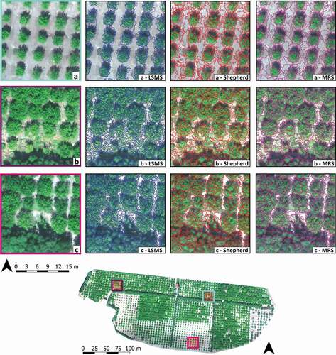
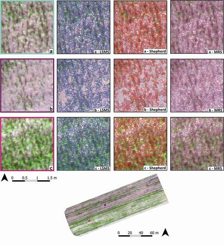
Figure 4. The figure shows a comparison of the three obtained segmentations in the Crop-study site showed in three representative sample areas. According to the three sample areas (a, b, and c), the figure is organized in three rows and in four columns. In the first column, the RGB images are provided while, in the second column, the Large-Scale Mean-Shift (LSMS) segmentation (in blue), in the third column the Shepherd algorithm segmentation (in red), and in the fourth column, the Multi-Resolution Segmentation (MRS) (in purple)

Each object $y_j\in Y\hspace{0.17em}i$ receives an individual metric value, referred to as local assessment. The assessment has been translated in global terms by averaging the values resulting from every single calculation of $Yi$ to obtain a single value that expresses the complete segmentation’s validation (Clinton et al., 2010; Costa et al., 2018). The three metrics’ values range from 0 to 1, where 0 defines the optimal overlapping (perfect segmentation) and 1 the worst. The D index can be considered a combined descriptor of the entire classification quality (Clinton et al., 2010). In an ideal case in which the segmented polygon y_j is identical to the reference one x_i, all the metrics achieve the lowest value of 0.

This study adopted the BD index (eq. 6)(eq. 6) $D_{ij}=\sqrt{\frac{USe{g}^2+OSe{g}^2}{2}}$(eq. 6) method as a non-geometric approach to validate the segmentation. It is computed as below (D. Li et al., 2015; Xun & Wang, 2015) (eq. 7(eq. 7) $BD\left(x,y\right)=2\left[1-e^{-a\left(x,y\right)}\right]$(eq. 7) –9(eq. 9) $A\left(x,y\right)=\frac{1}{2}\left[S\left(x\right)+S\left(y\right)\right]$(eq. 9) ):

(eq. 7) $BD\left(x,y\right)=2\left[1-e^{-a\left(x,y\right)}\right]$(eq. 7)

(eq. 8) $a\left(x,\hspace{0.17em}y\right)=\hspace{0.17em}\frac{1}{8}\hspace{0.17em}T\left[M\left(x\right)-M\left(y\right)\right]\hspace{0.17em}I\left[A\left(x,\hspace{0.17em}y\right)\right]\hspace{0.17em}\left[M\left(x\right)-M\left(y\right)\right]+\frac{1}{2}\hspace{0.17em}ln\left\{\frac{det\left[A\left(x,y\right)\right]}{\sqrt{det\left[S\left(x\right)\left]det\right[S\left(y\right)\right]}}\right\}$(eq. 8)

(eq. 9) $A\left(x,y\right)=\frac{1}{2}\left[S\left(x\right)+S\left(y\right)\right]$(eq. 9)

where x, y can represent the two different LC classes (i.e., interclass analysis) or two different objects of the same class (i.e., intraclass analysis). M(x) and M(y) are the matrices composed of mean reflectance values of all polygons analyzed for each spectral band. S(x) and S(y) are the covariance matrices of M(x) and M(y), respectively. T[], I[] and det[] refer to transpose, inverse, and determinant of a matrix, respectively. BD values range between 0 and 2, with higher values representing higher (i.e., better) separability.

The mean BD value was calculated for each segmentation resulting from the different algorithms through the average of the BDs calculated between the defined LC classes (interclass analysis). Then, the BD was calculated iteratively among the various polygons of the same class. The obtained values were averaged to have BD’s mean value for each class (intraclass analysis).

Classification accuracy assessment

For all the tested GEOBIA classifications, a sample of 500 random points was created for each of the two datasets scenes to carry out a proper classification accuracy validation. We implemented the simple random sample selection of these points considering that we compared different classification algorithms, whose classifications could lead to different class compositions. Other sample schemes, such as stratified random or equalized stratified random sampling, would require higher user influence and a priori knowledge of area and position occupied by each class, decreasing the objectivity of the comparison and increasing processing times. In an operational workflow of PA, stratified random schemes would not be suitable in terms of cost and benefits. Furthermore, given the very high number of sample points (500) randomly distributed over the whole scene, they represent a good sample, also in terms of class composition.

Every point was labeled according to the defined LC classes by visual interpretation (reference truth). Subsequently, for each of the four classifiers and in each of the three different segmented vector layers, all polygons containing the sampling points were selected. For each of them, the reference truths were compared with the classified LC class. The producer’s accuracy (the ratio between the correctly classified objects in a given class and the number of validation objects for that class), the user’s accuracy (the ratio between the correctly classified objects in a given class and all the classified objects in that class), and the overall accuracy (OA) (i.e., the total percentage of correct classification) were calculated (Congalton & Green, 2019). Finally, from these measures, we calculated the F-score (Goutte & Gaussier, 2005; Ok et al., 2013; Shufelt, 1999; Sokolova et al., 2006) for every single class (F_i) (eq.10)(eq. 10) $F_i=2\frac{produce{r}^{\prime }{s}_{i}use{r}^{\prime }{s}_i}{produce{r}^{\prime }{s}_i+use{r}^{\prime }{s}_i}$(eq. 10) and the multi-class F-score (F_M) (eq. 11(eq. 11) $F_M=2\frac{produce{r}^{\prime }{s}_{M}use{r}^{\prime }{s}_M}{produce{r}^{\prime }{s}_M+use{r}^{\prime }{s}_M}$(eq. 11) ) (Sokolova & Lapalme, 2009) that represents the mean of all LC classes.

The F-score represents the harmonic mean of its components, recall (r), and precision (p). Considering that r and p have the same meaning of producer’s and user’s accuracy, respectively, they were replaced in equations 10(eq. 10) $F_i=2\frac{produce{r}^{\prime }{s}_{i}use{r}^{\prime }{s}_i}{produce{r}^{\prime }{s}_i+use{r}^{\prime }{s}_i}$(eq. 10) and 11(eq. 11) $F_M=2\frac{produce{r}^{\prime }{s}_{M}use{r}^{\prime }{s}_M}{produce{r}^{\prime }{s}_M+use{r}^{\prime }{s}_M}$(eq. 11) . The F_i and the F_M share the same formula (eq. 10(eq. 10) $F_i=2\frac{produce{r}^{\prime }{s}_{i}use{r}^{\prime }{s}_i}{produce{r}^{\prime }{s}_i+use{r}^{\prime }{s}_i}$(eq. 10) and 11(eq. 11) $F_M=2\frac{produce{r}^{\prime }{s}_{M}use{r}^{\prime }{s}_M}{produce{r}^{\prime }{s}_M+use{r}^{\prime }{s}_M}$(eq. 11) ).

(eq. 10) $F_i=2\frac{produce{r}^{\prime }{s}_{i}use{r}^{\prime }{s}_i}{produce{r}^{\prime }{s}_i+use{r}^{\prime }{s}_i}$(eq. 10)

(eq. 11) $F_M=2\frac{produce{r}^{\prime }{s}_{M}use{r}^{\prime }{s}_M}{produce{r}^{\prime }{s}_M+use{r}^{\prime }{s}_M}$(eq. 11)

Where i is a single LC class and n the total number of LC classes while the producer’s_M accuracy is as follows (eq. 12)(eq. 12) $produce{r}^{\prime }{s}_M=\frac{{\sum }_{i=1}^{n}producer{ }^{\mathrm{\prime }}{s}_i}{n}$(eq. 12) :

(eq. 12) $produce{r}^{\prime }{s}_M=\frac{{\sum }_{i=1}^{n}producer{ }^{\mathrm{\prime }}{s}_i}{n}$(eq. 12)

And user’s_M accuracy is (eq. 13)(eq. 13) $use{r}^{\prime }{s}_M=\frac{{\sum }_{i=1}^{n}use{r}^{\prime }{s}_i}{n}$(eq. 13) :

(eq. 13) $use{r}^{\prime }{s}_M=\frac{{\sum }_{i=1}^{n}use{r}^{\prime }{s}_i}{n}$(eq. 13)

Statistical comparison between classification results: McNemar’s test

An additional objective comparison was carried out in order to evaluate the relative significance of differences observed between classifications, the McNemar’s test (Dietterich, 1998; McNemar, 1947; Foody, 2004). It is a non-parametric test based on a contingency table of 2 × 2 dimension constructed using the binary distinction between correct and incorrect class allocations, widely used to determine if statistically significant differences are present between pairs of classifications (Y. Gao et al., 2011); Millard & Richardson, 2015; Quan et al., 2020; Belgiu & Csillik, 2018; Kavzoglu, 2017; Dietterich, 1998; Sokolova et al., 2006). This test is suitable to assess the difference of multiple classification accuracy performances when the same set of validation and training samples are used (Foody, 2004; Y. Gao et al., 2011). Supposing the comparison of two classification outputs (a and b), the McNemar’s test can be expressed as (eq. 14)(eq. 14) $z^2=\frac{{(|f_{ab}-f_{ba}|-1)}^2}{f_{ab}+f_{ba}}$(eq. 14) :

(eq. 14) $z^2=\frac{{(|f_{ab}-f_{ba}|-1)}^2}{f_{ab}+f_{ba}}$(eq. 14)

Where f_ab is the number of validation samples incorrectly classified by classification a but correctly classified by the classification b, and f_ba the number of validation samples incorrectly classified by classification b but correctly classified by classification a. McNemar’s test uses a Chi-squared distribution with one degree of freedom (Dietterich, 1998; Foody, 2004), and the associated p-value is calculated. A p-value smaller than 0.05 indicates that the differences between the two observations a and b are statistically significant, while a p-value higher than 0.05 indicates that the differences between the two observations are statistically not significant.

The contingency table was constructed using the validation polygons already employed for accuracy assessment. Considering the comparison of each pair combination of classifications, the four values that constitute the 2 × 2 contingency table are: i) the number of polygons correctly classified by both classifications (Yes/Yes); ii) the number of polygons incorrectly classified by both classifications (No/No); iii) the number of polygons correctly classified by the first classification but incorrectly classified by the second classification (Yes/No); iv) the number of polygons incorrectly classified by the first classification but correctly classified by the second classification (No/Yes). The McNemar’s test was computed using the contingency_tables.mcnemar function of the Python module statsmodule.

Results

Analysis and comparison of the obtained segmentations

To quantitatively assess the segmentation performance, several geometric (OSeg, USeg and D index) and non-geometric (BD) metrics were computed for each algorithm and dataset how explained in Section 2.7.1. Before that, each process was timed, a series of descriptive metrics were calculated and compared, and a prior visual assessment was carried out. To show the different segmentations obtained using LSMS, Shepherd and MRS algorithms, in Figures 3 and 4, we reported the three representative subsets in which the segmentation accuracy was assessed. In each of them, the segmentation layer was superimposed on the RGB image using a different color for each algorithm, blue (LSMS), red (Shepherd algorithm), and purple (MRS).

For each of the three implemented segmentation algorithms and the two study sites, Table 5 reports the processing time, the number of segments, and the following main characteristics of obtained segments: a) area, b) perimeter, c) perimeter/area ratio, and d) mean shape index (MSI). For each characteristic, the mean (μ), the standard error (SE), and the standard deviation (σ) were provided. The processing time was calculated considering the time needed to calculate the spectral features and excluding the time required for the project preparation and parameters setting. As explained in section 2.3, the tests were performed using the same workstation.

Table 5. The table shows the most descriptive metrics of the obtained segmentations and the requested processing time for each segmentation algorithm (Large-scale mean-shift, LSMS; Shepherdalgorithm.; multi-resolution segmentation, MRS) in both study sites

Study site	Algorithm	Processing time [min.]	n° of segments	Area [m^2]		Perimeter [m]		Mean Shape Index (MSI)
				μ ± SE	σ	μ ± SE	σ	μ ± SE	σ
Orchard	LSMS	28	63,298	0.808 ± 0.036	9.013	7.894 ± 0.059	14.804	2.596 ±0.002	0.695
	Shepherd	74	25,396	2.015 ± 0.007	1.104	15.880 ± 0.045	7.123	3.170 ± 0.006	0.884
	MRS	2	35,342	1.447 ± 0.005	0.972	10.843 ± 0.026	4.830	2.639 ± 0.004	0.806
Crop	LSMS	37	1,580,899	0.0064 ± 0.00001	0.0077	0.499 ± 0.0002	0.223	1.807 ± 0.0003	0.384
	Shepherd	916	1,077,647	0.0093 ± 0.0001	0.0578	0.598 ± 0.0014	1.342	1.913 ± 0.0006	0.534
	MRS	4	1,725,819	0.0058 ± 0.00001	0.0035	0.450 ± 0.0001	0.181	1.709 ± 0.0003	0.363

μ (mean), SE (standard error), σ (standard deviation).

Referring to both study sites, the processing time lasted, respectively, 28 and 37 minutes using LSMS, 74 and 916 in Shepherd algorithm, 2 and 4 minutes using MRS. In the Orchard-study site, the segmentation processes provided a number of segments ranging from 25,396 (Shepherd algorithm) to 63,298 (LSMS). The MRS algorithm produced 35,342 segments. In the Crop-study site, the number of segments ranging from 1,077,647 of the Shepherd algorithm to 1,725,820 of the MRS algorithm, while the LSMS produced 1,580,899 segments. In this study site, both MRS and LSMS segmentation algorithms produced a similar and large number of segments compared to those obtained using the Shepherd algorithm. These aspects can be noticed looking at the values of the mean perimeter length of the segments and, in the same case, the shape of the single segments seems to be very similar, according to the close values of MSI. The total number of segments and their mean area (in m²) with standard deviation, reported in Table 5, gives a useful general measure of the relationship between size and number of image objects, which has a direct impact on the subsequent classification steps (Ma et al., 2015; Torres-Sánchez et al., 2015a). The mean segment size, as more detailed in Table 5, varies between 0.81 ± 0.04 m² (σ = 9.01) (LSMS) and 2.02 ± 0.01 m² (σ = 1.10) (Shepherd algorithm), and between 0.006 ± 0.00 m² (σ =0.008) (LSMS) and 0.009 ± 0.00 m² (σ = 0.06) (Shepherd algorithm), for Orchard and Crop study sites, respectively. The mean perimeter length follows the trend of the mean segment size, varying from 7.89 ± 0.06 m (σ = 14.80) (LSMS) and 15.88 ± 0.05 m (σ = 7.12) (Shepherd algorithm) for Orchard-study site, and between 0.45 ± 0.00 m (σ = 0.18) m (MRS) and 0.60 ± 0.00 m (σ = 1.34) (Shepherd algorithm), for Crop-study site. MSI result is very similar for segmentations obtained using LSMS and MRS in the Orchard-study site (2.60 and 2.64, respectively). Similarly, it is higher for the Shepherd algorithm (3.17), therefore denoting segments more complex and more irregular than the other two algorithms. In the Crop-study site, the obtained segments are more compact and homogeneous. This is true especially for MRS and LSMS algorithms (MSI of 1.71 and 1.81, respectively), while the Shepherd algorithm led to objects with more irregular geometries (MSI = 1.913).

Table 6 shows the supervised segmentation metrics (i.e., geometric and non-geometric) calculated for each study site and algorithm. These included two geometric metrics, that is, OSeg, USeg, representing over- and under-segmentation errors calculated separately and combined later to provide a third complementary metric, the D index. The non-geometric BD expresses the spectral separability between polygons and is defined at inter- and intra-class levels.

Table 6. Segmentation accuracy obtained applying the three geometric segmentation indices (OSeg, OverSegmentation; USeg, UnderSegmentation; D index) and the non-geometric segmentation index (BD, Bhattacharyya index) at inter- and intra-class level. Data are referred to the three sample areas in each study site and for each of the three segmentation algorithms (Large-scale mean-shift, LSMS; Shepherd algorithm.; multi-resolution segmentation, MRS)

		Geometric segmentation metrics			Non-geometric segmentation metrics
Study site	Algorithms	OSeg	USeg	D index	BD (inter-class)	BD (intra-class)
Orchard	LSMS	0.724	0.201	0.587	1.675	0.605
	Shepherd	0.652	0.222	0.581	1.767	0.586
	MRS	0.674	0.207	0.571	1.660	0.658
Crop	LSMS	0.643	0.175	0.531	1.639	0.607
	Shepherd	0.625	0.205	0.541	1.634	0.803
	MRS	0.668	0.142	0.526	1.640	0.584

The segmentation evaluation metrics indicated a large discrepancy between over- and under-segmentation errors but with very similar behavior for all three algorithms in both study sites. It is evident how OSeg remains high in both study sites, never going below 0.625 (Shepherd algorithm., in Crop-study site), with a maximum value reached by LSMS in Orchard-study site (0.724). The USeg values are low for all the three algorithms and both study sites, ranging from 0.142 (MRS in Crop-study site) to 0.222 (Shepherd algorithm in Orchard-study site). For both study sites, the highest values of the USeg index concerned the Shepherd algorithm (0.222 and 0.205, respectively). The D index’s highest value was reached in the Orchard-study site by LSMS (0.724); the same study site’s lower value was obtained with the MRS algorithm (0.571). In the Crop-study site, the D index reached the lowest value (0.526) using the MRS algorithm.

The BD, which expresses the mean spectral separability, as detailed in section 2.7, was calculated both between the different LC classes (BD inter-class) and between the same LC class’s polygons (BD intra-class). The results show how the segmented polygons have a high average separability between different classes, finding very similar values between the various algorithms and study sites (values ranging from 1.634 to 1.767). Within the same LC class, the spectral separability remains low with a minimum value of 0.584 for MRS and the highest value of 0.803 for the Shepherd algorithm, both in the Crop-study site.

Classification accuracy overview

A synoptic accuracy overview of the obtained results for all the four implemented classifiers was provided in Figures 5 and 6, expressed as overall, producer’s and user’s accuracy values, and Fi (single-class) F_M (multi-class) values.

Figure 5. Orchard-study site. User’s, Producer’s and Overall accuracies, and F-score_i (single-class) and F-score_M (multi-class) values obtained for each algorithm (K-Nearest Neighbour, KNN; Support Vector Machines, SVM; Random Forests, RF; Normal Bayes, NB) in every software environment (Orfeo ToolBox, OTB; Scikit-learn; eCognition)

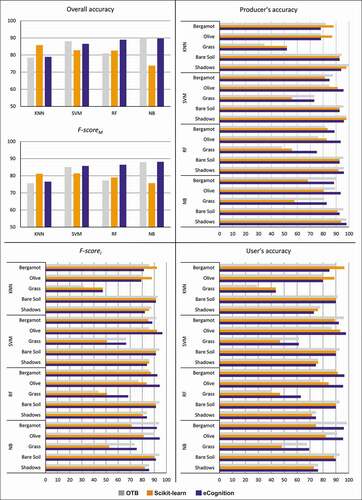
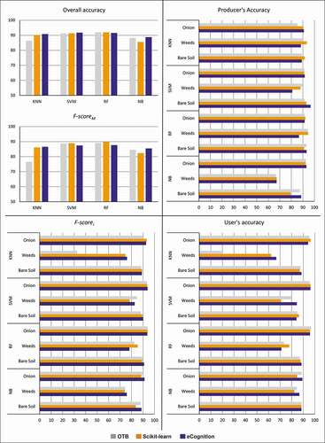
Figure 6. Crop-study site, user’s, producer’s and overall accuracies, and F-score_i (single-class) and F-score_M (multi-class) values obtained for each algorithm (K-Nearest Neighbour, KNN; Support Vector Machines, SVM; Random Forests, RF; Normal Bayes, NB) in every software environment (Orfeo ToolBox, OTB; Scikit-learn; eCognition)

Moreover, 4 columns x 3 rows of visual comparison matrices were implemented to comprehensively picture the obtained image classification results in the two study sites (Figures 7 and 8). In these matrices, images are organized according to the four classification algorithms in matrix columns (KNN, SVM, RF and NB) and the three software environments (OTB, Scikit-learn and eCognition) in matrix rows. To this end, we choose two sample areas of the whole scenes for each of the two study sites to show and visually compare the obtained classifications (Figures 7 and 8).

Figure 7. Orchard-study site. The figure reports two visual comparison matrices showing the obtained classification results in two significant portions of the whole scene (a and b). Their visualization in visible (RGB), and their localization on the study site are provided on the top side. In each of the two visual matrices (a and b), the images are organized according to the four classification algorithms, K-Nearest Neighbour (KNN), Support Vector Machines (SVM), Random Forests (RF), and Normal Bayes (NB) (matrix columns), and the three software environments, Orfeo ToolBox (OTB), Scikit-learn and eCognition (matrix rows)

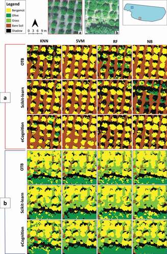
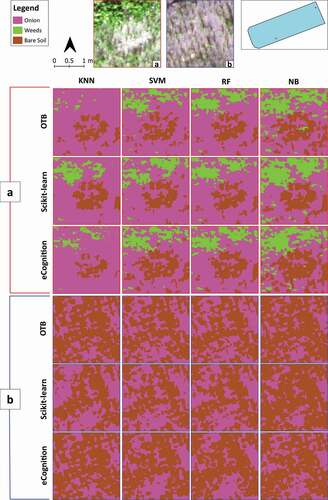
Figure 8. Crop-study site. The figure reports two visual comparison matrices showing the obtained classification results in two significant portions of the whole scene (a and b). Their visualization in visible (RGB), and their localization on the study site are provided on the top side. In each of the two visual matrices (a and b), the images are organized according to the four classification algorithms, K-Nearest Neighbour (KNN), Support Vector Machines (SVM), Random Forests (RF), Normal Bayes (NB) (matrix columns), and the three software environments, Orfeo ToolBox (OTB), Scikit-learn and eCognition (matrix rows)

OA and FM’s highest values were obtained in the Orchard-study site using the NB algorithm, 89.68% and 89.76% (OA) on OTB, and 87.88% and 88.15% (F_M), on eCognition. The same algorithm performed the lowest values on Scikit-learn (73.80% and 75.73%, for OA and F_M, respectively). The SVM and RF algorithms follow at performance level with slightly lower OA values on eCognition (86.57% and 88.96%, respectively) and gradually lower on OTB (88.0% and 81.0%) and Scikit-learn (82.80% and 82.60%, respectively). In Scikit-learn, the highest OA was reached by the KNN algorithm, while the F_M^’ highest value with SVM.

OA of RF and SVM was above 90% in all three software suites in the Crop-study site. For the other two algorithms, KNN and NB, the lowest OA performance was achieved on OTB and Scikit-learn, respectively. Observing the single class accuracies, in the Bergamot class, the highest F_i value was found using the NB algorithm on OTB (93.95%) while the respective user’s accuracy was 98.46%, and the producer’s accuracy corresponded to 89.82%. As for the Olive class, the highest values of accuracies were reached by SVM performed on eCognition (97.78%, 95.65%, and 96.70% for user’s, producer’s, and F_i accuracies, respectively). We found the lowest user’s accuracy values in the Grass class, ranging from 29.03% (KNN on OTB) to a maximum value reached in eCognition by the NB classifier (69.35%). The F_i follows the trend with the lowest value equal to 31.58% (KNN on OTB). Focusing on the Shadows LC class, the producer’s accuracy never falling below 91.84%, reaching 100% using the KNN algorithm implemented on OTB. The users’ accuracy has lower values but showed the same trend, as well as F_i, whose highest value is 87.50% (KNN on OTB).

In the Crop-study site, as for the Onion class user’s accuracy values, there are not many differences in the obtained results of the implemented algorithms in the different software environments, maintaining averaged values around 95.0%. Only with the NB algorithm, slightly lower values were obtained. All the algorithms performed values of the producer’s accuracy higher than 90.0%, except for KNN implemented on OTB (85.27%). The F_i has values not lower than 90.0% except for NB on Scikit-learn (88.45%). As far as the Weeds class is concerned, the highest values of the user’s accuracy were obtained using NB (86.67%) and SVM (84.44%), both performed in eCognition. We obtained the lowest value implementing KNN in OTB, which provided a value of 20.0%.

The difference in accuracy between every pair of classifications was statistically analyzed using McNemar’s test. In total, 66 combinations of classification were statistically compared for each study site. In Tables 7 and 8 are reported the resulted p-values for each classification pair, indicating when the difference was statistically non-significant (p-value > 0.05) or significant (p-value < 0.05). For the Orchard-study site, the accuracy results of NB, performed in Scikit-learn, are significantly different from those of all other classifications. Similar results are showed for KNN of OTB and eCognition. On the other hand, NB, used through the other two software, showed similitude with SVM. Regardless of the software used, the two classifiers RF and SVM, show multiple boxes with p-value > 0.05 compared to each other. The KNN of Scikit-learn did not express significant differences when compared to most other classifications. For the Crop-study site, the NB still maintains statistically significant differences with most of the other classifications. However, there are more statistical similarities between the different classification results. The RF and SVM achieved no significant differences in all software, with SVM of eCognition showing no difference (p-value = 1) than RF of all three software.

Table 7. McNemar’s Test p-values obtained comparing the classification accuracy results of each couple of classifications (combination of software + classifier) in the Orchard-study site. The values indicate when the difference between two classifications accuracy results are statistically significant (p-value < 0.05) or not-significant (p-value > 0.05)

KNN

OTB

Scikit-learn

< 0.05

eCognition

0.419

< 0.05

SVM

OTB

< 0.05

0.235

< 0.05

Scikit-learn

< 0.05

0.826

< 0.05

0.107

eCognition

< 0.05

0.501

< 0.05

0.586

0.278

RF

OTB

< 0.05

0.149

0.073

< 0.05

0.219

< 0.05

Scikit-learn

< 0.05

0.337

< 0.05

< 0.05

0.494

0.089

0.555

eCognition

< 0.05

0.108

< 0.05

0.752

< 0.05

0.295

< 0.05

< 0.05

NB

OTB

< 0.05

0.390

< 0.05

0.822

0.265

0.850

< 0.05

0.080

0.562

Scikit-learn

< 0.05

< 0.05

< 0.05

< 0.05

< 0.05

< 0.05

< 0.05

< 0.05

< 0.05

< 0.05

eCognition

< 0.05

0.533

< 0.05

0.614

0.351

1.000

< 0.05

0.117

0.275

0.842

< 0.05

OTB

Scikit-learn

eCognition

OTB

Scikit-learn

eCognition

OTB

Scikit-learn

eCognition

OTB

Scikit-learn

eCognition

KNN

SVM

RF

NB

Table 8. McNemar’s Test p-values obtained comparing the classification accuracy results of each couple of classifications (combination of software + classifier) in the Crop-study site. The values indicate when the difference between two classifications accuracy results are statistically significant (p-value < 0.05) or not-significant (p-value > 0.05)

KNN

OTB

Scikit-learn

< 0.05

eCognition

< 0.05

0.749

SVM

OTB

< 0.05

0.878

0.551

Scikit-learn

< 0.05

0.064

< 0.05

0.251

eCognition

< 0.05

0.533

0.243

0.711

0.442

RF

OTB

< 0.05

0.377

0.122

0.541

0.541

1.000

Scikit-learn

< 0.05

0.327

0.122

0.557

0.503

1.000

1.000

eCognition

< 0.05

0.636

0.189

0.868

0.405

1.000

0.839

0.845

NB

OTB

0.349

0.136

0.220

< 0.05

< 0.05

< 0.05

< 0.05

< 0.05

< 0.05

Scikit-learn

0.731

< 0.05

< 0.05

< 0.05

< 0.05

< 0.05

< 0.05

< 0.05

< 0.05

0.160

eCognition

0.188

0.253

0.371

0.119

< 0.05

< 0.05

< 0.05

< 0.05

< 0.05

0.788

0.064

OTB

Scikit-learn

eCognition

OTB

Scikit-learn

eCognition

OTB

Scikit-learn

eCognition

OTB

Scikit-learn

eCognition

KNN

SVM

RF

NB

Discussion

Performance of the different segmentation algorithms

In line with the results of Clewley et al. (2014), the MRS algorithm was the fastest for both study sites, with a processing time ranging from 2 minutes (Orchard-study site) to 4 minutes (Crop-study site). However, the open-source OTB, which allows setting the available RAM for a running process during each of the four segmentation steps, performed good processing times (28 and 37 minutes for Orchard and Crop study sites, respectively). LSMS and Shepherd algorithms perform a tile-based segmentation, and both OTB and RSGISLib are designed to optimize RAM and CPU usage. However, although RSGISLib completed the segmentation process in few minutes for both study sites (about 7 minutes for both cases), the extraction of the spectral features of each segment (mean and standard deviation) required almost all the process-time on the Crop-study site (lasted more than 15 hours). Indeed, the considerable number of segments led to a critical slowdown of the system in RSGISLib. Moreover, Python language does not use all multi-processors by default (mono-thread). This leads to a slowdown of the high-magnitude computational processes. Several approaches can be implemented to solve this problem to make the program using the entire CPU and/or GPU computing capabilities (e.g., multiprocess, multithread, CUDA) (Gorelick & Ozsvald, 2020). However, their use requires experienced programming operators and, for now, is beyond our research aims.

The segmentation results differ in the number and size of the obtained segments, but this was expected since all three software exploited different algorithms. In the Orchard-study site, the LSMS provided the highest number of segments (mean area of 0.81 m²), about double that of the other two algorithms. Consequently, compared to the Shepherd algorithm and MRS algorithms, the segment size differences were particularly evident. This is corroborated by the higher standard deviations of mean segment size and perimeter (±9.01 and ±14.80, respectively). This is also reflected in the over-segmentation errors, which for LSMS are higher than the other two (Table 6). However, observing Figure 3, it would seem that LSMS has been able to segment better in some cases and thus represent the various and heterogeneous shapes of the objects. For example, a single shadow or a bare soil object among the vegetation corresponds to a single segment, closely corresponding to its actual shape (Figure 2a-LSMS). Where the ground surface was continuous, larger segments were generated (with two segments covering more than 500 and 2000 m², respectively).

Meanwhile, a tree canopy and other vegetation covers have been split into many more segments than the other two algorithms. This can be explained by the different behavior of the scene’s features, as De Castro et al. (2018) have shown. Indeed, the soil and the shadows had more similar spectral characteristics than the vegetation, spectrally and structurally heterogeneous. The irregular structure of the vegetational cover affected these surfaces’ spectral variability. This condition is particularly evident in VHR images, where it is expected that many segments are composed of heterogeneous regions (Hossain & Chen, 2019; Torres-Sánchez et al., 2015a).

On the other hand, the bare soil’s homogeneous reflectance behavior could be due to its smoothed surface (low roughness). The same behavior, with less evidence, can also be noticed in the Shepherd algorithm segmentation.

The variation in segment size was not particularly evident in the Crop-study site, confirmed by a standard deviation that never exceeds 0.06 m² (Table 5). Indeed, the MSI index reaches lower values than the Orchard-study site, which means less irregularly-shaped segments. This was due to vegetation’s size and structure (herbaceous), which were more homogeneous than the Orchard-study site (trees and grasses). Moreover, in the Orchard-study site, the bergamot trees have different ages (from 5 to 25 years old) along the field, leading to a greater diversification of the crowns’ size. Table 5 shows that the number of segments is compared to the mean object size, which can be considered a representation of the segmentation scale (Torres-Sánchez et al., 2015a). The LSMS algorithm created a smaller segmentation scale than the others on the Orchard-study site, with a higher number of segments (more of them double than segmentation created by Shepherd algorithm), and characterized by a mean segment area of 0.81 m². However, as mentioned before, the variability of the segments’ size was higher, with a standard deviation of 9.01. The Shepherd algorithm produced a lower number of larger segments (i.e., larger scale), with an average area of approximately 2 m². Regarding the Crop-study site, both the LSMS and MRS algorithms showed a minor scale with a similar mean area of segments, 0.01 m². In this case, the Shepherd algorithm produced a slightly larger scale (mean area of segments equal to 0.01 m²) and more irregular segments in both study sites. The MSI was 1.92 (± 0.53) for the Orchard-study site and 3.17 (±0.88) for the Crop-study site. In general, a smaller scale of segmentation (i.e., smaller segments) is preferred in PA, which concerns the early detection of possible plant’ stress status (Meena, 2019), and a smaller segmentation scale permits the distinction of small plants, portions of the canopy of single trees, or inter and intra-rows weeds. Typically, an inversely proportional correlation exists between the segmentation scale and the image resolution. The higher are the spatial resolution, the smaller the segmentation scales, and vice versa (M. Li et al., 2016; Ma et al., 2017b). Furthermore, the scene’s intrinsic characteristics and the study’s aim influence the variability of segmentation (M. Li et al., 2016; Ma et al., 2017b). The analysis of the geometric (OSeg, USeg and D) and non-geometric (BD) segmentation metrics corroborate the considerations mentioned above. The former is based on the calculation of the proportion of the area that each object has in common with the reference polygon, while the latter is based on the spectral separability of the classes (Clinton et al., 2010; Costa et al., 2018). The obtained results (Table 6) confirm that most of the objects were over-segmented for all the segmentations, and a few of them were under-segmented. Although optimal segmentation would occur with lower levels of under-segmentation and over-segmentation, several authors (Costa et al., 2018; Y. Gao et al., 2011); D. Li et al., 2015; Liu & Xia, 2010; De Luca et al., 2019) stated that over-segmentation errors are preferable to the under-segmentation ones to obtain high levels of classification accuracies. When over-segmentation occurs, it is still potentially possible to associate a polygon to its real class and for the polygon to belong entirely to the latter (Liu & Xia, 2010). However, Belgiu and Drǎguţ (2014) affirm that a high accuracy level can still be achieved when the under-segmentation is not very high. Under-segmentation errors produce polygons corresponding to more than one real object on the ground, generating critical misclassification errors and, therefore, more associated with thematic errors (Costa et al., 2018; Y. Gao et al., 2011); Liu & Xia, 2010). Moreover, Costa et al. (2018) consider that although polygons’ geometric properties are essential, thematic properties (e.g., intraclass spectral affinity) are much more so when a land cover classification is a primary purpose. Summarizing, in the case of land cover classification within the framework of PA, segmentation can be considered satisfactory if the under-segmentation error remains low, the intraclass spectral properties are homogeneous, and the spectral separability between classes is high. Concerning the last point, the BD results show how the three segmentation algorithms obtained a high spectral separability between the different classes. At the class level, their values are low (i.e., spectral homogeneity). This is expected behavior demonstrating how segmentation, despite the over-segmented results, maintains an objective spectral/thematic coherence among the polygons (Costa et al., 2018). Polygons belonging to the same class (objects similar to each other) should have a low spectral separability. In contrast, different classes (objects different from each other) should show this diversity at a spectral level.

Although indicating a certain degree of thematic coherence of the obtained segmentation, non-geometric methods are not able to explicitly inform about which type of error predominates (under or over-segmentation). Only combining geometric and non-geometric metrics allows obtaining a complete and complementary analysis for a more in-depth characterization of the obtained results. Furthermore, as stated by Drǎguţ et al. (2014) and Prošek and Šímová (2019), and confirmed by the review of Costa et al. (2018), considering the pros and cons, the visual evaluation of the result is still a method used for the purpose. For this reason, this last approach also supported the validation of the segmentation. The size of segments, depending on the segmentation scale and tuned through the value of each algorithm’s main parameter, i.e., the range radius for LSMS, k for Shepherd algorithm, and scale for MRS, led to results that can be considered very satisfactory. For our purpose, the segmentation scale leads to satisfactory results, representing a good compromise between the results’ quality and the algorithms’ computational requirements. However, LSMS seems to have performed the most coherent segmentation referring to the objects’ heterogeneous spectral and structural characteristics on the Orchard-study site. On the other hand, it resulted in many segments, therefore, much more complicated to manage, requiring higher hardware and software performances for its easy visualization and analysis. Since the same good performance of MRS, coupling with a halved number of segments allowed better management of the output files, and we believe it can be the best compromise. Besides, this algorithm requires a short execution time, allowing running several tests and quickly optimizing its segmentation parameters. Regarding the Crop-study site, the Shepherd algorithm required a computational time to extract spectral features too high if compared to the other two. However, LSMS obtained good results with reasonable processing time. Even in this case, the execution time is, however, in favor of the eCognition environment, which, it should be noted, is a commercial and expensive software suite, while the other two are free and open-source solutions.

Assessment of the machine learning algorithms’ classifications

As highlighted by several scholars (M. Li et al., 2016; Ma et al., 2017b; Mountrakis et al., 2011; Noi & Kappas, 2018; Yang et al., 2019), SVM, RF, and KNN are among the most used supervised classifiers in the literature, with generally good results of accuracy on agriculture and land cover classification. All these three machine learning algorithms seem to show, indeed, a similar classification performance in the Orchard-study site (Figure 7), except for the RF on OTB, which maintains some differences. Looking at the classification results of the Crop-study site, it can be noticed that KNN underestimated weeds. Also, in the case of NB, the obtained results are satisfactory.

Looking at the OA (Figures 5 and 6), it appears how SVM and RF are the most stable classifiers. These two algorithms are less influenced by the software used and the scene’s characteristics, as confirmed by OA values never lower than 81.0% and 91.20% for Orchard and Crop study sites, respectively. However, in the Orchard-study site, and referring to the F_M, the SVM resulted as the most stable classifier, confirming the findings of Noi and Kappas (2018) and Qian et al. (2015) that highlight how SVM is the algorithm with constant and high accuracy.

In the Orchard-study site, the NB algorithm ran in OTB and eCognition performed the highest OA classification (89.68%). On the other hand, NB ran in Scikit-learn performed worse. It is evident that it does not differ much from the result given by SVM. Our findings are in line with those shown in Qian et al. (2015), where the accuracy of NB was similar to SVM accuracy and significantly high for a number of training samples greater than 100 per class. In our case, the training samples were more than 100 for all LC classes except for Weeds and Grass (Table S1, supplementary material). The NB classifier is generally one of the most sensitive to sample size because, being a parametric algorithm, it uses training samples to estimate parameter values for the data distribution (Qian et al., 2015; Rehman et al., 2019). Thus, a higher number of samples can improve the estimated parameters (Qian et al., 2015). However, SVM resulted in being the least sensitive to the number of samples, and an increase of this number may not significantly improve the classification accuracy (Qian et al., 2015) because, instead of all training samples, it uses the support vectors to define the separating hyperplane (C. Huang et al., 2002; Mountrakis et al., 2011; Qian et al., 2015). However, the NB algorithm does not need to set parameters, and therefore it has proved to be the quickest way to image classification. In contrast, the setting of the parameter values directly influences the results of the other algorithms. Qian et al. (2015) found that SVM is the most sensitive and proved, as also shown in Noi et al. (Noi & Kappas, 2018), that KNN gives its best performance with the lower value of k (<10). Also, for KNN, it is proven that the number of training samples influences the accuracy of the results in a directly proportional way (Noi & Kappas, 2018; Qian et al., 2015). Following our findings, and taking into account the consideration of the algorithms’ performances and the training sample size, we can recommend fixing the number of the random sample size (n_i) at least equal to 150 multiplied the number of considered classes (LC_n) (eq. 15)(eq. 15) $n_i=L{C}_n\ast 150$(eq. 15) .

(eq. 15) $n_i=L{C}_n\ast 150$(eq. 15)

Observing the results of only concerning the investigated crop species of each study site (bergamot and olive for Orchard-study site, and onion for Crop-study site) (Figures 5 and 6), the four classification algorithms recorded high values of producer’s and user’s accuracy and F_i. The Bergamot, Olive, and Onion classes were detected in all cases with values no lower than 85.0%. There was an overestimation of the grass falling between olive and bergamot trees in the Orchard-study site, with a misidentification of grass with bergamot or olive, and vice versa. The cause was probably the spectral similarity between these three species, which, as in Peña et al. (2013), occurs mainly in the early part of the vegetative growth. Indeed, many plant species that have adapted to the thermo-pluviometric regimes typical of the Mediterranean environment (hot and dry summer), including olive trees, have adopted a typical phenological cycle in which, in addition to the main vernal budding phase, there is a second vegetative restart following a summer stasis that allows plants to limit evapotranspiration (Connor & Fereres, 2010; Fiorino, 2018; Iniesta et al., 2009; Palese et al., 2010). On the other hand, Citrus trees have more than one phase of vegetative growth in the Mediterranean environment, including in the summer and autumn seasons (Primo-Millo & Agusti, 2020). In these cases, as explained in Pande-Chhetri et al. (2017), the training phase’s spectral features could not be enough to differentiate these classes. However, according to several scholars (Gašparović et al., 2020; López-Granados et al., 2016; Solano et al., 2019; Torres-Sánchez et al., 2014; Villoslada et al., 2020), the use of GNDVI enhanced spectral differences between vegetation and no-vegetation classes in VHR images, and it allowed to obtain good results of accuracy, despite the same spectral response of the plant coverings. This research was implemented in two heterogeneous study sites in terms of field structure and plant phenological activity. Although seasonal phenological variations could affect the spectral vegetation signature, this would not compromise the method’s validity, and only minor adjustments of the segmentation parameters would be required, depending on the different spectral values between the relative pixels. Moreover, in Orchard-study site, a significant improvement is linked to the addition of the DSM, as will be explained later.

Detecting herbaceous vegetation and weeds within crop seems to be a common challenge in the context of vegetation mapping (Gašparović et al., 2020; López-Granados, 2010; López-Granados et al., 2016; Peña et al., 2013, 2015; Perez-Ortiz et al., 2017; Torres-Sánchez et al., 2013, 2015a; Zisi et al., 2018). Indeed, other works, in order to cope with this problem, combined machine learning approaches with different advanced semiautomatic techniques in which the characteristics relate to the position and structure of the weeds in-field (De Castro et al., 2018; J. Gao et al., 2018; Peña et al., 2013; Perez-Ortiz et al., 2017; Pérez-Ortiz et al., 2015, 2016). Other authors performed more advanced deep learning techniques (Csillik et al., 2018; Dos Santos Ferreira et al., 2017; Espejo-Garcia et al., 2020; H. Huang et al., 2020) or used hyperspectral sensors (Ishida et al., 2018; Pantazi et al., 2016; Ravikanth et al., 2015; Zhang & Xie, 2013). However, this study’s accuracy values do not differ much from those mentioned research, most of them concerning monitoring orderly vegetation. This study was conducted on two scenarios characterized by different, complex, and heterogeneous conditions from an agronomic and structural perspective.

Since the VHR DSM, derived from the photogrammetric process, is efficient for plant height detection (De Castro et al., 2018; Zisi et al., 2018), the use of it as an additional input layer increased the accuracy in Orchard-study site, characterized by higher variability in the vegetation height (trees and herbaceous), as already demonstrated in other works (De Luca et al., 2019; Vilar et al., 2020; Zisi et al., 2018). This was fundamental since the three vegetation LC classes’ spectral signature was practically identical in the Orchard-study site. However, some misclassification still occurred in the discrimination of grass in narrow rows between trees. The modeled surface of the DSM, in these cases, is strongly influenced by the height of the surrounding trees. In the Crop-study site, the DSM was probably not decisive in the discrimination of onions from weeds since the height of both was very similar. In the Crop-study site, we obtained non-satisfactory results only with the KNN performed in OTB, with a user’s accuracy of 20.0% for the weeds class.

In addition to the classification algorithm’s choice, other parameters influence the accuracy, such as segmentation scale, characteristics of the trainers, sample scheme, object-features used, etc. (M. Li et al., 2016a; Ma et al., 2017a). A positive correlation exists between classification accuracy and the number of training samples (M. Li et al., 2016; Ma et al., 2015, 2017b; Noi & Kappas, 2018), and the method with which the training samples were chosen could significantly influence the obtained accuracy (Ma et al., 2015). Indeed, our randomized approach allowed comparing the different algorithms, especially within different software environments, in an unbiased way (Congalton & Green, 2019). Ma et al. (2015) recommend the stratified random sample method because it allows managing the sample distribution between the different classes in the function of their quantitative distribution on the scene. However, it is not as easy to implement as the simple randomized approach due to the necessity to know the quantitative-qualitative distribution of the classes before the classification, and it may not always be possible.

Not a direct correlation was observed between the accuracy results of the segmentation and those of the related classification. The BD values, which express the spectral separability, were very similar between the three algorithms for the respective intra- and inter-class categories. Moreover, the difference in accuracy between the different classification algorithms is not significant. This is evident in the Orchard-study site 1, where, for example, the segmentation performed by the Shepherd algorithm results to have a slightly better BD than the others (higher inter-class and lower intra-class). At the same time, the overall accuracy and the F_M only with KNN overcome the other software. This behavior can be explained by looking at the confusion matrices (Figg. S3-S4). The main errors that influenced the final accuracy of some software/classifier combinations are represented by the misclassification of bergamot in olive or grass and vice versa. However, since the spectral characteristics of these three classes are very close, as can be seen from the spectral signatures in Fig. S2, it was not possible to predict inconsistencies from the BD values.

The same observation can be made looking at the results of the Crop-study site, where many segments referring to the onion class have been mistaken for weeds. However, the differences in classification accuracy between software/classifier combinations are smaller and more representative of the homogeneous behavior of the segmentation metrics. Although BD is a valid measure of segmentation validation, these types of metrics must be interpreted with caution when a classification quality prediction is expected (Radoux & Defourny, 2008). In fact, an awaited visual inspection of the result did not reveal severe errors of incorrect segmentation, partly confirmed by the low values of under-segmentation. This could show that the classification errors were probably not directly influenced by the segmentation performance, but rather it is a problem related to the specific classifier/software combination. Otherwise, a very different classification accuracy result should have been observed between different software for the same classifier. In fact, this is observed in almost all situations for both study sites, even with the soil and shadow classes: all the combinations reached similar omission and commission errors considering the same classifier, with some exceptions (e.g., SVM and NB using scikit-learn for Orchard-study site; KNN using OTB in Crop-study site). Despite the minor differences observed between classification accuracies, McNemar’s test results indicate that most of these were statistically significant, particularly in the Orchard-study site. The only exceptions were the comparison between SVM and NB, excluding NB of Scikit-learn, whose accuracy results were significantly worst than those of all the other classification. The SVM and RF, in general, also found no significant differences between many of the various software combinations. The other p-values reflect what can be deduced from observing the accuracy results. In the Crop-study site, most of the combinations achieved similar accuracy results. This reflects the higher homogeneity of the accuracy results showed in Figure 6. Classifications performed using RF and SVM were statistically similar for all the software, particularly SVM of eCognition (p-value = 1). Although with few significant differences, these two classifiers performed significantly better in the Crop-study site than other combinations of classifier-software. McNemar’s test showed that the NB of Scikit-learn once again performed worse than most other classifications.

Concerning the geometric segmentation accuracy metrics, it is confirmed what was expressed by other authors (Belgiu & Drǎguţ, 2014; Costa et al., 2018; Y. Gao et al., 2011); Liu & Xia, 2010) and anticipated in the previous section. Despite higher values of under segmentation, satisfactory levels of accuracy can still be achieved when the over-segmentation remains at lower levels. However, a direct relation is showed only by SVM and NB for the Orchard-study site. The results obtained in this work do not define an algorithm better than all the others, even though the SVM algorithm recorded higher and significant classification efficiency comparing all the cases, as resulted from McNemar’s test. However, other algorithms, as well as the RF, seem to be equally suitable for crop recognition involving GEOBIA and VHR UAV images.

Conclusions

The purpose of this work was to compare the applicability of four machine learning algorithms for classifying two different agricultural scenarios (an orchard and an annual crop) using three different software environments (open-source and commercial) and based on UAV multispectral VHR imagery. The four classifiers were applied to three different segmentation outputs coming from different software environments in this work. This made it possible to evaluate the application of an entire GEOBIA chain-work. The purpose of considering different combinations of software, segmentation, and classification algorithms was to assess if these factors could significantly impact crop mapping accuracy.

Moreover, in testing the different software environments, we considered a complete free and open source geospatial suite (OTB), two python modules (RGISLib and Scikit-learn), and a commercial software suite (eCognition). Concerning the segmentation algorithms, it has been shown how open-source software can compete with commercial software. As it could be for any operator who approaches a GEOBIA process, the main obstacle in this work was the uncertainties caused by the variability of segmentation parameters of each software and the diversity of classification algorithms. We consider that the literature presented and proposed in this article is sufficient to guide the choice towards optimal parameter values. In this direction, we recommend setting the segmentation parameters to obtain smaller segmentation, especially in the presence of herbaceous vegetation. A significant limitation concerned the time consumed by the algorithm RGISLib for the spectral features extraction. This aspect would require optimizations by an operator specialized in programming in order to make Python exploit a machine’s full hardware computational power.

In this study, no direct relationship emerged between the results of the segmentation accuracy metrics and relative classification accuracy, such as distinguishing the actual contribution that the former gave to the latter. In general, we observed that despite high levels of over-segmentation, satisfactory classification accuracy results can be achieved if the under-segmentation errors remain at low levels and a solid spectral/thematic coherence, given by a high interclass and a low intraclass spectral separability. However, although the BD can represent an efficient measure of the overall segmentation assessment, it should be used with caution when interpreted to predict the classification quality in some circumstances. As in the case when the errors concern classes that have very similar spectral signatures. Lower values between classes and higher values within the class lead to good classification accuracy values. The few exceptions observed should be traced to several factors related to software-classifier combinations. Our research findings showed how the integrated use of both geometric and non-geometric metrics is necessary to obtain a comprehensive interpretation of the segmentation results.

Regarding the classification algorithms used in this study, all four classifiers (KNN, SVM, RF, and NB) exhibit excellent performance. However, SVM resulted as the most stable classifier in terms of accuracy, followed by RF. The statistical comparison, carried out using McNemar’s test, demonstrated that the differences in classification accuracy between these two algorithms are significantly low. As suggested by other studies (Ma et al., 2017b), the use of KNN in GEOBIA applications should be reduced. The NB seems to be a good compromise for an easy and fast application of GEOBIA since it does not require setup parameters and produces satisfactory results, although it reached the worst significant results when used with Scikit-learn in both study sites.

Therefore, observing the user and producer accuracies shows how difficult it is to detect invasive herbaceous species in very heterogeneous contexts placed alongside crops with approximately the same shape, size, or spectral response. Because of PA’s importance for practical business uses, this study was motivated by the need to evaluate a rapid but robust and repeatable method for agricultural mapping also reliable in very heterogeneous contexts. Our research findings underline the method’s repeatability with only slight adjustments of the parameters and its capacity to manage the uncertainties caused by the scene’s heterogeneity.

Finally, these research results can help optimize data acquisition and computing processes to obtain a reliable classification, reduce time spent on trials, and improve the entire chain of operations. These characteristics are crucial for precise, fast, and efficient crop management in the PA framework (phenotyping, plant inventories, weeds detection, constantly monitor crop health status, plant water demand estimation, etc.).

Acknowledgments

This research has been funded by project PON03PE_00090_2, in the framework of National Operational Program (NOP) for Research and Competitiveness 2007-2013 of the Italian Ministry of Education, University and Research (MIUR) and Ministry of Economic Development (MiSE), and co-funded by the European Regional Development Fund (ERDF). Giandomenico De Luca was supported by the European Commission through the European Social Fund (ESF) and the Regione Calabria. The research of Dr. Salvatore Praticò was partially funded by the project “PON Research and Innovation 2014–2020—European Social Fund, Action I.2 Attraction and International Mobility of Researchers—AIM-1832342-1. The authors would like to thank the three reviewers for their insightful comments on the earlier version of the manuscript, contributing to improving it significantly.

Data Availability Statement

The authors confirm that the data supporting the findings of this study are available within the article and its supplementary materials. Raw and derived data used in this research that are not available on the manuscript and the supplementary material can be made available from the corresponding author upon any reasonable request.

https://doi.org/10.5281/zenodo.5070028

Disclosure statement

No potential conflict of interest was reported by the author(s).

Supplementary material

Supplemental data for this article can be accessed here.

Additional information

Funding

This work was supported by the MIUR [PON03PE_00090_3]and by Ministero dello Sviluppo Economico [PON03PE_00090_3].

References

- Abdulridha, J., Batuman, O., & Ampatzidis, Y. (2019a). UAV-based remote sensing technique to detect citrus canker disease utilizing hyperspectral imaging and machine learning. Remote Sens, 11(11), 1373. doi:https://doi.org/10.3390/rs11111373
- Abdulridha, J., Ehsani, R., Abd-Elrahman, A., & Ampatzidis, Y. (2019b). A remote sensing technique for detecting laurel wilt disease in avocado in presence of other biotic and abiotic stresses. Comput. Electron. Agric, 156, 549–557. doi:https://doi.org/10.1016/j.compag.2018.12.018
- Aguilar, M. A., Aguilar, F. J., García Lorca, A., Guirado, E., Betlej, M., Cichon, P., Nemmaoui, A., Vallario, A., & Parente, C. (2016). Assessment of multiresolution segmentation for extracting greenhouses from worldView-2 imagery. Am. Stat, 46, 175–185. Int. Arch. Photogramm. Remote Sens. Spat. Inf. Sci. - ISPRS Arch., 41, 145–152. https://doi.org/https://doi.org/10.5194/isprs-archives-XLI-B7-145-2016. Altman, N.S., 1992. An introduction to kernel and nearest-neighbor nonparametric regression. doi:https://doi.org/10.1080/00031305.1992.10475879.
- Angelov, P., & Gu, X. (2019). Empirical Approach to Machine Learning, IEEE Transactions on Cybernetics. Springer International Publishing. https://doi.org/https://doi.org/10.1109/TCYB.2017.2753880.
- Aplin, P. (2006). On scales and dynamics in observing the environment. Int. J. Remote Sens, 27(11), 2123–2140. doi:https://doi.org/10.1080/01431160500396477
- Baatz, M., & Schape, A. (2000). Multiresolution segmentation - An optimization approach for high quality multi-scale image segmentation. In J. Strobl, T. Blaschke, & G. Griesbner (Eds.), Angewandte Geographische Informations-Verarbeitung (Vol. XII, pp. 12–23). Wichmann Verlag.
- Belgiu, M., & Csillik, O. (2018). Sentinel-2 cropland mapping using pixel-based and object-based time-weighted dynamic time warping analysis. Remote Sensing of Environment, 204(September), 509–523. https://doi.org/https://doi.org/10.1016/j.rse.2017.10.005
- Belgiu, M., & Drǎguţ, L. (2014). Comparing supervised and unsupervised multiresolution segmentation approaches for extracting buildings from very high resolution imagery. ISPRS Journal of Photogrammetry and Remote Sensing, 96, 67–75. doi:https://doi.org/10.1016/j.isprsjprs.2014.07.002
- Belgiu, M., & Drăguţ, L. (2016). Random forest in remote sensing: A review of applications and future directions. ISPRS J. Photogramm. Remote Sens, 114, 24–31. doi:https://doi.org/10.1016/j.isprsjprs.2016.01.011
- Bhattacharyya, A. (1943). On a measure of divergence between two statistical populations defined by their probability distributions. Bull. Calcutta Math. Soc, 35, 99–109.
- Blaschke, T. (2010). Object based image analysis for remote sensing. ISPRS J. Photogramm. Remote Sens, 65(1), 2–16. doi:https://doi.org/10.1016/j.isprsjprs.2009.06.004
- Blaschke, T., Hay, G. J., Kelly, M., Lang, S., Hofmann, P., Addink, E., Queiroz Feitosa, R., van der Meer, F., Van Der Werff, H., van Coillie, F., & Tiede, D. (2014). Geographic object-based image analysis – towards a new paradigm. ISPRS J. Photogramm. Remote Sens, 87, 180–191. doi:https://doi.org/10.1016/j.isprsjprs.2013.09.014
- Bradski, G., & Kaehler, A. (2008). Learning OpenCV (1st Edition). Learning.
- Breiman, L. (2001). Random forests. Mach. Learn, 45(1), 5–32. doi:https://doi.org/10.1023/A:1010933404324
- Brocks, S., & Bareth, G. (2018). Estimating barley biomass with crop surface models from oblique RGB imagery. Remote Sens, 10(2). doi:https://doi.org/10.3390/rs10020268
- Bunting, P., Clewley, D., Lucas, R. M., & Gillingham, S. (2014). The remote sensing and GIS software library (RSGISLib). Comput. Geosci, 62, 216–226. doi:https://doi.org/10.1016/j.cageo.2013.08.007
- Candiago, S., Remondino, F., De Giglio, M., Dubbini, M., & Gattelli, M. (2015). Evaluating multispectral images and vegetation indices for precision farming applications from UAV images. Remote Sens, 7(4), 4026–4047. doi:https://doi.org/10.3390/rs70404026
- Clewley, D., Bunting, P., Shepherd, J., Gillingham, S., Flood, N., Dymond, J., Lucas, R., Armston, J., & Moghaddam, M. (2014). A python-based open source system for geographic object-based image analysis (GEOBIA) utilizing raster attribute tables. Remote Sens, 6(7), 6111–6135. doi:https://doi.org/10.3390/rs6076111
- Clinton, N., Holt, A., Scarborough, J., Yan, L. I., & Gong, P. (2010). Accuracy assessment measures for object-based image segmentation goodness. Photogrammetric Engineering and Remote Sensing, 76(3), 289–299. doi:https://doi.org/10.14358/PERS.76.3.289
- Congalton, R. G., & Green, K. (2019). Assessing the Accuracy of Remotely Sensed Data. Principles and Practices, CRC Press.
- Connor, D. J., & Fereres, E. (2010). The physiology of adaptation and yield expression in Olive. Horticultural Reviews, 31(4). doi:https://doi.org/10.1002/9780470650882.ch4
- Cortes, C., & Vapnik, V. (1995). Support-vector networks editor. Mach. Learn, 20(3), 273–297. doi:https://doi.org/10.1023/A:1022627411411
- Costa, H., Foody, G. M., & Boyd, D. S. (2018). Supervised methods of image segmentation accuracy assessment in land cover mapping. Remote Sensing of Environment, 205, 338–351. doi:https://doi.org/10.1016/j.rse.2017.11.024
- Crabbe, R. A., Lamb, D., & Edwards, C. (2020). Discrimination of species composition types of a grazed pasture landscape using sentinel-1 and sentinel-2 data. International Journal of Applied Earth Observation and Geoinformation, 84, 101978. doi:https://doi.org/10.1016/j.jag.2019.101978
- Csillik, O., Cherbini, J., Johnson, R., Lyons, A., & Kelly, M. (2018). Identification of citrus trees from unmanned aerial vehicle imagery using convolutional neural networks. Drones, 2(4), 39. doi:https://doi.org/10.3390/drones2040039
- Cutler, D. R., Edwards, T. C., Beard, K. H., Cutler, A., Hess, K. T., Gibson, J., & Lawler, J. J. (2007). Random forests for classification in ecology. Ecology, 88(11), 2783–2792. doi:https://doi.org/10.1890/07-0539.1
- De Castro, A. I., Torres-Sánchez, J., Peña, J. M., Jiménez-Brenes, F. M., Csillik, O., & López-Granados, F. (2018). An automatic random forest-OBIA algorithm for early weed mapping between and within crop rows using UAV imagery. Remote Sens, 10(3), 1–21. doi:https://doi.org/10.3390/rs10020285
- De Luca, G. N., Silva, J. M., Cerasoli, S., Araújo, J., Campos, J., Di Fazio, S., & Modica, G. (2019). Object-based land cover classification of cork oak woodlands using UAV imagery and orfeo toolBox. Remote Sens, 11(10), 1238. doi:https://doi.org/10.3390/rs11101238
- Dietterich, T. (1998). Approximate statistical tests for comparing supervised classification learning algorithms. Neural Computat, 10(7), 1895–1923. doi:https://doi.org/10.1162/089976698300017197
- Dos Santos Ferreira, A., Matte Freitas, D., Gonçalves da Silva, G., Pistori, H., & Theophilo Folhes, M. (2017). Weed detection in soybean crops using convNets. Comput. Electron. Agric. 143,314–324. doi:https://doi.org/10.1016/j.compag.2017.10.027
- Drǎguţ, L., Csillik, O., Eisank, C., & Tiede, D. (2014). Automated parameterisation for multi-scale image segmentation on multiple layers. ISPRS J. Photogramm. Remote Sens, 88, 119–127. doi:https://doi.org/10.1016/j.isprsjprs.2013.11.018
- Einzmann, K., Atzberger, C., Schmitt, A., Bauer, O., Böck, S., Immitzer, M., Immitzer, M., Böck, S., Bauer, O., Schmitt, A., Atzberger, C., Einzmann, K., Atzberger, C., Schmitt, A., Bauer, O., Böck, S., & Immitzer, M. (2017). Windthrow detection in European forests with very high-resolution optical data. Forests, 8(1), 21. doi:https://doi.org/10.3390/f8010021
- Espejo-Garcia, B., Mylonas, N., Athanasakos, L., Fountas, S., & Vasilakoglou, I. (2020). Towards weeds identification assistance through transfer learning. Comput. Electron. Agric, 171. doi:https://doi.org/10.1016/j.compag.2020.105306
- Fiorino, P. (2018). Olea. Trattato di Olivicoltura. Edagricole - Edizioni Agricole di New Business Media srl, Milano.
- Fukunaga, K., & Hostetler, L. D. (1975). The estimation of the gradient of a density function, with applications in pattern recognition. IEEE Transactions on Information Theory, 21(1), 32– 40. doi:https://doi.org/10.1109/TIT.1975.1055330
- Gao, J., Liao, W., Nuyttens, D., Lootens, P., Vangeyte, J., Pižurica, A., He, Y., & Pieters, J. G. (2018). Fusion of pixel and object-based features for weed mapping using unmanned aerial vehicle imagery. Int. J. Appl. Earth Obs. Geoinf. 67, 43–53. doi:https://doi.org/10.1016/j.jag.2017.12.012
- Gao, Y., Mas, J. F., Kerle, N., & Navarrete Pacheco, J. A. (2011)). Optimal region growing segmentation and its effect on classification accuracy. Int. J. Remote Sens, 2011(13), 3747–3763. doi:https://doi.org/10.1080/01431161003777189
- Gašparović, M., Zrinjski, M., Barković, Đ., & Radočaj, D. (2020). An automatic method for weed mapping in oat fields based on UAV imagery. Comput. Electron. Agric, 173, 105385. doi:https://doi.org/10.1016/j.compag.2020.105385
- Gaston, K. J., Gaston, K. J., Mengersen, K., Gonzalez, F., Sandino, J., Gonzalez, F., Mengersen, K., Gaston, K. J., Gaston, K. J., Mengersen, K., Gonzalez, F., & Sandino, J. (2018). UAVs and machine learning revolutionising invasive grass and vegetation surveys in remote arid lands. Sensors, 18(2), 605. doi:https://doi.org/10.3390/s18020605
- Georganos, S., Grippa, T., Vanhuysse, S., Lennert, M., Shimoni, M., Kalogirou, S., & Wolff, E. (2018). Less is more: Optimizing classification performance through feature selection in a very-high-resolution remote sensing object-based urban application. GIScience Remote Sens, 55(2), 221–242. doi:https://doi.org/10.1080/15481603.2017.1408892
- Gitelson, A. A., Kaufman, Y. J., & Merzlyak, M. N. (1996). Use of a green channel in remote sensing of global vegetation from EOS- MODIS. Remote Sens. Environ, 58(3), 289–298. doi:https://doi.org/10.1016/S0034-4257(96)00072-7
- Gitelson, A. A., & Merzlyak, M. N. (1998). Remote sensing of chlorophyll concentration in higher plant leaves. Adv. Sp. Res, 22(5), 689–692. doi:https://doi.org/10.1016/S0273-1177(97)01133-2
- Gorelick, M., & Ozsvald, I. (2020). High Performance Python. Practical Performant Programming for Humans (2th ed). O’Reilly Media, Inc.
- Goutte, C., & Gaussier, E. (2005). A probabilistic interpretation of precision, recall and F-score, with implication for evaluation. Lect. Notes Comput. Sci, 3408, 345–359. doi:https://doi.org/10.1007/978-3-540-31865-1_25
- Griffith, D., & Hay, G. (2018). Integrating GEOBIA, Machine Learning, and Volunteered Geographic Information to Map Vegetation over Rooftops. ISPRS International Journal of Geo-Information, 7(12), 462. doi:https://doi.org/10.3390/ijgi7120462
- Hao, J., & Ho, T. K. (2019). Machine learning made easy: A review of scikit-learn package in python programming language. J. Educ. Behav. Stat, 44(3), 348–361. doi:https://doi.org/10.3102/1076998619832248
- Hay, G. J., & Castilla, G. (2006). Object-based image analysis: strengths, weaknesses, opportunities and threats (SWOT), in: the international archives of the photogrammetry. Remote Sensing and Spatial Information Sciences, 4–5. https://www.isprs.org/proceedings/XXXVI/4-C42/Papers/01_Opening%20Session/OBIA2006_Hay_Castilla.pdf
- Hofmann, P., Blaschke, T., & Strobl, J. (2011). Quantifying the robustness of fuzzy rule sets in object-based image analysis. Int. J. Remote Sens, 32(22), 7359–7381. doi:https://doi.org/10.1080/01431161.2010.523727
- Hossain, M. D., & Chen, D. (2019). Segmentation for object-based image analysis (OBIA): A review of algorithms and challenges from remote sensing perspective. ISPRS J. Photogramm. Remote Sens, 150, 115–134. doi:https://doi.org/10.1016/j.isprsjprs.2019.02.009
- Huang, C., Davis, L. S., & Townshend, J. R. G. (2002). An assessment of support vector machines for land cover classification. Int. J. Remote Sens, 23(4), 725–749. doi:https://doi.org/10.1080/01431160110040323
- Huang, H., Lan, Y., Yang, A., Zhang, Y., Wen, S., & Deng, J. (2020). Deep learning versus object-based image analysis (OBIA) in weed mapping of UAV imagery. Int. J. Remote Sens, 41(9), 3446–3479. doi:https://doi.org/10.1080/01431161.2019.1706112
- Huang, K., Li, S., Kang, X., & Fang, L. (2016). Spectral–spatial hyperspectral image classification based on KNN. Sens. Imaging, 17(1), 1–13. doi:https://doi.org/10.1007/s11220-015-0126-z
- Hunt, E. R., & Daughtry, C. S. T. (2018). What good are unmanned aircraft systems for agricultural remote sensing and precision agriculture?. Int. J. Remote Sens, 39, 5345–5376. doi:https://doi.org/10.1080/01431161.2017.1410300
- Immitzer, M., Vuolo, F., & Atzberger, C. (2016). First experience with sentinel-2 data for crop and tree species classifications in central Europe. Remote Sens, 8(3). doi:https://doi.org/10.3390/rs8030166
- Iniesta, F., Testi, L., Orgaz, F., & Villalobos, F. J. (2009). The effects of regulated and continuous deficit irrigation on the water use, growth and yield of olive trees. European Journal of Agronomy,30, 258–265. doi:https://doi.org/10.1016/j.eja.2008.12.004
- Ishida, T., Kurihara, J., Viray, F. A., Namuco, S. B., Paringit, E. C., Perez, G. J., Takahashi, Y., & Marciano, J. J. (2018). A novel approach for vegetation classification using UAV-based hyperspectral imaging. Comput. Electron. Agric. 144, 80–85doi:https://doi.org/10.1016/j.compag.2017.11.027
- Jiménez-Brenes, F. M., López-Granados, F., De Castro, A. I., Torres-Sánchez, J., Serrano, N., & Peña, J. M. (2017). Quantifying pruning impacts on olive tree architecture and annual canopy growth by using UAV-based 3D modelling. Plant Methods, 13(1), 55. doi:https://doi.org/10.1186/s13007-017-0205-3
- Kavzoglu, T. (2017). Chapter 33 - Object-Oriented Random Forest for High Resolution Land Cover Mapping Using Quickbird-2 Imagery. In P. Samui, S. Sekhar, & E.B.T. Valentina Eds., Handbook of Neural Computation Balas (pp. 607–619). Academic Press. .
- Li, D., Ke, Y., Gong, H., & Li, X. (2015). Object-based urban tree species classification using bi-temporal worldview-2 and worldview-3 images. Remote Sensing, 7(12), 16917–16937. doi:https://doi.org/10.3390/rs71215861
- Li, M., Ma, L., Blaschke, T., Cheng, L., & Tiede, D. (2016). A systematic comparison of different object-based classification techniques using high spatial resolution imagery in agricultural environments. Int. J. Appl. Earth Obs. Geoinf, 49, 87–98. doi:https://doi.org/10.1016/j.jag.2016.01.011
- Liakos, K. G., Busato, P., Moshou, D., Pearson, S., & Bochtis, D. (2018). Machine learning in agriculture: A review. Sensors (Switzerland), 18(8), 1–29. doi:https://doi.org/10.3390/s18082674
- Liu, D., & Xia, F. (2010). Assessing object-based classification: advantages and limitations. Remote Sens. Lett, 1(4), 187–194. doi:https://doi.org/10.1080/01431161003743173
- López-Granados, F. (2010). Weed detection for site-specific weed management: mapping and real-time approaches. Weed Res, 51(1), 1–11. doi:https://doi.org/10.1111/j.1365-3180.2010.00829.x
- López-Granados, F., Torres-Sánchez, J., Serrano-Pérez, A., De Castro, A. I., Mesas-Carrascosa, F. J., & Peña, J. M. (2016). Early season weed mapping in sunflower using UAV technology: Variability of herbicide treatment maps against weed thresholds. Precis. Agric, 17(2), 183–199. doi:https://doi.org/10.1007/s11119-015-9415-8
- Ma, L., Cheng, L., Li, M., Liu, Y., & Ma, X. (2015). Training set size, scale, and features in geographic object-based image analysis of very high resolution unmanned aerial vehicle imagery. ISPRS J. Photogramm. Remote Sens, 102, 14–27. doi:https://doi.org/10.1016/j.isprsjprs.2014.12.026
- Ma, L., Fu, T., Blaschke, T., Li, M., Tiede, D., Zhou, Z., Ma, X., & Chen, D. (2017a). Evaluation of feature selection methods for object-based land cover mapping of unmanned aerial vehicle imagery using random forest and support vector machine classifiers. ISPRS Int. J. Geo-Information, 6(2). doi:https://doi.org/10.3390/ijgi6020051
- Ma, L., Li, M., Ma, X., Cheng, L., Du, P., & Liu, Y. (2017b). A review of supervised object-based land-cover image classification. ISPRS J. Photogramm. Remote Sens, 130, 277–293. doi:https://doi.org/10.1016/j.isprsjprs.2017.06.001
- MacQueen, J. (1967). Some methods for classification and analysis of multivariate observations. In: Proceedings of the fifth berkeley symposium on mathematical statistics and probability. 281-297. Berkeley: Univ. California Press.
- Maes, W. H., & Steppe, K. (2019). Perspectives for remote sensing with unmanned aerial vehicles in precision agriculture. Trends in Plant Science, 24(2), 152–164. doi:https://doi.org/10.1016/J.TPLANTS.2018.11.007
- Maxwell, A. E., Warner, T. A., & Fang, F. (2018). Implementation of machine-learning classification in remote sensing: an applied review. Int. J. Remote Sens, 39(9), 2784–2817. doi:https://doi.org/10.1080/01431161.2018.1433343
- McNemar, Q. (1947). Note on the sampling error of the difference between correlated proportions or percentages. Psychometrika, 12(2), 153–157. doi:https://doi.org/10.1007/BF02295996
- Meena, A. K. (2019). Use of Precision Agriculture for Sustainability and Environmental Protection. Delhi: Publisher AkiNik Publications.
- Messina, G., Peña, J. M., Vizzari, M., & Modica, G. (2020a). A comparison of UAV and satellites multispectral imagery in monitoring onion crop. an application in the ‘Cipolla Rossa di Tropea’ (Italy). Remote Sens, 12(20), 3424. doi:https://doi.org/10.3390/rs12203424
- Messina, G., Praticò, S., Siciliani, B., Curcio, A., Di Fazio, S., & Modica, G. (2020b). Monitoring onion crops using UAV multispectral and thermal imagery: preliminary results. doi:https://doi.org/10.1007/978-3-030-39299-4_94
- Michel, J., Youssefi, D., & Grizonnet, M. (2015). Stable mean-shift algorithm and its application to the segmentation of arbitrarily large remote sensing images. IEEE, Trans. Geosci. Remote Sens, 53(2), 952–964. doi:https://doi.org/10.1109/TGRS.2014.2330857
- Millard, K., & Richardson, M. (2015). On the Importance of Training Data Sample Selection in Random Forest Image Classification: A Case Study in Peatland Ecosystem Mapping. Remote Sensing, 7(7), 8489–8515. doi:https://doi.org/10.3390/rs70708489
- Modica, G., Messina, G., De Luca, G., Fiozzo, V., & Praticò, S. (2020). Monitoring the vegetation vigor in heterogeneous citrus and olive orchards. A multiscale object-based approach to extract trees’ crowns from UAV multispectral imagery. Computers and Electronics in Agriculture, 175, 105500.https://doi.org/https://doi.org/10.1016/j.rse.2017.10.005
- Möller, M., Birger, J., Gidudu, A., & Gläßer, C. (2013). A framework for the geometric accuracy assessment of classified objects. International Journal of Remote Sensing, 34(24), 8685–8698. doi:https://doi.org/10.1080/01431161.2013.845319
- Mountrakis, G., Im, J., & Ogole, C. (2011). Support vector machines in remote sensing: A review. ISPRS J. Photogramm. Remote Sens, 66(3), 247–259. doi:https://doi.org/10.1016/j.isprsjprs.2010.11.001
- Noi, P. T., & Kappas, M. (2018). Comparison of random forest, k-nearest neighbor, and support vector machine classifiers for land cover classification using sentinel-2 imagery. Sensors (Switzerland), 18(2). doi:https://doi.org/10.3390/s18010018
- Ok, A. O., Senaras, C., & Yuksel, B. (2013). Automated detection of arbitrarily shaped buildings in complex environments from monocular VHR optical satellite imagery. IEEE, Trans. Geosci. Remote Sens, 51(3), 1701–1717. doi:https://doi.org/10.1109/TGRS.2012.2207123
- Olanrewaju, S., Rajan, N., Ibrahim, A. M. H., Rudd, J. C., Liu, S., Sui, R., Jessup, K. E., & Xue, Q. (2019). Using aerial imagery and digital photography to monitor growth and yield in winter wheat. Int. J. Remote Sens, 40(18), 6905–6929. doi:https://doi.org/10.1080/01431161.2019.1597303
- Pádua, L., Vanko, J., Hruška, J., Adão, T., Sousa, J. J., Peres, E., & Morais, R. (2017). UAS, sensors, and data processing in agroforestry: A review towards practical applications. Int. J. Remote Sens, 38(8–10), 2349–2391. doi:https://doi.org/10.1080/01431161.2017.1297548
- Palese, A. M., Nuzzo, V., Favati, F., Pietrafesa, A., Celano, G., & Xiloyannis, C. (2010). Effects of water deficit on the vegetative response, yield and oil quality of olive trees (Olea europaea L., cv Coratina) grown under intensive cultivation. Sci. Hortic. (Amsterdam), 125(3), 222–229. doi:https://doi.org/10.1016/j.scienta.2010.03.025
- Pande-Chhetri, R., Abd-Elrahman, A., Liu, T., Morton, J., & Wilhelm, V. L. (2017). Object-based classification of wetland vegetation using very high-resolution unmanned air system imagery. Eur. J. Remote Sens, 50(1), 564–576. doi:https://doi.org/10.1080/22797254.2017.1373602
- Pantazi, X. E., Moshou, D., & Bravo, C. (2016). Active learning system for weed species recognition based on hyperspectral sensing. Biosyst. Eng. 146, 193–202. doi:https://doi.org/10.1016/j.biosystemseng.2016.01.014
- Pedregosa, F., Varoquaux, G., Gramfort, A., Michel, V., Thirion, B., Grisel, O., Blondel, M., Prettenhofer, P., Weiss, R., Dubourg, V., Vanderplas, J., Passos, A., Cournapeau, D., Brucher, M., Perrot, M., & Duchesnay, É. (2011). Scikit-learn: machine learning in python. J. Mach. Learn. Res, 12, 2825–2830. https://jmlr.csail.mit.edu/papers/volume12/pedregosa11a/pedregosa11a.pdf
- Peña, J. M., Torres-Sánchez, J., De Castro, A. I., Kelly, M., & López-Granados, F. (2013). Weed mapping in early-season maize fields using object-based analysis of unmanned aerial vehicle (UAV) images. PLoS One, 8(10). doi:https://doi.org/10.1371/journal.pone.0077151
- Peña, J. M., Torres-Sánchez, J., Serrano-Pérez, A., De Castro, A. I., & López-Granados, F. (2015). Quantifying efficacy and limits of unmanned aerial vehicle (UAV) technology for weed seedling detection as affected by sensor resolution. Sensors (Switzerland), 15(3), 5609–5626. doi:https://doi.org/10.3390/s150305609
- Perez-Ortiz, M., Gutierrez, P. A., Peña, J. M., Torres-Sanchez, J., Lopez-Granados, F., & Hervas-Martinez, C. (2017). Machine learning paradigms for weed mapping via unmanned aerial vehicles. 2016 IEEE Symp. Ser. Comput. Intell. SSCI, 2016. doi:https://doi.org/10.1109/SSCI.2016.7849987
- Pérez-Ortiz, M., Peña, J. M., Gutiérrez, P. A., Torres-Sánchez, J., & Hervás-Martínez, C. (2015). A semi-supervised system for weed mapping in sunflower crops using unmanned aerial vehicles and a crop row detection method. Applied Soft Computing. 37, 533–544. doi:https://doi.org/10.1016/j.asoc.2015.08.027
- Pérez-Ortiz, M., Peña, J. M., Gutiérrez, P. A., Torres-Sánchez, J., Hervás-Martínez, C., & López-Granados, F. (2016). Selecting patterns and features for between- and within- crop-row weed mapping using UAV-imagery. Expert Syst. Appl, 47, 85–94. doi:https://doi.org/10.1016/j.eswa.2015.10.043
- Praticò, S., Solano, F., Di Fazio, S., & Modica, G. (2021). Machine Learning Classification of Mediterranean Forest Habitats in Google Earth Engine Based on Seasonal Sentinel-2 Time-Series and Input Image Composition Optimisation. Remote Sensing, 13(4), 586. doi:https://doi.org/10.3390/rs13040586
- Primicerio, J., Di Gennaro, S. F., Fiorillo, E., Genesio, L., Lugato, E., Matese, A., & Vaccari, F. P. (2012). A flexible unmanned aerial vehicle for precision agriculture. Precis. Agric, 13(4), 517–523. doi:https://doi.org/10.1007/s11119-012-9257-6
- Primo-Millo, E., & Agusti, M. (2020). Chapter 10 - Vegetative growth. In Woodhead Publishing (Ed.), The Genus Citrus.Woodhead Publishing. 193–217. https://doi.org/https://doi.org/10.1016/B978-0-12-812163-4.00010-3.
- Prošek, J., & Šímová, P. (2019). UAV for mapping shrubland vegetation: does fusion of spectral and vertical information derived from a single sensor increase the classification accuracy?. Int. J. Appl. Earth Obs. Geoinf, 75, 151–162. doi:https://doi.org/10.1016/j.jag.2018.10.009
- Qian, Y., Zhou, W., Yan, J., Li, W., & Han, L. (2015). Comparing machine learning classifiers for object-based land cover classification using very high resolution imagery. Remote Sens, 7(1), 153–168. doi:https://doi.org/10.3390/rs70100153
- Quan, Y., Tong, Y., Feng, W., Dauphin, G., Huang, W., & Xing, M. (2020). A novel image fusion method of multi-spectral and sar images for land cover classification. Remote Sensing, 12(22), 1–25. doi:https://doi.org/10.3390/rs12223801
- Radoglou-Grammatikis, P., Sarigiannidis, P., Lagkas, T., & Moscholios, I. (2020). A compilation of UAV applications for precision agriculture. Comput. Networks. 172. doi:https://doi.org/10.1016/j.comnet.2020.107148
- Radoux, J., & Defourny, P. (2008). Quality assessment of segmentation results devoted to object-based classification. In T. Blaschke, S. Lang, & G.J. Hay Eds., Object-Based Image Analysis (pp. 257–271). Springer Berlin Heidelberg. .
- Ramezan, C. A., Warner, T. A., Maxwell, A. E., & Price, B. S. (2021). Effects of training set size on supervised machine-learning land-cover classification of large-area high-resolution remotely sensed data. Remote Sens, 13(3), 1–27. doi:https://doi.org/10.3390/rs13030368
- Ravikanth, L., Singh, C. B., Jayas, D. S., & White, N. D. G. (2015). Classification of contaminants from wheat using near-infrared hyperspectral imaging. Biosyst. Eng. 135. 73–86. doi:https://doi.org/10.1016/j.biosystemseng.2015.04.007
- Rehman, T. U., Mahmud, M. S., Chang, Y. K., Jin, J., & Shin, J. (2019). Current and future applications of statistical machine learning algorithms for agricultural machine vision systems. Comput. Electron. Agric, 156, 585–605. doi:https://doi.org/10.1016/j.compag.2018.12.006
- Rodriguez-galiano, V. F., Ghimire, B., Rogan, J., Chica-olmo, M., & Rigol-sanchez, J. P. (2012). An assessment of the effectiveness of a random forest classifier for land-cover classification. ISPRS J. Photogramm. Remote Sens, 67, 93–104. doi:https://doi.org/10.1016/j.isprsjprs.2011.11.002
- Rouse, J. W., Haas, R. H., Schell, J. A., & Deeering, D. (1973). Monitoring vegetation systems in the great plains with ERTS (earth resources technology satellite). In: Third earth resources technology satellite-1 symposium. 1, 309–317. Washington.
- Sandino, J., Pegg, G., Gonzalez, F., & Smith, G. (2018). Aerial mapping of forests affected by pathogens using UAVs, hyperspectral sensors, and artificial intelligence. Sensors, 18(4), 944. doi:https://doi.org/10.3390/s18040944
- Schirrmann, M., Giebel, A., Gleiniger, F., Pflanz, M., Lentschke, J., & Dammer, K. H. (2016). Monitoring agronomic parameters of winter wheat crops with low-cost UAV imagery. Remote Sens, 8(9). doi;https://doi.org/10.3390/rs8090706
- Shakhatreh, H., Sawalmeh, A., Al-Fuqaha, A., Dou, Z., Almaita, E., Khalil, I., Othman, N. S., Khreishah, A., & Guizani, M. (2018). Unmanned aerial vehicles: A survey on civil applications and key research challenges. 7, 1–58. IEEE ACCESS.
- Sheng, H., Chao, H., Coopmans, C., Han, J., McKee, M., & Chen, Y. (2010). Low-cost UAV-based thermal infrared remote sensing: platform, calibration and applications. In: Proceedings of 2010 IEEE/ASME international conference on mechatronic and embedded systems and applications, QingDao: IEEE, pp. 38–43. https://doi.org/https://doi.org/10.1109/MESA.2010.5552031.
- Shepherd, J., Bunting, P., & Dymond, J. (2019). Operational large-scale segmentation of imagery based on iterative elimination. Remote Sens, 11(6), 658. doi:https://doi.org/10.3390/rs11060658
- Shufelt, J. A. (1999). Performance evaluation and analysis of monocular building extraction from aerial imagery. IEEE, Trans. Pattern Anal. Mach. Intell, 21(4), 311–326. doi:https://doi.org/10.1109/34.761262
- Sokolova, M., Japkowicz, N., & Szpakowicz, S. (2006). Beyond accuracy, F-score and ROC: A family of discriminant measures for performance evaluation. In: Sattar A., Kang B. (eds) AI 2006: Advances in Artificial Intelligence. AI 2006. Lecture Notes in Computer Science, vol 4304. Springer, Berlin, Heidelberg. https://doi.org/https://doi.org/10.1007/11941439_114
- Sokolova, M., & Lapalme, G. (2009). A systematic analysis of performance measures for classification tasks. Inf. Process. Manag, 45(4), 427–437. doi:https://doi.org/10.1016/j.ipm.2009.03.002
- Solano, F., Di Fazio, S., & Modica, G. (2019). A methodology based on GEOBIA and worldView-3 imagery to derive vegetation indices at tree crown detail in olive orchards. Int. J. Appl. Earth Obs. Geoinf, 83, 101912. doi:https://doi.org/10.1016/j.jag.2019.101912
- Su, T., & Zhang, S. (2017). Local and global evaluation for remote sensing image segmentation. ISPRS Journal of Photogrammetry and Remote Sensing, 130, 256–276. doi:https://doi.org/10.1016/j.isprsjprs.2017.06.003
- Sun, H., Wang, Q., Wang, G., Lin, H., Luo, P., Li, J., Zeng, S., Xu, X., & Ren, L. (2018). Optimizing kNN for mapping vegetation cover of arid and semi-arid areas using landsat images. Remote Sens, 10(8). doi:https://doi.org/10.3390/rs10081248
- Sun, W., Zhang, Y., Mu, X., Li, J., Gao, P., Zhao, G., Dang, T., & Chiew, F. (2019). Identifying terraces in the hilly and gully regions of the loess plateau in China. L. Degrad. Dev, 30(17), 2126–2138. doi:https://doi.org/10.1002/ldr.3405
- Teodoro, A. C., & Araujo, R. (2016). Comparison of performance of object-based image analysis techniques available in open source software (spring and orfeo toolbox/monteverdi) considering very high spatial resolution data. J. Appl. Remote Sens, 10(1), 016011. doi:https://doi.org/10.1117/1.JRS.10.016011
- Foody, G. M. (2004). Thematic Map Comparison: Evaluating the Statistical Significance ofDifferences in Classification Accuracy. Photogrammetric Engineering & Remote Sensing, 70(5), 627–633. https://doi.org/https://doi.org/10.14358/PERS.70.5.627
- Torres-Sánchez, J., López-Granados, F., De Castro, A. I., & Peña-Barragán, J. M. (2013). Configuration and specifications of an unmanned aerial vehicle (UAV) for early site specific weed management. PLoS One, 8(3). doi:https://doi.org/10.1371/journal.pone.0058210
- Torres-Sánchez, J., López-Granados, F., & Peña, J. M. (2015a). An automatic object-based method for optimal thresholding in UAV images: application for vegetation detection in herbaceous crops. Comput. Electron. Agric, 114, 43–52. doi:https://doi.org/10.1016/j.compag.2015.03.019
- Torres-Sánchez, J., Peña, J. M., De Castro, A. I., & López-Granados, F. (2014). Multi-temporal mapping of the vegetation fraction in early-season wheat fields using images from UAV. Comput. Electron. Agric, 103, 104–113. doi:https://doi.org/10.1016/j.compag.2014.02.009
- Trimble Inc. (2020). eCognition® Developer 1–266.
- Tsouros, D. C., Bibi, S., & Sarigiannidis, P. G. (2019). A review on UAV-based applications for precision agriculture. Inf, 10(11). doi:https://doi.org/10.3390/info10110349
- Vapnik, V. (1998). Statistical learning theory (pp. 1998). John Wiley and Sons.
- Varoquaux, G., Buitinck, L., Louppe, G., Grisel, O., Pedregosa, F., & Mueller, A. (2015). Scikit-learn. GetMobile Mob. Comput. Commun, 19(1), 29–33. doi:https://doi.org/10.1145/2786984.2786995
- Vilar, P., Morais, T. G., Rodrigues, N. R., Gama, I., Monteiro, M. L., Domingos, T., & Teixeira, R. F. M. (2020). Object-Based Classification Approaches for Multitemporal Identification and Monitoring of Pastures in Agroforestry Regions using Multispectral Unmanned Aerial Vehicle Products. Remote Sensing, 12(5), 814. doi:https://doi.org/10.3390/rs12050814.
- Villoslada, M., Bergamo, T. F., Ward, R. D., Burnside, N. G., Joyce, C. B., Bunce, R. G. H., & Sepp, K. (2020). Fine scale plant community assessment in coastal meadows using UAV based multispectral data. Ecol. Indic, 111, 105979. doi:https://doi.org/10.1016/j.ecolind.2019.105979
- Wang, L., Sousa, W. P., & Gong, P. (2004). Integration of object-based and pixel-based classification for mapping mangroves with IKONOS imagery. International Journal of Remote Sensing, 25(24), 5655–5668. doi:https://doi.org/10.1080/014311602331291215
- Wang, Z., Jensen, J. R., & Im, J. (2010). Environmental modelling & software an automatic region-based image segmentation algorithm for remote sensing applications. Environ. Model. Softw, 25(10), 1149–1165. doi:https://doi.org/10.1016/j.envsoft.2010.03.019
- Witharana, C., & Civco, D. L. (2014). Optimizing multi-resolution segmentation scale using empirical methods: exploring the sensitivity of the supervised discrepancy measure euclidean distance 2 (ED2). ISPRS J. Photogramm. Remote Sens, 87, 108–121. doi:https://doi.org/10.1016/j.isprsjprs.2013.11.006
- Xun, L., & Wang, L. (2015). An object-based SVM method incorporating optimal segmentation scale estimation using bhattacharyya distance for mapping salt cedar (Tamarisk spp.) with quickBird imagery. GIScience and Remote Sensing, 52(3), 257–273. doi:https://doi.org/10.1080/15481603.2015.1026049
- Yang, L., Mansaray, L. R., Huang, J., & Wang, L. (2019). Optimal segmentation scale parameter, feature subset and classification algorithm for geographic object-based crop recognition using multisource satellite imagery. Remote Sens, 11(5). doi:https://doi.org/10.3390/rs11050514
- Ye, S., Pontius, R. G., & Rakshit, R. (2018). A review of accuracy assessment for object-based image analysis: from per-pixel to per-polygon approaches. ISPRS Journal of Photogrammetry and Remote Sensing, 141 (July), 137–147. Elsevier B.V. doi:https://doi.org/10.1016/j.isprsjprs.2018.04.002
- Zhang, C., & Kovacs, J. M. (2012). The application of small unmanned aerial systems for precision agriculture: A review. Precis. Agric, 13(6), 693–712. doi:https://doi.org/10.1007/s11119-012-9274-5
- Zhang, C., & Xie, Z. (2013). Object-based vegetation mapping in the kissimmee river watershed using hymap data and machine learning techniques. Wetlands, 33(2), 233–244. doi:https://doi.org/10.1007/s13157-012-0373-x
- Zhang, X., Feng, X., Xiao, P., He, G., & Zhu, L. (2015). Segmentation quality evaluation using region-based precision and recall measures for remote sensing images. ISPRS Journal of Photogrammetry and Remote Sensing, 102, 73–84. doi:https://doi.org/10.1016/j.isprsjprs.2015.01.009
- Zisi, T., Alexandridis, T. K., Kaplanis, S., Navrozidis, I., Tamouridou, A. A., Lagopodi, A., Moshou, D., & Polychronos, V. (2018). Incorporating surface elevation information in UAV multispectral images for mapping weed patches. J. Imaging, 4(11). doi:https://doi.org/10.3390/jimaging4110132