Hyperspectral wavelength selection for estimating chlorophyll content of muskmelon leaves

ABSTRACT

Quantifying chlorophyll content, an effective indicator of disease as well as nutritional and environmental stresses on plants, may enable optimal fertilization while managing crops. Hyperspectral remote-sensing is commonly used to estimate chlorophyll content. In this context, the process of variable selection is crucial since it is necessary to identify variables relevant to chlorophyll and eliminate redundant variables. In this study, 14 wavelength selection methods based on partial least squares (PLS; namely, backward variable elimination, backward and forward interval-PLS, competitive adaptive reweighted sampling, genetic algorithm, iterative predictive weighting, loading-weights, PLS with Martens’ uncertainty test, regression coefficient, regularized elimination procedure, sparse-PLS, sub-window permutation analysis, uninformative variable elimination and variable importance in projection) were combined with one of five machine learning algorithms (Cubist, deep belief nets, random forests, stochastic gradient boosting and support vector machine) and then evaluated. According to the ratio of performance to deviation (RPD), the best combination of variable selection method and machine learning algorithm was regularized elimination procedure and Cubist achieving an RPD of 1.76 and an RMSE of 2.42 μg cm⁻².

KEYWORDS:

• Chlorophyll content
• cucumis melo l.
• machine learning
• partial least square

Introduction

In Japan, muskmelons (Cucumis melo L.) are cultivated in glass greenhouses, which offer suitable light for their growth and facilitate controlling nutrient conditions. The quality of muskmelons may also be improved by inducing plant stress (Sugiyama et al., 2008). However, production depends on the experience of skilled farmers because the stress status of muskmelon plants is not monitored regularly and because nitrogen deficiency reduces total biomass markedly, leading to early mortalities.

Chlorophyll content has been used to evaluate plant physiological activity and is an indicator of muskmelon yield and potential quality (N.L. Chen et al., 2010). Furthermore, chlorophyll is closely associated with nitrogen, an essential plant nutrient, and changes in chlorophyll content have therefore been used to evaluate nutritional and environmental stresses on plants (Datt, 1999).

Hyperspectral reflectance has been used for estimating chlorophyll content in various plant species and hyperspectral remote-sensing can be an effective tool for measuring chlorophyll content in the field (Golhani et al., 2019; Sonobe et al., 2021). Some previous studies were based on the datasets composed of measurements taken under relatively low light-stress conditions (Feret et al., 2008); however, some stresses have been used to improve the qualities of crops and it can change the chlorophyll a/b ratio (Terashima & Hikosaka, 1995). In this study, the potentials of hyperspectral remote-sensing for monitoring crops under nitrogen stress were evaluated.

The basic principle of the variable selection methods is to select a small number of representative variables and then they identify more concise and effective spectral data and play important roles in the multivariate analysis since the removal of redundant variables is effective for producing better prediction results (Balabin and Smirnov, 2011). Therefore, the combinations of pre-processing original reflectance data and wavelength selection methods could be more powerful tool for improving the usability of original reflectance data. Partial least squares regression (PLSR) is an effective technique for identifying a subset of important variables and has been used for dimensional reduction to remove useless or irrelevant information, such as noise and background reflectance, which make the predictive ability of a model poor. Wavelength selection methods based on PLS can be divided into three groups: filter, wrapper and embedded methods (Mehmood et al., 2012; Pierna et al., 2009).

Studies have shown that specific combinations of reflectance data and machine learning are effective for assessing vegetation properties (Samat et al., 2019; Xie et al., 2021). Random forests (RF; (Biau & Scornet, 2016), support vector machine (SVM) with a Gaussian kernel function (Burges, 1998) and Cubist and stochastic gradient boosting (SGB) have performed well in identifying vegetation properties (Breunig et al., 2020). Machine learning algorithms based on an artificial neural network (ANN) have also been applied to analyse remote-sensing data to estimate chlorophyll content (Lu et al., 2020). Deep belief nets (DBN) are among the most powerful tools for regression modelling. They have superior interpretability, convergence, computation effort and accuracy, although convolutional neural networks (CNN) supersede DBN in image processing applications (Romeo et al., 2020; Uddin et al., 2020). While earlier studies demonstrated that DBN based models perform well, different strategies are needed to attain high accuracies. Cubist, RF and SGB place special importance on a several particular variables; however, the importance of all wavelengths was less than 20% for SVM and DBN (Sonobe et al., 2018, 2020). Thus, SVM or DBN may be more useful when the green peak or red-edge inflection point (REIP) shifts are large; however, Cubist, RF and SGB may be powerful tools when shifts are small and their changes are effective for evaluating specific biochemical properties (Sonobe et al., 2018, 2020).

We therefore aimed to identify a combination of an effective PLS-based variable selection method and machine learning algorithm for estimating chlorophyll content from muskmelon leaves using hyperspectral reflectance.

Materials and methods

Measurements and datasets

Experiments were conducted using muskmelon plants in a greenhouse at Shizuoka University in Shizuoka, Japan. Between 19 August and 16 September 2020, six nitrogen treatments were applied: Enshi (horticultural experimental station) formula solution (treatment A), two-thirds of the Enshi formula solution (treatment B) (this has been used as a standard nutrient solution for muskmelon cultivation), one-third of the Enshi formula solution (treatment C), a sixth of the Enshi formula solution (treatment D), a twelfth of the Enshi formula solution (treatment E) and a treatment without nitrogen (treatment F). Reflectance and chlorophyll content were measured from 103 leaves. The numbers of leaves for each treatment are shown in Table 1. On 26 August and 02 September, the leaf discs were sampled from the 8th leaves and the discs from the 20th leaves were added from 09 September, however, two measurements from 20th leaves under treatments E and three measurements from 20th leaves under treatments F were failed to measure reflectance due to due to overheating of the spectrometer on 09 September.

Table 1. Number of leaves for each treatment

Treatment	26 August 2020	2 September 2020	9 September 2020	16 September 2020
A	3	3	6	6
B	3	3	6	6
C	3	3	6	6
D	3	3	6	6
E	3	3	4	6
F	3	3	3	6

Hyperspectral reflectance in 1 nm steps across the entire wavelength domain from 400 to 2500 nm was obtained from a leaf clipping using a FieldSpec4 spectroradiometer (Malvern Panalytical, Almelo, Netherlands). A splice correction function as implemented in ViewSpec Pro (Analytical Spectral Devices Inc., USA) was applied to minimize the inconsistency caused by the three detectors: the visible and near-infrared (VNIR) portions of the electromagnetic spectrum, short wave infrared SWIR1 and short-wave infrared SWIR2. The obtained reflectance was denoised by applying de-trending (DT), which is a simple baseline correction method: the baseline is assumed to be a second-degree polynomial function of wavelength and is subtracted from the spectrum (Barnes et al., 1989; Candolfi et al., 1999).

Leaf samples were collected by punching three disks per leaf, which were then stored in dimethylformamide. A dual-beam scanning ultraviolet-visible spectrophotometer (Ultrospec 3300 Pro, Biosciences) and Wellburn’s method (Wellburn, 1994) were used to quantify chlorophyll content. The chlorophyll unit was then converted to μg cm^–2 using the area of the leaf discs.

Regression models based on machine learning algorithms

The performances of five machine learning algorithms were evaluated based on their ability to estimate chlorophyll content in the muskmelon leaves. These were Cubist, deep belief nets (DBN), random forests (RF), stochastic gradient boosting (SGB) and support vector machine (SVM).

Cubist is a rule-based model tree approach and generalizes regression models to add boosting when the number of committee models is greater than 2. Its leaves are expressed as multivariate linear regression models. A regression model based on Cubist is generated in two steps: (1) establishing a set of rules that divides the training data into smaller subsets and (2) fitting a regression model to these smaller subsets and applying a nearest neighbour algorithm to the leaf node, using an ensemble approach combination (Quinlan, 1992). The number of committee models and neighbours used for correcting the model predictions were optimized, using parameter spaces of 1–100 for committee models and 1–5 for neighbours.

DBN consists of multi-layer unsupervised restricted Boltzmann machines (RBMs), which are two-layer neural networks (Hinton et al., 2006). The optimized hyperparameters include hidden layers, layer unit sizes, batch size, number of epochs, learning rate, dropout rate and weight decay. The parameter spaces were 2–6 for hidden layers, 10–75 for layer unit sizes, 5–20 for batch size, 0.001–0.1 for number of epochs, 10–200 for learning rate and 0–0.02 for weight decay. Also, dropout – a technique for addressing overfitting – was utilized during the training phase to facilitate high-quality predictions; the associated parameter space was 0–1 (Srivastava et al., 2014).

RF is an ensemble learning technique that builds multiple decision trees based on random bootstrapped samples of the training data (Breiman, 2001). There are two hyperparameters: the number of trees and the number of variables used to split the nodes. Even if the number of trees is too large, the generalization error always converges and over-training is not a problem. However, reducing the number of predictor variables results in each individual tree of the model being weaker. The parameter spaces were 20–1000 for the number of trees and 1 to the number of variables for the number of predictor variables.

SGB also builds an ensemble of trees using a random sub-sample of the training data to improve computation speed and prediction accuracy for each iteration and to avoid overfitting (Friedman, 2002). Parameter spaces for optimized variables were 3–1000 for total number of trees to fit, 1–20 for the maximum depth of each tree, 0.001–l for the learning rate and 0.75–1 for the minimum number of observations in the terminal nodes of the trees.

SVM is based on fitting a logistic distribution to the output values of the decision functions of classifiers and using quadratic optimization to obtain class probabilities (C.C. Chang et al., 2011). At present, the RBF kernel is the most commonly used due to its useful features (W.J. Wang et al., 2003). There are two parameters that control the flexibility of the classifier: the regularization parameter C and the spread parameter σ. Overly, high C values lead to a high penalty for lack of separable points and storage of many support vectors, while exceedingly low values lead to under-fitting. σ is closely associated with the generalization performance of SVM. The hyperparameter spaces were discretized along 2^x, where x = −50–50 for both parameters.

Before generating regression models, all measurements were divided into three data sets – training (50%), validation (25%) and test (25%) – based on a stratified random-sampling approach (Hastie et al., 2009), which was repeated one hundred times for more robust results.

Wavelength selection method based on partial least square

When running filter methods, a regression model based on PLS is generated and the output is then evaluated to identify a subset of important variables. Loading weights (LW), regression coefficient (RC) and variable importance in projection (VIP) are in this category. While running the LW method, the high and low variables are defined by calculating the maximum absolute loading weights from the principal factors (Y.G. Wang et al., 2016), while the load weights from each component were accumulated in the VIP method (Chong & Jun, 2005). When running the RC method, the sensitive wavelengths are generally selected according to the regression coefficient of PLS models (Mehmood et al., 2012).

The wrapper methods directly estimate generalization ability using a learning algorithm (Pierna et al., 2009). Included in this category are backward variable elimination (BVE), competitive adaptive reweighted sampling (CARS), genetic algorithm (GA), iterative predictive weighting (IPW), PLS with Martens’ uncertainty test (MUT), regularized elimination procedure (REP), sub-window permutation analysis (SwPA) and uninformative variable elimination (UVE). BVE is a backward iterative step-by-step PLS-oriented method for the selection of spectral variables and its objective is to build a correct model with few variables (Pierna et al., 2009). In CARS, Monte–Carlo sampling with the PLS regression coefficient is applied and the variables with a larger weight of regression coefficient are applied as a new subset to establish a PLS model (Fan et al., 2016). GA, an adaptive heuristic search algorithm centred on the evolutionary ideas of natural selection and genetics, is superior to MUT, backward interval-PLS (BiPLS) and forward interval-PLS (FiPLS; (Villar et al., 2014). The cyclic repetition of PLS regression is conducted in IPW, which calculates the predictor importance based on the absolute value of the regression coefficient and then computes the standard deviation of the predictor, and the predictors are multiplied by their importance in the next cycle (Forina et al., 1999). In MUT, the principle of jack-knifing is applied to estimate standard errors of the regression coefficients which are then divided by their estimated standard errors to yield t-test statistics (Villar et al., 2014). REP also adopts a stepwise elimination and a stability based variable selection procedure, where the samples have been split randomly into a predefined number of training and test data sets (Mehmood et al., 2012). The influence of each variable without considering the influence of the other variables is evaluated in SwPA (Li et al., 2010). In UVE, artificial noise variables are added to the reflectance data and all original variables which are less important than those with artificial noise are removed (Pan et al., 2016).

In the embedded methods, variable selections are conducted at the component level. Backward and forward interval-PLS (BiPLS and FiPLS) and sparse PLS (SPLS) are examples of this method. In iPLS, the data are divided into non-overlapping sections and a separate PLS model is built in each section to identify the most useful wavelength (Lindgren et al., 1994). The sub-interval with the smallest cross-validated prediction error is selected in FiPLS, while the subintervals having the largest error are removed in BiPLS (Mehmood et al., 2012). SPLS combines variable selection and modelling in a one-step procedure (Le Cao et al., 2008). Details of each method are summarized in (Mehmood et al., 2012).

Performance assessment

The ratio of performance to deviation (RPD; Equation (1)(1) $\mathrm{R}\mathrm{P}\mathrm{D}=\mathrm{S}\mathrm{D}/\mathrm{R}\mathrm{M}\mathrm{S}\mathrm{E}$(1) ) was calculated (Williams & Norris, 1987). Each method was classified into three categories based on RPD: “A” (RPD > 2.0), “B” (1.4 ≤ RPD ≤ 2.0) or “C” (RPD < 1.4). The models categorized as “A” and “B” are referred to as excellent and fair models, respectively, while those categorized as “C” are nonreliable models (C.W. Chang et al., 2001). Thus, models classified as “A” or “B” were assumed to have the potential to estimate chlorophyll content.

(1) $\mathrm{R}\mathrm{P}\mathrm{D}=\mathrm{S}\mathrm{D}/\mathrm{R}\mathrm{M}\mathrm{S}\mathrm{E}$(1)

(2) $\mathrm{R}\mathrm{M}\mathrm{S}\mathrm{E}=\sqrt{\frac{1}{n}\sum _{i=0}^n{\left(\widehat{y_i}-y_i\right)}^2}$(2)

where SD is the standard deviation of chlorophyll content in the test data, RMSE is root-mean-square error, n is number of samples, $y_i$ is measured chlorophyll content and $\widehat{y_i}$ is estimated chlorophyll content.

Then, the relationships between the selected wavelength and their importance were evaluated based on a black box data-based sensitivity analysis (DSA), which assumes that the fitted models are pure black boxes (Cortez & Embrechts, 2013). DSA uses several training samples instead of a baseline vector, while only one input is changed at a time and the others are kept at their average values in a computationally efficient one-dimensional sensitivity analysis (Kewley et al., 2000).

Results

Chlorophyll content after each treatment

Chlorophyll content per leaf area (cm²) ranged from 10.47 to 34.1 μg for the different nitrogen treatments (Table 2). There were no clear changes in chlorophyll content with growth, except for treatment F, in which chlorophyll content both decreased with growth and differed significantly from other treatments (p < 0.05, Tukey-Kramer test).

Table 2. Chlorophyll content (μg cm⁻²) for different nitrogen treatments. A: Enshi (horticultural experimental station) formula solution, B: two-thirds of solution, C: one third of solution, D: a sixth of solution, E: a twelfth of solution and F: no nitrogen treatment. (unit: μg cm⁻²)

Treatment	Date	Minimum	Median	Mean	Maximum	standard deviation
A	26 August 2020	24.46	26.39	26.35	28.20	1.87
B	26 August 2020	25.29	28.08	27.59	29.41	2.11
C	26 August 2020	23.52	23.88	24.48	26.06	1.37
D	26 August 2020	22.69	23.95	23.79	24.72	1.03
E	26 August 2020	24.84	25.05	25.45	26.46	0.88
F	26 August 2020	24.73	25.02	25.35	26.30	0.83
A	2 September 2020	26.27	28.64	27.88	28.72	1.39
B	2 September 2020	23.70	26.95	26.15	27.80	2.16
C	2 September 2020	25.67	28.59	28.21	30.38	2.38
D	2 September 2020	26.42	26.62	26.93	27.74	0.71
E	2 September 2020	23.87	24.96	24.78	25.51	0.83
F	2 September 2020	19.53	19.77	20.38	21.84	1.27
A	9 September 2020	20.03	24.14	24.46	28.70	2.97
B	9 September 2020	23.34	24.52	24.57	25.79	1.07
C	9 September 2020	22.65	26.01	25.65	28.03	2.09
D	9 September 2020	18.50	21.55	22.18	25.97	2.86
E	9 September 2020	18.45	20.48	20.83	23.92	2.32
F	9 September 2020	16.30	16.34	16.58	17.12	0.46
A	16 September 2020	21.65	29.24	28.16	32.43	3.88
B	16 September 2020	26.19	28.70	28.64	31.22	1.71
C	16 September 2020	19.77	24.89	25.50	31.23	4.64
D	16 September 2020	22.40	24.26	26.52	34.10	4.85
E	16 September 2020	16.46	22.99	22.87	30.63	5.25
F	16 September 2020	10.47	15.34	15.09	18.82	2.70

Spectral reflectance of different treatments

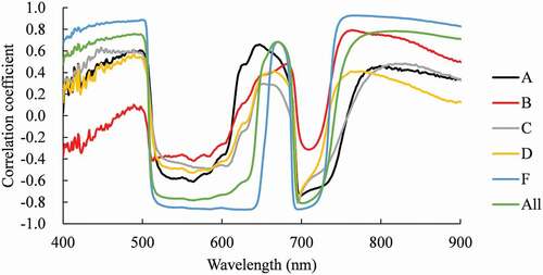
The correlation coefficients between chlorophyll content and reflectance after de-trending show two troughs (Figure 1), indicating high negative correlations near the green peak and the red edge inflection point (REIP). While these were most distinctive for treatment F, the lowest absolute values of correlation coefficients were recorded for treatment B. Although the significant positive correlations over the 400–500 nm range and wavelengths greater than 750 nm were identified for treatment F, these tendencies were not clear for other treatments. Furthermore, the positive correlations near 680 nm were identified for treatments A, B and F, however, the positions of their peaks differed. Positive correlations were not identified for treatments C and D.

Figure 1. Correlations between chlorophyll content and reflectance after de-trending. A: Enshi (horticultural experimental station) formula solution, B: two-thirds of solution, C: one third of solution, D: a sixth of solution, E: a twelfth of solution and F: no nitrogen treatment

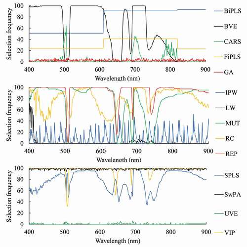
After one hundred repetitions, selected wavelengths selected by 14 PLS-based methods were shown in Figure 2. The average numbers of wavelengths selected by CARS, LW and UVE were less than 50, while those of BiPLS, RC, REP, SPLS, SwPA and VIP were more than 1000.

Figure 2. Frequency of each wavelength selected by different methods

Accuracy validation

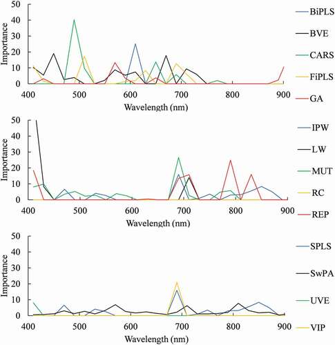
RPD and RMSE values were calculated using regression models based on machine learning algorithms using 100 iterations (Figure 3). The best combination of variable selection method and machine learning algorithm was REP and Cubist, achieving an RPD of 1.76 and an RMSE of 2.42 μg cm⁻². The importance at 20 nm interval as assessed by DSA and Cubist is shown in Figure 4. Generally, the high importance values were observed over REIP (680 to 720 nm) for all variable selection methods. Although some variable selection methods ignored the importance over the green peak, the highest importance was observed over it for CARS.

Figure 3. Relationships between ratio of performance to deviation (RPD) and root-mean-square error (RMSE) for different partial least square (PLS)-based variable selection methods for (a) Cubist, (b) DBN (deep belief nets), (c) RF (random forests), (d) SGB (stochastic gradient boosting) and (e) SVM (support vector machine)

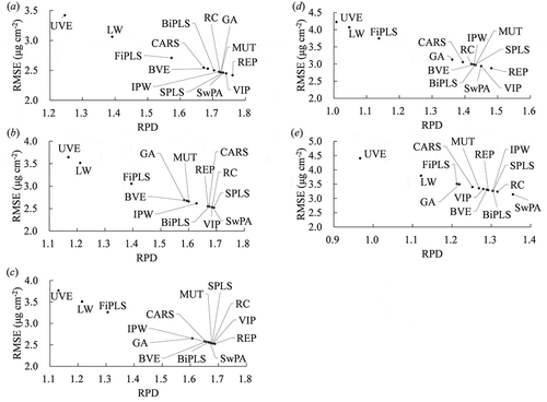
Figure 4. Relationships between selected wavelength and their importance based on DSA

Further, Cubist showed the best RPD values for all variable selection methods, while SVM was deemed unsuitable since its RPD values below 1.4 for all the selection methods investigated during this study. The RPD values of UVE, LW and FiPLS were also generally below 1.4, thus these methods are considered unsuitable for estimating chlorophyll content of muskmelon leaves using hyperspectral reflectance. In contrast, MUT, RC, REP, SPLS and SwPA showed potential with RPD values above 1.6.

Discussion

On 26 August, when the treatment was started, there were no significant differences among the six treatments. Within one to two weeks, the mean value of chlorophyll content became greater along with more nitrogen strength. A significant difference in chlorophyll content was confirmed between F and A, B, C and D on 2 September and between C and A, B, D and F and E and F on 9 September (p < 0.05, based on the Tukey–Kramer test).　Chlorophyll content became higher along with higher nitrogen strength, and that led to a lower reflectance, due to the strong absorption of chlorophyll-a and b under blue light (410–470 nm) and red light (644.8–670 nm), respectively (X. Chen et al., 2020; Navarro-Cerrillo et al., 2014).

Of the best combinations of variable selection methods and machine learning algorithms, both of REP and VIP, the most prominent variable selection methods, were selected 13 times after 100 repetitions each (Table 3). The high performances of VIP was also reported for estimating leaf chlorophyll content in winter wheat (He et al., 2015). SwPA (11 times), GA (9 times) and SPLS (8 times) were also effective as variable selection methods. These top five methods were selected 54 times in total. UVE, LW and FiPLS generally had RPD values below 1.4 when the measured values merged after 100 iterations (Figure 2). Previous studies reported a reduced performance of FiPLS, LW and UVE because these methods removed useful information (Santos-Rufo et al., 2020; Xia et al., 2017). The reflectance at 550 nm, which is frequently noted as the green peak, was applied for estimating chlorophyll content in some studies (Carter & Knapp, 2001; Datt, 1998). Indeed, the green peak becomes tiny with higher chlorophyll content. However, some studies have reported that chlorophyll contributes to reflectance at 550 nm especially for low anthocyanin content against a high background of chlorophyll (Merzlyak et al., 2003). Besides the green peak, the red edge has also been used for chlorophyll content estimation and is shifted to longer wavelengths with higher chlorophyll content (Gitelson & Solovchenko, 2017; Miller et al., 1990). The performance of FiPLS, LW and UVE relied on the red edge, and sometimes the wavelengths over the green peaks were removed at 100 repetitions. In contrast, the other methods utilised both the green peak and red edge. Ram et al. (2011) reported that anthocyanin induction was strongly influenced by low nitrogen concentration. The effects of anthocyanin differ in reflectance at the green peak and red edge: at the red edge chlorophyll does absorb but anthocyanin does not, whereas the absorption of anthocyanin is at maximum at the green peak (Gitelson et al., 2006). Using the green peak might therefore introduce inaccuracies related to senescence or stress caused by lack of nitrogen.

Table 3. Best combinations of variable selection methods and machine learning algorithms after 100 repetitions

Variable selection method	Machine learning algorithm	Time	Variable selection method	Machine learning algorithm	Time
BiPLS	Cubist	2	RC	Cubist	1
BiPLS	DBN	3	RC	DBN	3
BiPLS	RF	1	RC	SVM	1
BiPLS	SVM	1	REP	Cubist	3
BVE	Cubist	4	REP	DBN	4
BVE	RF	1	REP	RF	1
BVE	SGB	2	REP	SGB	3
CARS	Cubist	1	REP	SVM	2
CARS	DBN	2	SPLS	Cubist	5
CARS	RF	1	SPLS	DBN	2
CARS	SVM	1	SPLS	SVM	1
FiPLS	Cubist	2	SwPA	Cubist	6
FiPLS	DBN	1	SwPA	DBN	3
FiPLS	SGB	1	SwPA	RF	1
GA	Cubist	3	SwPA	SVM	1
GA	DBN	5	UVE	Cubist	2
GA	SGB	1	UVE	SGB	2
IPW	Cubist	2	UVE	SVM	1
IPW	DBN	2	VIP	Cubist	2
IPW	RF	1	VIP	DBN	7
IPW	SGB	1	VIP	RF	1
LW	Cubist	1	VIP	SVM	3
MUT	Cubist	4
MUT	SVM	2

The RPD values of the regression models based on UVE and LW were less than 1.4, which meant that they were not suitable valuable selection methods. The average numbers of wavelengths selected by UVE and LW were 10, which was the smallest value. Some previous studies (Santos-Rufo et al., 2020; Xia et al., 2017) reported they greatly reduce variables but also remove some useful information and then this characteristic was confirmed in this study.

The machine learning algorithms Cubist (38 times) and DBN (32 times) were generally selected. Potential methods for using with these algorithms were SwPA (6 and 3 times for Cubist and DBN, respectively), GA (3 and 5 times), REP (3 and 4 times), SPLS (5 and 2 times) and VIP (2 and 7 times). For kernel-based algorithms, an inappropriate selection of hyperparameters relates to kernel function (Horvath, 2003), and so different ranges of kernel-related parameters for SVM have been suggested: from 0.005 (Foody & Mathur, 2004) to 2⁸ (Sonobe et al., 2014), although greater values may lead to a decrease in accuracy by more than 20% (Trisasongko, 2017). In the present study, σ ranged from 2⁻²¹ to 2⁵⁰ with a mode of 2° (7 times per 100 iterations), but no generally preferable value could be determined. Kp ranged from 2⁻⁷ to 2° with a mode of 2⁻⁵ (24 times per 100 iterations). Although Cubist, RF and SGB are all stochastic modelling techniques involving ensemble regression trees or rule-based models, the performances of RF and SGB were obviously lower than that of Cubist. Cubist’s proficiency has been demonstrated by comparing 77 popular regression methods (Fernandez-Delgado et al., 2019). SGB fails if the training data set is small, and since only a fraction of the training data was sampled in this algorithm (n = 100 in this study), overfitting was likely. When running RF (“randomForest” package; (Breiman et al., 2018)), one third of the training data is separated as out-of-bag (OOB) samples. These data are not considered in the training of the tree and can be used to evaluate performance. However, this strategy might have reduced sample size too much to generate regression models, as RF did not perform as well as in previous studies (Biau & Scornet, 2016). A lot of earlier studies have reported the best machine learning algorithms for estimating leaf chlorophyll contents from hyperspectral reflectance or vegetation indices calculated from reflectance (An et al., 2020; Zhu et al., 2020), however, the combinations of machine learning algorithms and wavelength selection methods were not conducted. The results indicated wavelengths selection is a critical step for chlorophyll content estimation and suitable selection methods made estimation accuracies higher.

In order to evaluate whether the proposed method was effective to the other species, ANGERS (Feret et al., 2008), which includes the measurements from 41 different species and is the dataset measured in 2003 at INRA in Angers (France), were used for validations. Figure 5 shows the relationships between measured and estimated values. Although the estimated values were constant for the samples whose chlorophyll contents were bigger than 60 μg cm⁻² or smaller than 10 μg cm⁻² (these values were not included the measurements from the muskmelon leaves), the proposed method still had the high performance with a root mean square error of 11.30 μg cm⁻² with RPD values of 1.92.

Figure 5. Relationship between measured and estimated chlorophyll contents

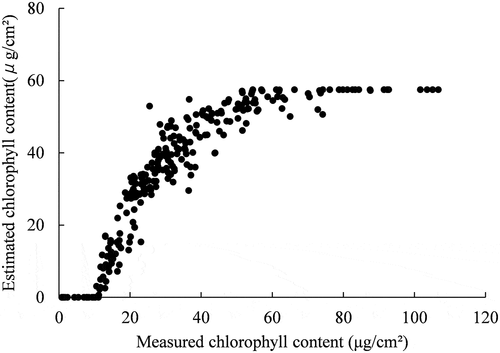
In this study, six nitrogen treatments were applied to produce various causes related to the chlorophyll contents and then reflectance of muskmelon leaves in a wide range of chlorophyll content was investigated in this study. However, ANGERS is larger dataset and includes leaves with very low pigment contents, and sometimes, with almost no carotenoids or no chlorophylls (Feret et al., 2008). Especially, the lower and higher chlorophyll contents were confirmed in the measurements from broad leaf trees. Broad leaf trees generally have two distinctive leaf types including shaded and sunlit leaves. Sunlit leaves were grown under high irradiances and are much less susceptible to photoinhibitory damage than shaded leaves (Powles, 1984), while shaded leaves are commonly larger and thinner than sunlit leaves (Terashima et al., 2001). The difference between the two types of leaves in broad-leaved trees should be linked to the chlorophyll content estimation models to improve the accuracy for the measurements from broad leaf trees.

Leaf scale spectroscopy is effective to confirm direct links of reflected information with chlorophyll content, since surrounding effects would have been under controlled. Some variable selection algorithms have been proposed to assess chlorophyll contents from canopy spectra (H.J. Liu et al., 2019; N. Liu et al., 2020; Yang et al., 2021) and satellite- or air-borne remote-sensing data are more of professional applications concerning large scale assessment and then their potentials should be assessed in the future works.

Conclusions

Dimension reduction strategy is important for eliminating redundant and irrelevant features and improving accuracy of estimations of vegetation properties using hyperspectral reflectance. To this end, the use of PLS-based feature selection methods has been proposed. However, the influences of the feature selection methods and machine learning algorithms were unknown. Therefore, combinations of 14 PLS-based variable selection methods and 5 common machine learning algorithms were evaluated for their potential for estimating chlorophyll content of muskmelon leaves using hyperspectral reflectance.

Generally, Cubist and DBN performed well for this purpose. Algorithms were more important for evaluating chlorophyll content, however, improvements were identified for combinations with one of five PLS-based variable selection methods: SwPA, GA, REP, SPLS and VIP. These methods can be considered effective for enabling precise agricultural analyses in this context.

Although de-trending was used to pre-process reflectance data in this study, vegetation indices are also effective for removing noise and reducing the data saturation problem. Therefore, it would be beneficial to test the efficacy of vegetation indices for further improving chlorophyll content monitoring.

Disclosure statement

No potential conflict of interest was reported by the author(s).

Additional information

Funding

This study was supported financially by JSPS KAKENHI [grant number 19K06313].

References

- An, G. Q., Xing, M. F., He, B. B., Liao, C. H., Huang, X. D., Shang, J. L., & Kang, H. Q. (2020). Using Machine Learning for Estimating Rice Chlorophyll Content from In Situ Hyperspectral Data. Remote Sensing, 12(18), 20. https://doi.org/https://doi.org/10.3390/rs12183104
- Balabin, R. M., & Smirnov, S. V. (2011). Variable selection in near-infrared spectroscopy: Benchmarking of feature selection methods on biodiesel data. Analytica Chimica Acta, 692(1–2), 63–72. https://doi.org/https://doi.org/10.1016/j.aca.2011.03.006
- Barnes, R. J., Dhanoa, M. S., & Lister, S. J. (1989). Standard Normal Variate Transformation and De-Trending of Near-Infrared Diffuse Reflectance Spectra. Applied Spectroscopy, 43(5), 772–777. https://doi.org/https://doi.org/10.1366/0003702894202201
- Biau, G., & Scornet, E. (2016). A random forest guided tour. Test, 25(2), 197–227. https://doi.org/https://doi.org/10.1007/s11749-016-0481-7
- Breiman, L. (2001). Random forests. Machine Learning, 45(1), 5–32. https://doi.org/https://doi.org/10.1023/A:1010933404324
- Breiman, L., Cutler, A., Liaw, A., & Wiener, M., 2018. Breiman and Cutler’s Random Forests for Classification and Regression [online]. Retrieved January 5, 2021, from https://cran.r-project.org/web/packages/randomForest/randomForest.pdf
- Breunig, F. M., Galvao, L. S., Dalagnol, R., Dauve, C. E., Parraga, A., Santi, A. L., Della Flora, D. P., & Chen, S. S. (2020). Delineation of management zones in agricultural fields using cover crop biomass estimates from PlanetScope data. International Journal of Applied Earth Observation and Geoinformation, 85, 102004. https://doi.org/https://doi.org/10.1016/j.jag.2019.102004
- Burges, C. J. C. (1998). A tutorial on Support Vector Machines for pattern recognition. Data Mining and Knowledge Discovery, 2(2), 121–167. https://doi.org/https://doi.org/10.1023/A:1009715923555
- Candolfi, A., De Maesschalck, R., Jouan-Rimbaud, D., Hailey, P. A., & Massart, D. L. (1999). The influence of data pre-processing in the pattern recognition of excipients near-infrared spectra. Journal of Pharmaceutical and Biomedical Analysis, 21(1), 115–132. https://doi.org/https://doi.org/10.1016/S0731-7085(99)00125-9
- Carter, G. A., & Knapp, A. K. (2001). Leaf optical properties in higher plants: Linking spectral characteristics to stress and chlorophyll concentration. American Journal of Botany, 88(4), 677–684. https://doi.org/https://doi.org/10.2307/2657068
- Chang, C. C., Chien, L. J., & Lee, Y. J. (2011). A novel framework for multi-class classification via ternary smooth support vector machine. Pattern Recognition, 44(6), 1235–1244. https://doi.org/https://doi.org/10.1016/j.patcog.2010.11.016
- Chang, C. W., Laird, D. A., Mausbach, M. J., & Hurburgh, C. R. (2001). Near-infrared reflectance spectroscopy-principal components regression analyses of soil properties. Soil Science Society of America Journal, 65(2), 480–490. https://doi.org/https://doi.org/10.2136/sssaj2001.652480x
- Chen, N. L., Tang, R. Y., Zhang, Y. X., An, C. X., & Gao, H. J. (2010). Photosynthetic and Biochemical Changes of Melon Leaves during Senescence. Iv International Symposium on Cucurbits, 871, 329–336. https://doi.org/https://doi.org/10.17660/ActaHortic.2010.871.45
- Chen, X., Dong, Z., Liu, J., Wang, H., Zhang, Y., Chen, T., Du, Y., Shao, L., & Xie, J. (2020). Hyperspectral characteristics and quantitative analysis of leaf chlorophyll by reflectance spectroscopy based on a genetic algorithm in combination with partial least squares regression. Spectrochimica Acta Part A: Molecular and Biomolecular Spectroscopy, 243, 118786. https://doi.org/https://doi.org/10.1016/j.saa.2020.118786
- Chong, I. G., & Jun, C. H. (2005). Performance of some variable selection methods when multicollinearity is present. Chemometrics and Intelligent Laboratory Systems, 78(1–2), 103–112. https://doi.org/https://doi.org/10.1016/j.chemolab.2004.12.011
- Cortez, P., & Embrechts, M. J. (2013). Using sensitivity analysis and visualization techniques to open black box data mining models. Information Sciences, 225(10), 1–17. https://doi.org/https://doi.org/10.1016/j.ins.2012.10.039
- Datt, B. (1998). Remote sensing of chlorophyll a, chlorophyll b, chlorophyll a+b, and total carotenoid content in eucalyptus leaves. Remote Sensing of Environment, 66(2), 111–121. https://doi.org/https://doi.org/10.1016/S0034-4257(98)00046-7
- Datt, B. (1999). Visible/near infrared reflectance and chlorophyll content in Eucalyptus leaves. International Journal of Remote Sensing, 20(14), 2741–2759. https://doi.org/https://doi.org/10.1080/014311699211778
- Fan, S. X., Zhang, B. H., Li, J. B., Huang, W. Q., & Wang, C. P. (2016). Effect of spectrum measurement position variation on the robustness of NIR spectroscopy models for soluble solids content of apple. Biosystems Engineering, 143, 9–19. https://doi.org/https://doi.org/10.1016/j.biosystemseng.2015.12.012
- Feret, J. B., Francois, C., Asner, G. P., Gitelson, A. A., Martin, R. E., Bidel, L. P. R., Ustin, S. L., Le Maire, G., & Jacquemoud, S. (2008). PROSPECT-4 and 5: Advances in the leaf optical properties model separating photosynthetic pigments. Remote Sensing of Environment, 112(6), 3030–3043. https://doi.org/https://doi.org/10.1016/j.rse.2008.02.012
- Fernandez-Delgado, M., Sirsat, M. S., Cernadas, E., Alawadi, S., Barro, S., & Febrero-Bande, M. (2019). An extensive experimental survey of regression methods. Neural Networks, 111, 11–34. https://doi.org/https://doi.org/10.1016/j.neunet.2018.12.010
- Foody, G. M., & Mathur, A. (2004). A relative evaluation of multiclass image classification by support vector machines. IEEE Transactions on Geoscience and Remote Sensing, 42(6), 1335–1343. https://doi.org/https://doi.org/10.1109/TGRS.2004.827257
- Forina, M., Casolino, C., & Millan, C. P. (1999). Iterative predictor weighting (IPW) PLS: A technique for the elimination of useless predictors in regression problems. Journal of Chemometrics, 13(2), 165–184. https://doi.org/https://doi.org/10.1002/(SICI)1099-128X(199903/04)13:2<165::AID-CEM535>3.0.CO;2-Y
- Friedman, J. H. (2002). Stochastic gradient boosting. Computational Statistics & Data Analysis, 38(4), 367–378. https://doi.org/https://doi.org/10.1016/S0167-9473(01)00065-2
- Gitelson, A., & Solovchenko, A. (2017). Generic Algorithms for Estimating Foliar Pigment Content. Geophysical Research Letters, 44(18), 9293–9298. https://doi.org/https://doi.org/10.1002/2017GL074799
- Gitelson, A. A., Keydan, G. P., & Merzlyak, M. N. (2006). Three-band model for noninvasive estimation of chlorophyll, carotenoids, and anthocyanin contents in higher plant leaves. Geophysical Research Letters, 33(11). https://doi.org/https://doi.org/10.1029/2006GL026457
- Golhani, K., Balasundram, S. K., Vadamalai, G., & Pradhan, B. (2019). Estimating chlorophyll content at leaf scale in viroid-inoculated oil palm seedlings (Elaeis guineensis Jacq.) using reflectance spectra (400 nm-1050 nm). International Journal of Remote Sensing, 40(19), 7647–7662. https://doi.org/https://doi.org/10.1080/01431161.2019.1584930
- Hastie, T., Tibshirani, R., & Friedman, J. (2009). The Elements of Statistical Learning: Data Mining, Inference, and Prediction; (2nd ed.). Springer.
- He, P., Xu, X. G., Zhang, B. L., Li, Z. H., Feng, H. K., Yang, G. J., & Zhang, Y. F., 2015. Estimation of leaf chlorophyll content in winter wheat using variable importance for projection (VIP) with hyperspectral dataed. Conference on Remote Sensing for Agriculture, Ecosystems, and Hydrology XVII part of the International Symposium on Remote Sensing, Toulouse, France: SPIE.
- Hinton, G. E., Osindero, S., & Teh, Y. W. (2006). A fast learning algorithm for deep belief nets. Neural Computation, 18, 1527–1554. https://doi.org/https://doi.org/10.1162/neco.2006.18.7.1527
- Horvath, G., 2003. CMAC neural network as an SVM with B-spline kernel functionsed. 20th IEEE Instrumentation and Measurement Technology Conference, Vail, CO, 1108–1113. IEEE.
- Kewley, R. H., Embrechts, M. J., & Breneman, C. (2000). Data strip mining for the virtual design of pharmaceuticals with neural networks. IEEE Transactions on Neural Networks, 11(3), 668–679. https://doi.org/https://doi.org/10.1109/72.846738
- Le Cao, K. A., Rossouw, D., Robert-Granie, C., & Besse, P. (2008). A Sparse PLS for Variable Selection when Integrating Omics Data. Statistical Applications in Genetics and Molecular Biology, 7(1). https://doi.org/https://doi.org/10.2202/1544-6115.1390
- Li, H. D., Zeng, M. M., Tan, B. B., Liang, Y. Z., Xu, Q. S., & Cao, D. S. (2010). Recipe for revealing informative metabolites based on model population analysis. Metabolomics, 6(3), 353–361. https://doi.org/https://doi.org/10.1007/s11306-010-0213-z
- Lindgren, F., Geladi, P., Rannar, S., & Wold, S. (1994). Interactive variable selection (IVS) for pls. Part 1: Theory and algorithms. Journal of Chemometrics, 8(5), 349–363. https://doi.org/https://doi.org/10.1002/cem.1180080505
- Liu, H. J., Li, M. Z., Zhang, J. Y., Gao, D. H., Sun, H., Zhang, M., & Wu, J. Z. (2019). A novel wavelength selection strategy for chlorophyll prediction by MWPLS and GA. International Journal of Agricultural and Biological Engineering, 12(5), 149–155. https://doi.org/https://doi.org/10.25165/j.ijabe.20191205.4033
- Liu, N., Qiao, L., Xing, Z. Z., Li, M. Z., Sun, H., Zhang, J. Y., & Zhang, Y. (2020). Detection of chlorophyll content in growth potato based on spectral variable analysis. Spectroscopy Letters, 53(6), 476–488. https://doi.org/https://doi.org/10.1080/00387010.2020.1772827
- Lu, B., Dao, P. D., Liu, J. G., He, Y. H., & Shang, J. L. (2020). Recent Advances of Hyperspectral Imaging Technology and Applications in Agriculture. Remote Sensing, 12(16), 44. https://doi.org/https://doi.org/10.3390/rs12162659
- Mehmood, T., Liland, K. H., Snipen, L., & Saebo, S. (2012). A review of variable selection methods in Partial Least Squares Regression. Chemometrics and Intelligent Laboratory Systems, 118(15), 62–69. https://doi.org/https://doi.org/10.1016/j.chemolab.2012.07.010
- Merzlyak, M. N., Solovchenko, A. E., & Gitelson, A. A. (2003). Reflectance spectral features and non-destructive estimation of chlorophyll, carotenoid and anthocyanin content in apple fruit. Postharvest Biology and Technology, 27(2), 197–211. https://doi.org/https://doi.org/10.1016/S0925-5214(02)00066-2
- Miller, J. R., Hare, E. W., & Wu, J. (1990). Quantitative characterisation of the red edge reflectance 1. An inverted-Gaussian model. International Journal of Remote Sensing, 11(10), 1755–1773. https://doi.org/https://doi.org/10.1080/01431169008955128
- Navarro-Cerrillo, R. M., Trujillo, J., De La Orden, M. S., & Hernandez-Clemente, R. (2014). Hyperspectral and multispectral satellite sensors for mapping chlorophyll content in a Mediterranean Pinus sylvestris L. plantation. International Journal of Applied Earth Observation and Geoinformation, 26, 88–96. https://doi.org/https://doi.org/10.1016/j.jag.2013.06.001
- Pan, L. Q., Lu, R. F., Zhu, Q. B., Tu, K., & Cen, H. Y. (2016). Predict Compositions and Mechanical Properties of Sugar Beet Using Hyperspectral Scattering. Food and Bioprocess Technology, 9(7), 1177–1186. https://doi.org/https://doi.org/10.1007/s11947-016-1710-5
- Pierna, J. A. F., Abbas, O., Baeten, V., & Dardenne, P. (2009). A Backward Variable Selection method for PLS regression (BVSPLS). Analytica Chimica Acta, 642(1–2), 89–93. https://doi.org/https://doi.org/10.1016/j.aca.2008.12.002
- Powles, S. B. (1984). Photoinhibition of Photosynthesis Induced by Visible Light. Annual Review of Plant Physiology, 35(1), 15–44. https://doi.org/https://doi.org/10.1146/annurev.pp.35.060184.000311
- Quinlan, J. R., 1992. Learning with Continuous Classe.ed.^eds. 5th Australian Joint Conference on Artificial Intelligence, Hobart, TAS, World Scientific: Australia, 343–348.
- Ram, M., Prasad, K.V., Kaur, C., Singh, S.K., Arora, A. & Kumar, S., 2011. Induction of anthocyanin pigments in callus cultures of Rosa hybrida L. in response to sucrose and ammonical nitrogen levels. Plant Cell Tissue and Organ Culture, 104 (2), 171–179
- Romeo, L., Loncarski, J., Paolanti, M., Bocchini, G., Mancini, A., & Frontoni, E. (2020). Machine learning-based design support system for the prediction of heterogeneous machine parameters in industry 4.0. Expert Systems with Applications, 140, 112869. https://doi.org/https://doi.org/10.1016/j.eswa.2019.112869
- Samat, A., Liu, S. C., Persello, C., Li, E. Z., Miao, Z. L., & Abuduwaili, J. (2019). Evaluation of ForestPA for VHR RS image classification using spectral and superpixel-guided morphological profiles. European Journal of Remote Sensing, 52(1), 107–121. https://doi.org/https://doi.org/10.1080/22797254.2019.1565418
- Santos-Rufo, A., Mesas-Carrascosa, F. J., Garcia-Ferrer, A., & Merono-Larriva, J. E. (2020). Wavelength Selection Method Based on Partial Least Square from Hyperspectral Unmanned Aerial Vehicle Orthomosaic of Irrigated Olive Orchards. Remote Sensing, 12(20), 3426. https://doi.org/https://doi.org/10.3390/rs12203426
- Sonobe, R., Miura, Y., Sano, T., & Horie, H. (2018). Monitoring Photosynthetic Pigments of Shade-Grown Tea from Hyperspectral Reflectance. Canadian Journal of Remote Sensing, 44(2), 104–112. https://doi.org/https://doi.org/10.1080/07038992.2018.1461555
- Sonobe, R., Tani, H., Wang, X. F., Kobayashi, N., & Shimamura, H. (2014). Parameter tuning in the support vector machine and random forest and their performances in cross- and same-year crop classification using TerraSAR-X. International Journal of Remote Sensing, 35(23), 7898–7909. https://doi.org/https://doi.org/10.1080/01431161.2014.978038
- Sonobe, R., Yamashita, H., Mihara, H., Morita, A., & Ikka, T. (2020). Estimation of Leaf Chlorophyll a, b and Carotenoid Contents and Their Ratios Using Hyperspectral Reflectance. Remote Sensing, 12(19), 3265. https://doi.org/https://doi.org/10.3390/rs12193265
- Sonobe, R., Yamashita, H., Nofrizal, A. Y., Seki, H., Morita, A., & Takashi, I. (2021). Use of spectral reflectance from a compact spectrometer to assess chlorophyll content in Zizania latifolia. Geocarto International, 1914747. https://doi.org/https://doi.org/10.1080/10106049.2021.1914747
- Srivastava, N., Hinton, G., Krizhevsky, A., Sutskever, I., & Salakhutdinov, R. (2014). Dropout: A Simple Way to Prevent Neural Networks from Overfitting. Journal of Machine Learning Research, 15(1), 1929–1958. https://www.jmlr.org/papers/volume15/srivastava14a/srivastava14a.pdf
- Sugiyama, K., Matsuno, K., Doi, M., Tatara, A., Kato, M., & Tagam, Y. (2008). TYLCV detection in Bemisia tabaci (Gennadius) (Hemiptera: Aleyrodidae) B and Q biotypes, and leaf curl symptom of tomato and other crops in winter greenhouses in Shizuoka Pref., Japan. Applied Entomology and Zoology, 43(4), 593–598. https://doi.org/https://doi.org/10.1303/aez.2008.593
- Terashima, I., & Hikosaka, K. (1995). Comparative ecophysiology of leaf and canopy photosynthesis. Plant, Cell & Environment, 18(10), 1111–1128. https://doi.org/https://doi.org/10.1111/j.1365-3040.1995.tb00623.x
- Terashima, I., Miyazawa, S. I., & Hanba, Y. T. (2001). Why are Sun Leaves Thicker than Shade Leaves? — Consideration based on Analyses of CO2 Diffusion in the Leaf. Journal of Plant Research, 114(1), 93–105. https://doi.org/https://doi.org/10.1007/PL00013972
- Trisasongko, B. H. (2017). Mapping stand age of rubber plantation using ALOS-2 polarimetric SAR data. European Journal of Remote Sensing, 50(1), 64–76. https://doi.org/https://doi.org/10.1080/22797254.2017.1274569
- Uddin, M. Z., Hassan, M. M., Alsanad, A., & Savaglio, C. (2020). A body sensor data fusion and deep recurrent neural network-based behavior recognition approach for robust healthcare. Information Fusion, 55, 105–115. https://doi.org/https://doi.org/10.1016/j.inffus.2019.08.004
- Villar, A., Fernandez, S., Gorritxategi, E., Ciria, J. I., & Fernandez, L. A. (2014). Optimization of the multivariate calibration of a Vis-NIR sensor for the on-line monitoring of marine diesel engine lubricating oil by variable selection methods. Chemometrics and Intelligent Laboratory Systems, 130(15), 68–75. https://doi.org/https://doi.org/10.1016/j.chemolab.2013.10.008
- Wang, W. J., Xu, Z. B., Lu, W. Z., & Zhang, X. Y. (2003). Determination of the spread parameter in the Gaussian kernel for classification and regression. Neurocomputing, 55(3–4), 643–663. https://doi.org/https://doi.org/10.1016/S0925-2312(02)00632-X
- Wang, Y. G., Gao, Y., Yu, X. Z., Wang, Y. Y., Deng, S., & Gao, J. M. (2016). Rapid Determination of Lycium Barbarum Polysaccharide with Effective Wavelength Selection Using Near-Infrared Diffuse Reflectance Spectroscopy. Food Analytical Methods, 9(1), 131–138. https://doi.org/https://doi.org/10.1007/s12161-015-0178-7
- Wellburn, A. R. (1994). The spectral determination of chlorophyll a and chlorophyll b, as well as total carotenoids, using various solvents with spectrophotometers of different resolution. Journal of Plant Physiology, 144(3), 307–313. https://doi.org/https://doi.org/10.1016/S0176-1617(11)81192-2
- Williams, P., & Norris, K. (1987). Near- Infrared Technology in the Agricultural and Food Industries. American Association of Cereal Chemists Inc.
- Xia, Z. Y., Zhang, C., Weng, H. Y., Nie, P. C., & He, Y. (2017). Sensitive Wavelengths Selection in Identification of Ophiopogon japonicus Based on Near-Infrared Hyperspectral Imaging Technology. International Journal of Analytical Chemistry, 2017, 1–11. https://doi.org/https://doi.org/10.1155/2017/6018769
- Xie, R., Darvishzadeh, R., Skidmore, A. K., Heurich, M., Holzwarth, S., Gara, T. W., & Reusen, I. (2021). Mapping leaf area index in a mixed temperate forest using Fenix airborne hyperspectral data and Gaussian processes regression. International Journal of Applied Earth Observation and Geoinformation, 95, 102242. https://doi.org/https://doi.org/10.1016/j.jag.2020.102242
- Yang, J., Yang, S. X., Zhang, Y. Y., Shi, S., & Du, L. (2021). Improving characteristic band selection in leaf biochemical property estimation considering interrelations among biochemical parameters based on the PROSPECT-D model. Optics Express, 29(1), 400–414. https://doi.org/https://doi.org/10.1364/OE.414050
- Zhu, W. X., Sun, Z. G., Yang, T., Li, J., Peng, J. B., Zhu, K. Y., Li, S. J., Gong, H. R., Lyu, Y., Li, B. B., & Liao, X. H. (2020). Estimating leaf chlorophyll content of crops via optimal unmanned aerial vehicle hyperspectral data at multi-scales. Computers and Electronics in Agriculture, 178, 16. https://doi.org/https://doi.org/10.1016/j.compag.2020.105786