A novel method for predicting the geochemical composition of tailings with laboratory field and hyperspectral airborne data using a regression and classification-based approach

ABSTRACT

The increasing demand for precise and dependable models has led to the development of both sensors and statistical algorithms. However, numerous studies have demonstrated that model performance is highly dependent on a range of environmental factors, such as spatio-temporal fluctuations of moisture, sensor type, sample variability, preprocessing methods, and model selection. These factors can impact prediction results, leading to erroneous comparisons across lab, field, or imaging models. Samples for this study were collected from a tailing settling basin of a porphyry copper deposit near Erdenet, Mongolia. The database contains lab and field spectra and hyperspectral imagery from a HySpex imaging sensor. In this study we propose a workflow that includes a simulation that yields an appropriate regression threshold while addressing data-driven uncertainty. The workflow consists of two regression models and five classification models at different scales for quantitative geochemical, mineralogical, and textural prediction of tailing samples. Each model is compared to the acquisition space's performance potential. Acceptable R² values for regression models are 0.58 for laboratory, 0.40 for field, and 0.31 for hyperspectral airborne data. Results of this study are not limited to tailing samples but can be applied on other fields of research such as geology, pedology or agriculture.

KEYWORDS:

• tailing
• regression
• classification
• hyperspectral remote sensing
• geochemistry
• spectroscopy

Introduction

The balance between accurate prediction, processing speed and calibration efforts is the key challenge to the success of any model which is based on either point spectroscopy or imaging spectroscopy. In recent years, with the development of high-resolution sensors (spatial and spectral) on the one hand, and high processing capabilities on the other hand, high accuracy levels can be aspired to and achieved quickly and efficiently. Laboratory, field, and imaging measurements have been proven to be useful tools for geochemical assessment (Clark, 1999; Clark et al., 2006; Mishra et al., 2021; Rowan & Mars, 2003; Thiele et al., 2021; Van der Meer, 2018). Many studies investigated the capabilities of hyperspectral data for monitoring the geochemical, mineralogical and textural properties of natural resources such as in soils and rocks (Awad et al., 2018; Cudahy et al., 2001; Dkhala et al., 2020; Feng et al., 2018; Gomez et al., 2008; King et al., 2004; J. Liu et al., 2021a; Mendes et al., 2021; Murphy & Monteiro, 2013; Son et al., 2021), but also of anthropogenic activity which causes an accumulation of minerals for example, in tailings and other mining activities (Hao et al., 2019; Khajehzadeh et al., 2017; Purwadi et al., 2020; Shang et al., 2009).

Estimating heavy metal such as Cu, Fe, Al, and Zn have been the main objective in many studies (Pandit et al., 2010; Ren et al., 2009; Tan et al., 2021; Wang et al., 2017; Wu et al., 2011), however, it is not limited only to natural soils but also to tailing materials (Pyo et al., 2020). Several transition metals including Cu, can present spectral features (610 and 830 nm) in the VNIR spectra of soil samples under two conditions: (i) they exhibit very high concentrations (>4000 mg kg⁻¹) and (ii) they have an unfilled d shell (Wu et al., 2007).

Tailings, which are part of the mining residues, may contain a large amount of valuable minerals such as various metals. Tailing material can be comparable to soil by their similar textural parameters (clay-silt-sand ratio) and to rocks by their geochemical composition. However, unlike soils, tailings do not contain organic matter and do not exhibit the long-term natural horizon development, although heavy metal migration does take place in space (Myagkaya et al., 2010). A recent study by Suppes and Heuss-Aßbichler (2021) has defined tailings as an anthropogenic raw material and recommended to investigate the important question whether mineral and structure-related information on tailing storage facilities can be obtained with remote sensing data.

In recent years, many studies have focused on tailings to monitor and map heavy metals (Brown et al., 1999; Munir et al., 2021), the mineralogical composition (Dkhala et al., 2020; Khajehzadeh et al., 2017; Moncur et al., 2005; Shang et al., 2009), and water retention (Aubertin et al., 1998). However, although conducting a research in an active tailing facility is a challenging task due to a lack of accessibility and high water content, the relatively homogenous geochemical composition which is reflected in the spectral data can facilitate the spectral analysis and improve model prediction (Moura-Bueno et al., 2019; Ogen et al., 2019a).

An upscaling approach for geochemical prediction has been examined by (Dkhala et al., 2020) using field measurements of dry and undisturbed samples, Sentinel-2 data (www.sentinel.esa.int) and simulated Sentinel-2 data extracted from the field measurements. The highest prediction was obtained for quartz with R² = 0.73. Their results show a satisfying prediction (for four of the seven studied minerals) using field spectra covering the visible light, near infrared and shortwave infrared (VNIR-SWIR), a slight decrease in performance for the simulated Sentinel-2 data but encountered a significant decrease of performances for six out of seven minerals when using Sentinel-2 data.

Chemometric models based on spectral measurements conducted in supervised laboratory conditions have the advantage of being more accurate than other acquisition methods (field and airborne data) which are influenced by unstable environmental conditions. However, both demand intensive field work (Fenstermaker & Mlller, 1994). On the other hand, hyperspectral remote sensing is subjected to precise calibrations, geometric and topographic conditions, and the influence of the atmosphere (Ben‐Dor et al., 2008). Therefore, it may provide prediction models that are less accurate. However, it can survey large and inaccessible areas and offer a cost-effective way to collect and process the spectral data (Shang et al., 2009). Stevens et al. (2008) examined the models’ performance when applied to laboratory, field, and airborne spectroscopy. They found that despite its better potential for covering broad areas, airborne data poses certain challenges for model prediction due to a lower Signal-to-Noise Ratio (SNR). Moreover, they concluded that the accuracy of field measurements is equivalent to laboratory measurements, only when it is performed under specific surface conditions (low variation in moisture and low roughness).

In addition to that, other various factors can influence the model’s performance and accuracy such as sample size, data variability, analyte concentration, water/moisture content, surface roughness, spectral features, and data preprocessing. For instance, a limited number of training samples can affect the performance of prediction models (Ng et al., 2020) or inhibit the performance of classification models (Wambugu et al., 2021), data with low variability (lower than the measurement error) cannot contain enough information about the parameter in question (Forina et al., 2000), and a low concentration of the analyte or even below the detection limit of the spectral sensor may affect the reliability of the models (DiFoggio, 2000; Ogen et al., 2018). In addition, water content may change the spectral fingerprint and blur significant absorption features caused by major chromophores and thus affect the models (Clark, 1999; Ogen et al., 2019b), surface roughness may lower the reflectance values due to micro shading (Stevens et al., 2008), a lack of diagnostic spectral features for felsic minerals (e.g. feldspars and quartz) occurs in the VNIR-SWIR regions in contrast to their presence in the longwave infrared (LWIR) region (Feng et al., 2018), the presence of unknown classes that may exist in the image (S. Liu et al., 2021b), and different preprocessing approaches have serious drawbacks when transforming the data and may provide misleading results that can even sum up to more than 20% difference in model accuracy (Engel et al., 2013). Furthermore, international round robin tests highlight the variations and errors due to instruments, measurement protocols, and sample handling that can occur at the laboratory scale (Götze et al., 2017; Langsdale et al., 2021).

Steinberg et al. (2016) compared the prediction of iron oxides, clay, and organic matter using the Hyperspectral Mapper (HyMap) and the Airborne Hyperspectral system (AHS) (R² between 0.64 and 0.74) and simulated EnMap satellite imagery (R² between 0.53 and 0.67). In addition, they concluded that uncertainties in the spectral data due to the atmosphere, surface roughness, sensor noise and illumination can be responsible to 70–80% of the variance of their results. On the contrary, Gomez et al. (2015) found that the atmosphere appears to only slightly affect the performance of regression-based models. However, their study was conducted in optimal atmospheric conditions (very low content of water vapor) and with higher concentration and variability of clay which ranged between 108 and 772 g kg⁻¹ (equivalent to 10.8–77.2%).

The possibility of errors which may influence the uncertainty increases when spectral measurements are made in a variety of environmental conditions (laboratory, field, and airborne) and few studies have confronted this issue by quantifying the uncertainties of the spectral data (Carmon et al., 2020; Jiménez et al., 2018; Thompson et al., 2020). Stein et al. (2009) presented a summary of four sources that can cause errors: the pixel, the objects, monitoring, and prediction. Lagacherie et al. (2008) showed that the main source of uncertainty when scaling up laboratory to airborne observations is the ability of airborne reflectance data to be spectrally consistent and properly adjusted for atmospheric variables, particularly water vapor. These effects degrade the quality of data as it shifts from laboratory to field measurements and then to imaging data. In addition to that, Carmon et al. (2020) confirmed that iron oxides are much more sensitive to the atmosphere compared with alteration minerals. Moreover, Jiménez et al. (2018) found that due to various factors such as the equipment performance, measurement methodology, sampling strategy, surface properties, and other environmental conditions, the spectral uncertainty increases in the field compared to laboratory between 5% and 12% in the VNIR and SWIR regions, respectively. Whereas (Gomez et al., 2008) found a decrease in the R² values between laboratory and airborne data of 24.7% for clay and 18.9% for calcium carbonate (CaCO₃).

The main objective of this study is to develop a processing workflow that provides a more comparable prediction of the geochemical, mineralogical, and textural parameters given different data types collected at different scales. The second goal is not to leave the end user with regression-based models with low R², but to attempt to resolve the inability to predict with the use of classification-based models. To do so, we must first address the fundamental question of what is the minimum R², or threshold value (R²_t) needed for the regression model outcome to be satisfactory. Therefore, the threshold for accepting the regression model should be reduced when more influencing factors are involved that increase the uncertainties in the process. This means that, despite the regression model’s poor performance, we can still conduct a semi-quantitative assessment of the geochemical parameters for future assessment of the tailing’s economic potential for exploitation.

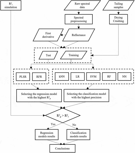
In general, the modeling workflow starts by constructing two regression models: partial least squares regression (PLSR) and random forest regression (RFR) followed selecting the best model by the highest R² value. Subsequently, the R² of the chosen model is compared to the predefined threshold (R²_t) to determine if it is greater or lower than that value. If the value is greater than the threshold, we obtain the outcome of a regression-based model and proceed to the conclusion stage; if the value is less than the threshold, classification-based models are performed. For that purpose, five classification algorithms were chosen: k-nearest neighbor (kNN), logistic regression (LR), support vector machine (SVM), random forest (RF), and neural network (NN), where each algorithm has its own advantages and disadvantages. The study’s workflow is presented in Figure 1.

Figure 1. Workflow scheme outlining the methodological concept for each data set.

Several studies have implemented the different methods to find the best classification algorithm in the remote sensing field. For example, Adelabu et al. (2013) showed that SVM provided higher accuracy than RF for tree species classification and Thanh Noi and Kappas (2018) concluded that SVM produced the highest overall accuracy compared to RF and kNN. On the other hand, Adam et al. (2014) and Ghosh and Joshi (2014) showed that SVM and RF provide similar classification results while Sluiter and Pebesma (2010) found that NN outperformed these two methods.

With that saying, the proposed work process is not only intended to predict the chemical-physical tailing parameters but also seeks to answer three important questions: (1) What is the proper way to compare R² provided by different measuring scales (laboratory, field, and image)? (2) Should regression models be seen as suppliers of a “final product”, or should they be part of a holistic prediction system? (3) How to set a threshold from which regression models (first part of the prediction system) are rejected and classification models (second part of the prediction system) are accepted.

Materials

Study area and field work

The study area is a tailing pond located 8 km northeast to the city of Erdenet, Mongolia (49°5ʹ50”N and 104°6ʹ30”E) in an elevation of approximately 1290 m above sea level. From its northwestern side to its southeastern side, the area stretches for 6.5 km and covers an area of about 20 km². The tailing area contains the material remnants that remained after the process of separating the valuable fraction (copper and molybdenum) from the ore. The ore is originated from the open-pit mine of the Erdenet porphyry copper-molybdenum deposit located 6 km east of Erdenet, Mongolia. This region is part of the Selenge intrusive complex consisting predominantly of late Permian granodiorite (Malyutin et al., 2007), andesite, diorite, granite and breccias (Gerel et al., 2005). According to the Erdenet mining company (www.erdenetmc.mn), the ore body consists of minerals including chalcosine (Cu₂S), chalcopyrite (CuFeS₂), turquoise, bornite (Cu₅FeS₄), brochantite (Cu₄SO₄(OH)₆), azurite (Cu₃(CO₃)₂(OH)₂), molybdenite (MoS₂), delafossite (CuFeO₂), tenorite (CuO), sericite. For this study, we conducted two field campaigns which took place on 2nd of July 2019 (first field work) and 30th of August 2019 (second field work) in which a total of 169 tailing samples were collected for analysis (60 samples in July and 109 in August). The sampling was performed in several cross sections along the tailing surface as well as from the subsurface to take both the spatial and vertical variabilities into account. Therefore, although most of the samples (101 samples) were collected from the surface level for the purpose of the imaging data validation, 68 samples were collected from the subsurface in 3 cm (1 sample), 5 cm (3 samples), 10 cm (1 sample), 20 cm (61 samples), 30 cm (1 sample) and 40 cm (1 sample). These also include five samples collected in a single tailing profile from the surface up to a depth of 40 cm. Due to the unattainability of some areas of the tailing pond due to high moisture content or open water bodies, the locations of the sampling points were determined in-situ mostly in areas that are as dry, accessible, and homogeneous as possible. The sampling points were geolocated with a Trimble R10 GNSS with 5 cm accuracy. Figure 2a–e presents maps of the study areas and the locations of the sampling points.

Figure 2. The study area and the sampling locations. (a) A map of Mongolia and the location of Erdenet. (b) The tailing area on a digital elevation model (Farr et al., 2007). (c) Worldview-3 RGB image as a base-map of the tailing acquired on 11.06.2019, including the sampling locations. (d) Sampling locations in the north-west side. (e) Sampling locations in the south-east side.

Spectral data acquisition

Field and laboratory reflectance measurements

The acquisition of the spectral information both in the field and laboratory has been conducted using a portable Spectral Evolution SR-3500 spectrometer equipped with an open fiber of 25° field of view. A Zenith Lite™ panel served as a white reference for calibrating the instrument to absolute reflectance values. The spectrometer has a spectral range of 350–2500 nm which covers the VIS-NIR-SWIR and it has spectral resolutions of 2.8, 8, and 6 nm at 700, 1500, and 2100 nm, respectively (Spectral Evolution). Each sampling location in the field as well as each sample in the laboratory, was measured three times. For the field measurements, the open fiber was placed approximately 1 m above the surface resulting in a measurement diameter of ca. 40 cm. For laboratory measurements, a lamp equipped with a 50 W bulb served as a light source and the open fiber was placed 15 cm above the sample resulting in a measurement diameter of ca. 7 cm.

Hyperspectral airborne imaging

The hyperspectral data collection was conducted with two HySpex imaging spectrometers (http://www.hyspex.no): the VNIR1600 covering the spectral ranges of 400–1000 nm in 160 bands and the SWIR320me covering the spectral range of 1000–2500 nm in 256 bands. Both instruments were installed on a Cessna 208B. The flight altitude was 1500 m which resulted in a nominal spatial resolution of 0.5 m and 1 m for the VNIR and SWIR imagery, respectively. In this study, we analyzed four flight lines covering the north-eastern part of the tailing.

The datasets

Since the data was collected at three levels of acquisition (laboratory, field and airborne), the analysis is performed on each dataset, separately. The laboratory dataset contains 169 spectra of dried and homogenized tailing samples that were taken from the surface as well as several subsurface samples. The field dataset contains 103 spectra acquired from the undisturbed tailing surfaces at the same exact locations from which the laboratory samples were collected. The airborne dataset contains 65 spectra extracted from the HySpex imagery coinciding with the positions of the field measurements.

Geochemical, mineralogical, and textural analysis

During the field work, Cu, Mo, and Fe contents were measured using a Niton XL3t XRF portable X-Ray fluorescence analyzer (Thermo Fisher Scientific) on the undisturbed surface samples. In-situ moisture content measurements were conducted with the ML2x ThetaProbe sensor (Delta-T devices Ltd). The geochemical and mineralogical composition of the collected samples were determined in the Central Geological Laboratory (CGL) in Ulan Baatar, Mongolia. Cu and Mo were also measured in laboratory using ICP-OES technique. For quality control purposes, the laboratory used certified reference materials (CRM) and the mean accuracy (% error) for Cu and Mo was −1.16% and 1.14%, respectively. The quality control for the XRF measurements, was performed by calculating the precision of the measurements of a specific target (mean ± standard deviation) which resulted in 0.08 ± 0.008% for Cu (field), and 0.01 ± 0.00% for Mo (field). The mineralogical analysis was performed using a semi-quantitative approach with stereoscopic microscopes (Nikon SMZ-1B, SMZ800N, Olympus SZX16) based on the principles of visual determination of minerals based on physical properties and micro-chemical methods, and quantification of the content. The sample processing is based on the specific gravity and magnetic properties of the mineral.

Particle size analysis was performed using a HELOS/KR laser diffraction (LD) analyzer with a QUIXEL dispersing system (Sympatec, GmbH) at the Institute of Geosciences and Geography of the Martin Luther University Halle-Wittenberg, Germany. The texture was classified as clay (<2 μm), silt (2–63 μm), very fine sand (63–125 μm), fine sand (125–200 μm), medium sand (200–630 μm), coarse sand (630–1250 μm), very coarse sand (1250–2000 μm), and the sum of all sand segments (63–2000 μm) according to the world reference base (WRB) soil classification system. Figure 3 and Table 1 present the results of the chemical and mineralogical analysis.

Figure 3. Violin plots of the geochemical data. These includes elements, minerals, oxides, particle size and water contents.

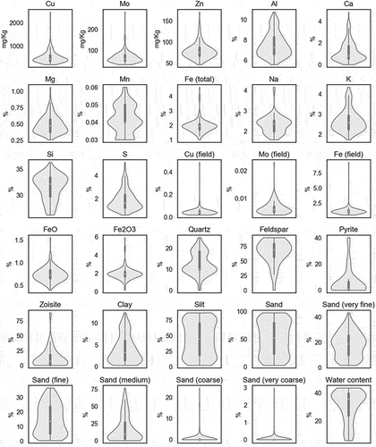
Table 1. The total number of samples (No.) and the mean and standard deviation (sd) of the geochemical parameters used in laboratory, field, and image datasets.

Parameter	Unit	Method	Laboratory			Field			Image (airborne)
			No.	mean	sd	No	mean	sd	No	mean	sd
Cu	mg kg^−1	ICP-OES	169	515.4	268.2	103	496.8	278.4	68	465.3	165.2
Mo	mg kg^−1	ICP-OES	169	66.4	27.8	103	67.5	30.7	68	62.9	24.1
Zn	mg kg^−1	ICP-OES	169	78.6	18.8	103	79.7	19.9	68	79.8	17.2
Al	%	ICP-OES	169	7.52	1.17	103	7.41	1.17	68	7.72	1.13
Ca	%	ICP-OES	169	1.20	0.92	103	1.59	0.98	68	1.89	1.07
Mg	%	ICP-OES	169	0.49	0.13	103	0.49	0.14	68	0.50	0.14
Mn	%	ICP-OES	86	0.04	0.01	57	0.04	0.01	57	0.04	0.01
Fe (total)	%	ICP-OES	169	1.94	0.46	103	1.97	0.51	68	1.96	0.46
Na	%	XRF-44	86	2.32	0.42	57	2.27	0.47	57	2.25	0.48
K	%	XRF-44	86	2.68	0.54	57	2.59	0.55	57	2.61	0.56
Si	%	XRF-44	169	31.49	2.43	103	30.86	2.62	68	30.25	2.66
S	%	Grav-13	169	1.88	0.88	103	2.25	0.93	68	2.47	0.95
Cu (field)	%	XRF	120	0.05	0.04	97	0.04	0.05	64	0.04	0.02
Mo (field)	%	XRF	112	0.007	0.002	87	0.006	0.003	55	0.006	0.002
Fe (field)	%	XRF	127	1.15	0.79	103	1.19	0.86	68	1.11	0.32
FeO	%	Titr-07	169	0.73	0.15	103	0.75	0.16	68	0.79	0.17
Fe2O3	%	Calculated	169	1.97	0.66	103	1.99	0.70	68	1.94	0.60
Quartz	%	XRD	34	12.59	5.17	36	12.05	6.03	32	12.07	6.36
Feldspar	%	XRD	34	65.39	20.38	36	61.29	24.78	32	58.82	25.47
Pyrite	%	XRD	34	5.99	9.96	36	5.49	9.80	32	5.38	9.98
Zoisite	%	XRD	34	12.16	17.32	36	17.14	26.26	32	19.15	27.61
Clay	%	LD	169	4.04	3.09	101	4.14	3.18	67	4.42	3.32
Silt	%	LD	169	44.88	27.13	101	41.41	26.69	67	49.09	27.09
Sand	%	LD	169	51.09	30.01	101	54.45	29.73	67	46.49	30.18
Sand (very fine)	%	LD	169	18.17	9.80	101	17.14	8.98	67	17.68	10.64
Sand (fine)	%	LD	169	14.94	10.20	101	27.63	19.32	67	13.49	10.64
Sand (medium)	%	LD	169	17.26	18.73	101	8.12	9.97	67	13.73	14.66
Sand (coarse)	%	LD	169	0.66	2.80	101	1.24	3.59	67	1.45	4.40
Sand (very coarse)	%	LD	169	0.05	0.32	101	0.33	1.39	67	0.13	0.51
Water content	%	Probe				68	30.54	11.20	68	30.77	11.23

Table 1. The total number of samples (No.) and the mean and standard deviation (sd) of the geochemical parameters used in laboratory, field, and image datasets.

Methods

Data preprocessing

Prior to the spectral analysis, the datasets have undergone several preprocessing steps using the Exelis ENVI/IDL 5.3 programming and image analysis environment and Python 3.9 (Van Rossum & Drake, 2009). For the laboratory and field spectra, we averaged the three spectral measurements acquired for each sample, noisy bands removal, calibration to absolute reflectance values using a white reference, and applying the Savitzky-Golay (S-G) smoothing filter (Savitzky & Golay, 1964) with a second polynomial order and a filter window of 11 bands.

The airborne hyperspectral data was corrected radiometrically using an internal software provided by NEO. The correction is performed on dark values, gain and offset of for each individual pixel, bad and blinking pixels and lens effects based on a laboratory calibration, and is described in more detailed in Lenhard et al. (2014). The geometric correction of the dataset was based on the GNSS/INS data using GNSS base-station which were positioned in Erdenet, providing an absolute accuracy of 2 cm in the XYZ space. The angle accuracy for the for the omega, phi and kappa was increased using a Kalman filter based on the GNSS trajectory with an accuracy higher than 0.003 gon. The rectification of the HySpex data was realized by timestamping every 32nd scanline with approximation of the lines between based on the higher recorded GNSS/INS trajectory. The resulting file was then integrated into Parge software (Schlaepfer et al., 1998). The atmospheric correction was conducted using the ATCOR software (Richter & Schläpfer, 2011) which is based on a flexible water vapor estimation and a flat model used for correction of solar irradiance and the atmospheric effects. After these three fundamental corrections have been applied, we performed image mosaicking and combining the VNIR and SWIR images followed by a correction of sensors shifts, removal of noisy bands affected by atmospheric water vapor absorptions and overlapping bands, as well as S-G spectral smoothing using the second polynomial order and a filter window of 11 bands.

The spectral analysis has been conducted using either the reflectance or the first derivative spectra. For outlier detection, the z-score method has been used which removes any sample that is greater than three standard deviations (sd) from the mean (Eq. 1)(1) $\mathrm{Z}\mathrm{s}\mathrm{c}\mathrm{o}\mathrm{r}\mathrm{e}=\frac{\mathrm{x}-\mathrm{m}\mathrm{e}\mathrm{a}\mathrm{n}}{\mathrm{s}\mathrm{d}}$(1) :

(1) $\mathrm{Z}\mathrm{s}\mathrm{c}\mathrm{o}\mathrm{r}\mathrm{e}=\frac{\mathrm{x}-\mathrm{m}\mathrm{e}\mathrm{a}\mathrm{n}}{\mathrm{s}\mathrm{d}}$(1)

Statistical analysis

Statistical analysis for the purpose of calibration and validation of the regression and classification models has been conducted using the scikit-learn python module (Pedregosa et al., 2011).

Regression models

Two types of regression models were used for the analysis: partial least squares regression (PLSR) and random forest regression (RFR). The samples in each dataset were divided into training and test samples in an 80:20 ratio with the same value given to the random state property, which uses the sample division in both PLSR and RFR. PLSR is a robust linear prediction method that has been successfully used in spectroscopy and remote sensing for predicting various geochemical, mineralogical, and textural parameters. Additionally, it enables modeling when the multicollinearity of independent variable sets exists or the sample size is smaller than the number of independent variables (Sjöström et al., 1983). The RFR was proposed by Breiman (2001) and is a powerful and an accurate prediction model technique based on classification and regression trees, which includes features with non-linear relationship.

Classification models

For classification purposes, the following algorithms were used: kNN, LR, SVM, RF, and NN. kNN is the most widely used non-parametric classification method which uses the Euclidian distance between the points while assuming that the data is homogeneous (K. Huang et al., 2015; Song et al., 2016). LR is a widely used statistical direct probability model which estimates the probability for a given feature (x) and the label (y) directly from the training data by minimizing the error (Ng & Jordan, 2002; Tsangaratos & Ilia, 2016). SVM which was proposed by Boser et al. (1992) is a supervised classification method that appears to be advantageous in the presence of heterogenous classes for which only few training samples are available (Melgani & Bruzzone, 2004). The SVM employs optimization algorithms to locate the optimal boundaries between classes by minimizing the confusion between them (C. Huang et al., 2002) and it plays a huge role in image processing (Lv & Wang, 2020). RF is a tree-based classifier which grows an ensemble of decision trees and allowing them to vote for the most popular class. RF produced a significant increase in classification accuracy for land cover classification (Breiman, 2001; Pal, 2005). RF features a relatively high accuracy and a rapid processing time (Gogineni & Chaturvedi, 2019). NN is one of the most widely used artificial intelligence classification method and it is used in image classification and is characterized by simulating the processing mechanism by human neurons. However, due to the high level of complexity, it has a slower operation speed compared to other classification methods and it requires a large amount of training data (Lv & Wang, 2020).

Models’ evaluation

The performance of the regression models was evaluated using the coefficient of determination (R²) which is the ratio of the explained variation to the total variation, and the root mean squared error (RMSE) which is the standard deviation of the residuals. These are calculated using Eq. (2(2) ${\text{R}}^2=\frac{{\displaystyle {\sum }_{\text{i}=1}^{\text{n}}{\left({\widehat{y}}_{\text{i}}-\overline{y}\right)}^2}}{{\displaystyle {\sum }_{\text{i}=1}^{\text{n}}{\left({\text{y}}_{\text{i}}-\overline{y}\right)}^2}}$(2) –3(3) $\text{RMSE}=\sqrt{\frac{{\displaystyle {\sum }_{\text{i}=1}^{\text{n}}{\left({\widehat{y}}_{\text{i}}-{\text{y}}_{\text{i}}\right)}^2}}{\text{n}}}$(3) ):

(2) ${\text{R}}^2=\frac{{\displaystyle {\sum }_{\text{i}=1}^{\text{n}}{\left({\widehat{y}}_{\text{i}}-\overline{y}\right)}^2}}{{\displaystyle {\sum }_{\text{i}=1}^{\text{n}}{\left({\text{y}}_{\text{i}}-\overline{y}\right)}^2}}$(2)

(3) $\text{RMSE}=\sqrt{\frac{{\displaystyle {\sum }_{\text{i}=1}^{\text{n}}{\left({\widehat{y}}_{\text{i}}-{\text{y}}_{\text{i}}\right)}^2}}{\text{n}}}$(3)

Where ${\hat{y}}_i$ and $y_i$ are the predicted and the true values of the $i$-th sample, respectively, $n$ is the number of samples and $\bar{y}$ is the mean (Esbensen et al., 2002).

The performance of the classification models was evaluated by their precision which can be calculated using Eq. (4)(4) $\mathrm{P}\mathrm{r}\mathrm{e}\mathrm{c}\mathrm{i}\mathrm{s}\mathrm{i}\mathrm{o}\mathrm{n}=\frac{\mathrm{t}\mathrm{p}}{\mathrm{t}\mathrm{p}+\mathrm{f}\mathrm{p}}$(4) :

(4) $\mathrm{P}\mathrm{r}\mathrm{e}\mathrm{c}\mathrm{i}\mathrm{s}\mathrm{i}\mathrm{o}\mathrm{n}=\frac{\mathrm{t}\mathrm{p}}{\mathrm{t}\mathrm{p}+\mathrm{f}\mathrm{p}}$(4)

Where $tp$ is the number of true positive cases and $fp$ is the number of false positive cases (Davis & Goadrich, 2006).

Due to the complexity of the workflow, the results were evaluated in four key points that would allow us to choose the most suitable method for further analysis. The evaluation was performed in the following crossroads which compare between:

1. Preprocessing method (Ref, fDer).

2. Regression-based method (PLSR or RFR).

3. Classification-based methods (kNN, LR, SVM, RF, NN)

All of these are state of the art and robust methods which are feasible in the fields of spectroscopy and remote sensing and applicable in the mining industry. It should be clarified that due to the relatively small sample size in the imaging datasets, the models were evaluated using the R² of the cross-validation instead of using the R² (prediction).

Procedure for estimating the R²_t

The quality and accuracy of the field spectra and imaging data is lower than the spectra obtained in the laboratory due to variations in surface humidity, the presence of atmospheric water vapor and inconsistent solar radiation, and the quality of the atmospheric correction accompanied with differences in the spatial resolution. These effects cause an uncertainty which is reflected in the predictive capabilities of the regression models. Therefore, apart from using R² which estimates the model’s consistency, we established an R² threshold (R²_t) below which the regression-based model is rejected, and classification-based models are to be used. The R²_t does not specify whether the regression model is successful or not, but whether a classification-based model is preferred.

Since the degree of error and thus, the uncertainty in laboratory measurements is very small, the threshold should be set high and would be dependent on the value of R² providing a classification with a 100% accuracy. And since the error in the field and image data is high, the threshold values are set lower than in laboratory. For that purpose, we follow the findings of Jiménez et al. (2018) and Gomez et al. (2008) and set an error of 10% between laboratory and field and 20% between laboratory and airborne results.

Subsequently, we build a confusion matrix on top of a Cartesian axis structure, containing a certain number of samples. In the first stage 50% of the samples were randomly given x and y values between 50 and 100 (true high) and 50% of the samples were randomly given x and y values between 0 and 50 (true low). Hence, 100% of the samples were classified as true.

In the second stage, the samples were divided 90% true and 10% false, and in the third stage 80% true and 20% false. We repeated this procedure for each stage 30 times, while calculating the R² result for each run followed by calculating its average value.

The calculated R²_t is then subtracted from the R² of prediction (R²_p). If the outcome is zero or positive (Eq. 5(5) ${\mathrm{R}}_{\mathrm{p}}^2\ge {\mathrm{R}}_{\mathrm{t}}^2\to \mathrm{R}\mathrm{e}\mathrm{g}\mathrm{r}\mathrm{e}\mathrm{s}\mathrm{s}\mathrm{i}\mathrm{o}\mathrm{n}\mathrm{m}\mathrm{o}\mathrm{d}\mathrm{e}\mathrm{l}\mathrm{s}$(5) ), we accept the regression model and proceed to the conclusions. However, if the outcome is negative (Eq. 6(6) ${\mathrm{R}}_{\mathrm{p}}^2<{\mathrm{R}}_{\mathrm{t}}^2\to \mathrm{C}\mathrm{l}\mathrm{a}\mathrm{s}\mathrm{s}\mathrm{i}\mathrm{f}\mathrm{i}\mathrm{c}\mathrm{a}\mathrm{t}\mathrm{i}\mathrm{o}\mathrm{n}\mathrm{m}\mathrm{o}\mathrm{d}\mathrm{e}\mathrm{l}\mathrm{s}$(6) ), we conclude that the prediction based on regression models is unsatisfactory and move on to examining the performance of the classification-based models.

(5) ${\mathrm{R}}_{\mathrm{p}}^2\ge {\mathrm{R}}_{\mathrm{t}}^2\to \mathrm{R}\mathrm{e}\mathrm{g}\mathrm{r}\mathrm{e}\mathrm{s}\mathrm{s}\mathrm{i}\mathrm{o}\mathrm{n}\mathrm{m}\mathrm{o}\mathrm{d}\mathrm{e}\mathrm{l}\mathrm{s}$(5)

(6) ${\mathrm{R}}_{\mathrm{p}}^2<{\mathrm{R}}_{\mathrm{t}}^2\to \mathrm{C}\mathrm{l}\mathrm{a}\mathrm{s}\mathrm{s}\mathrm{i}\mathrm{f}\mathrm{i}\mathrm{c}\mathrm{a}\mathrm{t}\mathrm{i}\mathrm{o}\mathrm{n}\mathrm{m}\mathrm{o}\mathrm{d}\mathrm{e}\mathrm{l}\mathrm{s}$(6)

Due to the uncertainty factor, comparing models built from laboratory, field, and image data based on their R² values might be problematic. Therefore, each model should be compared to the performance potential of the same acquisition space where the total uncertainty estimate is found. This means that in different acquisition levels and their associated inaccuracies should be considered when assessing the R² values.

Results

Geochemistry’s correlation matrix

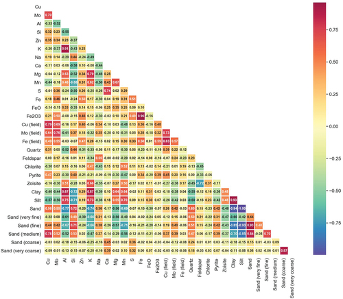
Because of the large number of variables, a correlation matrix displaying the correlation coefficients between the geochemical parameters in the database is helpful. This will allow the prediction of one parameter using another without having to create a new statistical model. Example of these correlations can be seen in Figure 4, where high correlations were found between Cu and Mo (R = 0.7), Al and K (R = 0.91), clay with both Al and K (R = 0.87), Quartz shows the highest positive correlation with Si (R = 0.44). In addition, feldspar display its highest correlation with Na (R = 0.55) which may indicate that the relative share of the mineral Albite (NaAlSi₃O₈) is the highest compared to other feldspar endmembers such as potassium feldspar (K-spar) and calcium-rich feldspar (anorthite). (Khajehzadeh et al., 2017) reported that the correlation coefficient between quartz and Fe to be remarkably high (R = −0.96) using only a set of 14 samples. However, as shown in Figure 4 a lower correlation was obtained (R = −0.23) between these two parameters in our study but its negative direction is still maintained which can be explained by the difference in the number of samples used in the current study.

Figure 4. Correlation coefficients between the geochemical contents.

Geochemical prediction workflow

Estimating the R²_t

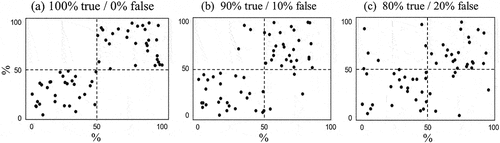
The simulation included three configurations which are presented in Figure 5. In the first configuration the threshold was calculated using 34 samples, 22 samples in the second, and 14 samples in the third, which simulate the number of test samples used in the regression-based models in the laboratory, field, and imaging datasets, respectively. The increase of uncertainty is expressed by the decrease of the percentage of the samples which are classified as “true high” and “true low”.

Figure 5. An example of the simulation for predicting the threshold of R2. (a) uses samples that are distributed randomly where 100% of the samples were classified as true (positive or negative), (b) shows 90% true and 10% false, and in (c) 80% were classified as true and 20% as false. The X-axis and Y-axis both have arbitrary values between 0 to 100% to facilitate the presenting of simulation results.

After performing the simulation, we could quantify the value of R²_t for each dataset according to its estimated uncertainty level which are shown in Table 2. It is worth noting that the sample size had no impact on the result, implying that the change in R²_t is entirely due to the preliminary classification. The simulated laboratory dataset provided the highest value with an R²_t = 0.58, followed by field dataset with an R²_t = 0.4, and for the airborne image dataset with an R²_t = 0.31. Following this step, we can now build regression models and assess their performance by comparing their R²_p to the R²_t.

Table 2. The number of samples and the percent of samples that are classified as true (high and low) used for simulating the R²_t.

Simulated Dataset	No. of Samples	% True	R^2t
Laboratory	34	100	0.58
Field	22	90	0.40
Image (airborne)	14	80	0.31

Table 2. The number of samples and the percent of samples that are classified as true (high and low) used for simulating the R²_t.

Modeling of laboratory data

Regression models were calculated for 26 geochemical, mineralogical, and textural parameters, of which 13 parameters were predicted using regression models (PLS or RFR) where R²_p > R²_t, while the remaining 13 parameters were predicted using classification models. The highest R² values were obtained for particle sizes clay, silt, and sand with R² = 0.92, 0.95, 0.94 and RMSEP = 0.92, 6.51, 7.56, respectively. For the subdivision of sand i.e. sand (very fine), sand (fine), and sand (medium), the R² was 0.71, 0.86, 0.93 and the RMSEP = 5.39, 3.84, and 5.64, respectively. For Al, Cu, Si, S, K, Ca, and Mg R² were 0.87, 0.86, 0.85, 0.77, 0.73, 0.67, 0.61 and RMSEP = 0.42, 76.75, 1.05, 0.43, 0.32, 0.5, and 0.08, respectively. Water content was neglected from the modeling because the samples were measured after drying under laboratory conditions.

All other parameters were analyzed using the classification-based models with an average precision of 0.74 where the lowest precision of 0.58 was obtained for Zn and the highest precision of 1 for zoisite. Even though some minerals such as quartz, feldspar and pyrite do not exhibit any spectral features in the VNIR-SWIR and regression-based models could not perform valuable prediction, satisfactory results were obtained with the classification-based models with precisions of 0.64, 0.79, and 0.85, respectively.

Modeling of field data

The model performance based on field data, showed that out of a total of 27 geochemical parameters, only 12 parameters were predicted using the regression-based models. Due to the high variability of the water content within the homogeneous tailing area, it provided the highest value with R² = 0.83 and RMSEP = 4.51. The performance of the particle size models was still good, with R² = 0.63, 0.55, 0.52, 0.42, 0.41 and RMSEP = 10.91, 5.14, 2.18, 19.28, and 21.75 for sand (fine), sand (medium), clay, silt, and sand, respectively. For Si, S, Ca, Cu, and K, the R² ranges between 0.45 and 0.56 and the RMSEP between 0.41 and 1.84 (for more detailed information see, Table 3). An interesting parameter with a R² > R²_t was the Cu (field) content with R² = 0.42 and RMSEP = 0.02. This result shows that although the field measurements have been conducted under varying moisture/wetness conditions, the variability of the Cu content was high enough for providing a satisfactory regression-based model result. The results for classification-based models showed an average precision of 0.73, ranging between 0.57 for Zoisite and 0.91 for both Na and Fe (field).

Table 3. Summary of selected regression-based and classification-based models according to the proposed workflow.

	Laboratory (R^2t = 0.58)				Field (R^2t = 0.4)				Image (R^2t = 0.31)
Parameter	Regression	R^2p	Classification	Precision	Regression	R^2p	Classification	Precision	Regression	R^2CV	Classification	Precision
Cu	RF	0.86	NN	0.82	RF	0.47	NN	0.76	PLS	0.42	LR/SVM	0.57
Mo											kNN/RF	0.64
Al	PLS	0.87					LR	0.76			LR	0.79
Si	PLS	0.85			RF	0.56
Zn			kNN/SVM	0.58			LR	0.81			LR	0.64
K	PLS	0.73			PLS	0.45					kNN/NN	0.5
Na			kNN/RF	0.82			LR	0.91	PLS	0.41
Ca	RF	0.67			RF	0.49			PLS	0.33
Mg	PLS	0.61					kNN/LR	0.67			kNN/LR	0.71
Mn	PLS	0.66					kNn	0.67			LR	0.67
S	PLS	0.77			PLS	0.56					kNN/SVM	0.64
Fe			RF	0.73			kNN/SVM	0.7			LR	0.86
FeO			LG/SVM	0.74			LR	0.71			LR/SVM	0.64
Fe2O3			RF	0.67			LR/NN	0.7			SVM	0.64
Cu (field)			kNN/SVM/RF	0.67	PLS	0.42					SVM/RF	0.85
Mo (field)			LR/SVM/NN	0.61			LR/SVM	0.72			SVM/RF	0.82
Fe (field)			RF	0.69			NN	0.91			SVM/RF	0.71
Quartz			LR/RF/NN	0.64			NN	0.63			kNN	0.71
Feldspar			NN	0.79			RF	0.75			LR/RF	0.71
Chlorite
Pyrite			RF/NN	0.85			SVM	0.71			LR/SVM/RF	0.83
Zoisite			SVM	1			kNN	0.57	PLS	0.41
Clay	PLS	0.92			PLS	0.52			PLS	0.36
Silt	RF	0.95			PLS	0.42			PLS	0.39
Sand	RF	0.94			PLS	0.41			PLS	0.39
Sand very fine	PLS	0.71					LR/RF	0.67			LR	0.71
Sand fine	RF	0.86			RF	0.63			PLS	0.33
Sand medium	PLS	0.93			RF	0.55			PLS	0.33
Sand coarse
Sand very
Water content					RF	0.83					LR	0.79

Modeling of image data

Acquiring a hyperspectral image over a surface with high water content combined with atmospheric corrections and further preprocessing, may adversely affect the spectral data. As a result, there have been many doubts about the ability to develop reliable models for predicting geochemical properties for the tailing area in this case study. Despite this, out of a total of 27 parameters, 9 were predicted using regression-based models. However, due to the small sample size in the image data, we used the R² and RMSE of the cross-validation (RMSECV). The highest correlation was observed for Si with R² = 0.42 and RMSECV = 2.05. For Na, Ca and zoisite the R² = 0.41, 0.33 and 0.41, and RMSECV = 0.32, 0.8 and 19.35, respectively. In addition, the grain size models also provided satisfactory results with R² between 0.33 and 0.36 and RMSECV between 2.63 and 23.81 for clay, silt, sand, sand (fine), and sand (medium). A summary of the results given by the regression- and classification-based approaches is shown in Table 3.

Table 3. Summary of selected regression-based and classification-based models according to the proposed workflow.

Discussion

The performance of regression-based models

The results indicate that the regression models accurately predicted grain size and 8 of the 12 elements studied. Surprisingly, the regression models were unable to predict iron oxides (FeO and Fe₂O₃), which are known to exhibit spectral features in the VNIR region (400–2500 nm; Pieters & Englert, 1993; Scheinost et al., 1998; Y.Z. Wu et al., 2005). However, that can be explained by the low content and low variability of FeO (0.39–1.18%) and Fe₂O₃ (0.15–3.3%) which resulted in a R² of 0.23 and 0.16 using the laboratory dataset. These results, along with the lower performance using the field and image data, were not sufficient for regression models (R²_p < R²_t); therefore, we utilized a classification-based approach for these two oxides.

VIS-NIR diffuse reflectance spectroscopy for predicting elemental concentrations was used by (Koch et al., 2017) who reported R² = 0.83, 0.67, 0.86, 0.7, 0.81, 0.64, 0.73 for Al, Cu, Si, S, K, Ca, and Mg, respectively. Their results correspond to our current study, except for the Cu content, for which the models were less good than in our study, conceivably due to the low concentration and low variability of Cu in their data. Furthermore, they reported an R² = 0.86 for Fe content which was much higher than the R² = 0.48 obtained in this study. This may be because the Fe content in their samples was between 18,625.16 and 163,863.4 mg kg⁻¹ (equivalent to 1.86% and 16.36%) compared to 1.0–2.87% in the current study. Pyo et al. (2020) also estimated the Cu content in tailing samples with the use of RFR, however despite the high variability (9.8–19,748 ppm which is equivalent to mg kg⁻¹), they achieved relatively low R² = 0.67, in comparison to the current study.

Other comparisons can be made with the field of soil science and the effect of concentration and variability of the model performance. Using PLSR, Wu et al. (2011) achieved R² = 0.55 and RMSEP = 6.49 for Cu despite the low elemental concentration. In contrast, Camargo et al. (2015) observed R² = 0.4 and 0.8 for samples with contents between 0.69–5.57% and 1.67–9.94% for FeO and Fe₂O₃, respectively. The better predictions for iron oxides are most likely due to higher contents and higher variability compared to this study.

The above results correspond to other studies that show a decrease in model performance between laboratory, field, and image datasets (see, Figure 6) due to the influence of sample size (Ng et al., 2020), surface condition (Udelhoven et al., 2003), spectral resolution and SNR (Wu et al., 2011), spatial resolution (Dkhala et al., 2020) or atmospheric conditions (Dkhala et al., 2020). It is worth noting that the drop in performance is only visible in regression models, not classification models.

Figure 6. The overall performance of regression- and classification-based models using laboratory, field, and image datasets.

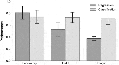
The performance of classification-based models

Unlike the regression models, the average performance of the classification-based models did not exhibit any decrease between laboratory, field, and image models. This was due to the threshold that was given for accepting the regression models. However, this may indicate that classification models even though being less precise than regression models by nature, are more stable and consistent in predicting the geochemistry. Furthermore, under uncontrolled environmental conditions in general, and high-water content in particular, classification models may be the best option for the spatial prediction of mineralogy and chemical tailing parameters.

Factors affecting the performance of the models

The model’s performance indicates that the difference between the measurement conditions is affected mainly by the number of samples, water content, surface roughness, and the preprocessing algorithms which are summarized in Table 4. In the transition between laboratory, field and image datasets, sample size was decreased while water content (between laboratory and field/image), surface roughness, and preprocessing were increased. Consequently, the ability of regression models to perform accurate predictions has diminished. To address this issue, at least partially, it is recommended to increase the sample size and target the field sampling and measurements in as flat and dry areas as possible. Also, for better mineralogical assessment, to conduct additional measurements in the MWIR-LWIR due to the presence of spectral features in these regions.

Table 4. The relative effect of the influencing factor on the performance of the models in this study.

	Laboratory	Field	Image
Sample size*	+	++	+++
Data variability*	+	+	+
Analyte concentration*	+	+	+
Water content	‒	+++	+++
Surface roughness	‒	+	++
Spectral features*	+	+	+
Data pre-processing	+	++	+++

Note: Use the following legend

* = variable dependent

(‒) = no influence

(+) = minor influence

(++) = intermediate influence

(+++) = major influence

Table 4. The relative effect of the influencing factor on the performance of the models in this study.

Limitations

There are several limitations to the proposed method that should be highlighted even in cases where optimal conditions exist. First, previous studies have shown that the estimated uncertainty between laboratory, field, and airborne data is not an exact value but a range of values that depends also on the property in question. Whereas in this study, we provide a precise threshold for each mean of measure. Although this determination is necessary for the workflow, it may neglect the precision of regression models even when R²_p is only slightly below R²_t. Thus, when a precise estimation is required, our advice is to lower the threshold of R²_t before changing to classification models. Second, in classification models, the differentiation between high and low is determined by the median value of each parameter which may change drastically as more samples are added. Therefore, to avoid that, the mean value can be used as well. Third, R² is the only value that is used in the workflow and its value can be due to over- or under-estimation. Therefore, for a more precise estimation, it is advised to add RMSE to be implemented in the workflow.

Conclusion

This study demonstrates the use of a novel method for selecting the most suitable and applicable model type (regression- or classification-based) to be used for predicting and characterizing geochemical, mineralogical, and textural parameters using laboratory, field, and image datasets. The proposed approach is based on the fact that with the transition between laboratory data, field and image, any addition of uncertainty to the spectral information caused as a result of equipment performance, methodology of measurement, sampling strategy, surface properties, and environmental conditions (Jiménez et al., 2018), will result in a decrease in model performance. To this end, we have developed a method that reduces the threshold for accepting the regression model by estimating an R² threshold (R²_t) for each level of measurement (laboratory, field, image) and comparing it to the R² obtained by the regression model. Consequently, regression models that achieved R²_p ≥ R²_t, were considered to have acceptable performance, while we considered models with R²_p < R²_t to not fulfill the necessary performance requirements. To compensate for the lack of precision, classification-based models were used afterwards to achieve a prediction result where the predicted value is either above or below the median value of the target parameter. Results show that the acceptable R²_t was reduced from 0.58 for laboratory to 0.40 for field data and then to 0.31 for the hyperspectral airborne data. As indicated previously, these values are determined from the uncertainty associated with each measurement mean. We anticipate that this method is not limited to tailing samples but can be applied on other fields of research such as pedology or agriculture.

To strengthen these conclusions and exploit the suggested guidelines, this study can be expanded to incorporate additional tailing samples, higher content and variability and include other spectral ranges such as the medium-wave and long-wave infrared (MWIR-LWIR) and the light detection and ranging (LiDAR) sensors. We anticipate that by doing so, it will be feasible to predict additional parameters such as quartz and feldspar using regression models and to improve the prediction of existing parameters utilizing point-spectroscopy and airborne data, as well as space-borne data.

Authors Contributions

Yaron Ogen is the main author of this manuscript and developed the research concept and workflow, conducted the field and laboratory spectral measurements as well as all statistical analyses presented in this study. Michael Denk conducted the field spectral measurements together with Yaron Ogen. Cornelia Glaesser and Michael Denk were involved in developing the concept for this study and substantially contributed to writing the manuscript. Holger Eichstaedt was responsible for the acquisition of the hyperspectral airborne data and performed the radiometric and atmospheric corrections.

Acknowledgments

We wish to thank the Client II program of the German Federal Ministry of Education and Research (BMBF) for funding the ADRIANA project (funding code: 033R213B). ADRIANA is conducted by a consortium of G.E.O.S., Martin Luther University (MLU), DIMAP and CBM supported by the Mongolian partners in Erdenet Mining Corporation (EMC), Erdenet Institute of Technology (EIT) and the German-Mongolian institute for Resource and Technology (GMIT). In addition, we would like to thank the staff members from EMC, EIT and GMIT, especially Mr. Tugsbuyan Tsedenbaljir, Mr. Undrakhtamir Alyeksandr, Mr. Tsedendamba Oyunbuyan, Mr. Tumendelger Batsuuri, Mr. Galsanjamts Otgonbaatar, Mr. Tushig Zolboo, and Ms. Munkhjargal Chimeddorj. To Rudolf Suppes (CBM) and Mr. Rene Kahnt and Mr. Ralf Loeser (G.E.O.S) for their assistance during the field work. A special gratitude to Mr. Dennis Sakretz for sample preparation and Mr. Michael von Hoff for performing the laser diffraction particle-size analysis.

Data Availability Statement

Due to the nature of this research, participants of this study did not agree for their data to be shared publicly, so supporting data is not available.

Disclosure statement

No potential conflict of interest was reported by the author(s).

Additional information

Funding

This work was supported by the Client II program of the German Federal Ministry of Education and Research (BMBF) [033R213B].

References

- Adam, E., Mutanga, O., Odindi, J., & Abdel-Rahman, E. M. (2014). Land-use/cover classification in a heterogeneous coastal landscape using RapidEye imagery: Evaluating the performance of random forest and support vector machines classifiers. International Journal of Remote Sensing, 35(10), 3440–3458.
- Adelabu, S., Mutanga, O., Adam, E. E., & Cho, M. A. (2013). Exploiting machine learning algorithms for tree species classification in a semiarid woodland using RapidEye image. Journal of Applied Remote Sensing, 7(1), 073480.
- Aubertin, M., Ricard, J.-F., & Chapuis, R. P. (1998). A predictive model for the water retention curve: Application to tailings from hard-rock mines. Canadian Geotechnical Journal, 35(1), 55–69.
- Awad, M. E., Amer, R., López-Galindo, A., El-Rahmany, M. M., García Del Moral, L. F., & Viseras, C. (2018). Hyperspectral remote sensing for mapping and detection of Egyptian kaolin quality. Applied Clay Science, 160, 249–262. https://doi.org/10.1016/j.clay.2018.02.042
- Ben‐Dor, E., Taylor, R. G., Hill, J., Demattê, J. A. M., Whiting, M. L., Chabrillat, S., & Sommer, S. (2008). Imaging Spectrometry for Soil Applications. In Advances in Agronomy (pp. 321–392). Academic Press. https://doi.org/10.1016/S0065-2113(07)00008-9
- Boser, B. E., Guyon, I. M., & Vapnik, V. N. (1992). A training algorithm for optimal margin classifiers. In Proceedings of the fifth annual workshop on computational learning theory (pp. 144–152). New York, NY, USA: Association for Computing Machinery
- Breiman, L. (2001). Random Forests. Machine Learning, 45(1), 5–32.
- Brown, G. E., Foster, A. L., & Ostergren, J. D. (1999). Mineral surfaces and bioavailability of heavy metals: A molecular-scale perspective. Proceedings of the National Academy of Sciences, 96(7), 3388–3395.
- Camargo, L. A., Marques, J., Barrón, V., Alleoni, L. R. F., Barbosa, R. S., & Pereira, G. T. (2015). Mapping of clay, iron oxide and adsorbed phosphate in Oxisols using diffuse reflectance spectroscopy. Geoderma, 251–252, 124–132. https://doi.org/10.1016/j.geoderma.2015.03.027
- Carmon, N., Thompson, D. R., Bohn, N., Susiluoto, J., Turmon, M., Brodrick, P. G., Connelly, D. S., Braverman, A., Cawse-Nicholson, K., Green, R. O., & Gunson, M. (2020). Uncertainty quantification for a global imaging spectroscopy surface composition investigation. Remote Sensing of Environment, 251, 112038. https://doi.org/10.1016/j.rse.2020.112038
- Clark, R. N. (1999). Chapter 1: spectroscopy of rocks and minerals, and principles of spectroscopy, in manual of remote sensing. In A.N. Rencz (Ed.), Remote sensing for the earth sciences (Vol. 3, pp. 3–58). John Wiley and Sons.
- Clark, R., Boardman, J., Mustard, J., Kruse, F., Ong, C., Pieters, C., & Swayze, G. (2006). Mineral mapping and applications of imaging spectroscopy. In 2006 IEEE international symposium on geoscience and remote sensing, pp. 1986–1989.
- Cudahy, T. J., Hewson, R., Huntington, J. F., Quigley, M. A., & Barry, P. S. (2001). The performance of the satellite-borne hyperion hyperspectral VNIR-SWIR imaging system for mineral mapping at Mount Fitton, South Australia. In IGARSS 2001. scanning the present and resolving the future. proceedings. IEEE 2001 International Geoscience and Remote Sensing Symposium (Cat. No. 01CH37217) (pp. 314–316). vol.1.
- Davis, J., & Goadrich, M. (2006). The relationship between precision-recall and ROC curves. In Proceedings of the 23rd international conference on machine learning (pp. 233–240). New York, NY, USA: Association for Computing Machinery
- DiFoggio, R. (2000). Guidelines for applying chemometrics to spectra: Feasibility and error propagation. Applied Spectroscopy, 54(3), 94A–113A.
- Dkhala, B., Mezned, N., Gomez, C., & Abdeljaouad, S. (2020). Hyperspectral field spectroscopy and SENTINEL-2 Multispectral data for minerals with high pollution potential content estimation and mapping. Science of the Total Environment, 740, 140160. https://doi.org/10.1016/j.scitotenv.2020.140160
- Engel, J., Gerretzen, J., Szymańska, E., Jansen, J. J., Downey, G., Blanchet, L., & Buydens, L. M. C. (2013). Breaking with trends in pre-processing? TrAC - Trends in Analytical Chemistry, 50, 96–106. https://doi.org/10.1016/j.trac.2013.04.015
- Esbensen, K. H., Guyot, D., Westad, F., & Houmoller, L. P. (2002). Multivariate data analysis. In Practice: An introduction to multivariate data analysis and experimental design. Multivariate Data Analysis.
- Farr, T. G., Rosen, P. A., Caro, E., Crippen, R., Duren, R., Hensley, S., Kobrick, M., Paller, M., Rodriguez, E., Roth, L., Seal D. (2007). The shuttle radar topography mission. Reviews of Geophysics45(2):45. https://doi.org/10.1029/2005RG000183
- Feng, J., Rogge, D., & Rivard, B. (2018). Comparison of lithological mapping results from airborne hyperspectral VNIR-SWIR, LWIR and combined data. International Journal of Applied Earth Observation and Geoinformation, 64, 340–353. https://doi.org/10.1016/j.jag.2017.03.003
- Fenstermaker, L. K., & Mlller, J. R. (1994). ldentification of fluvially redistributed mill tailings using high spectral resolution airctaft. Photogrammetric Engineering and Remote Sensing, 60(8): 989–995.
- Forina, M., Lanteri, S., & Todeschini, R. (2000). Chemometrics for sampling and analysis: theory and environmental applications. In Chemical processes in marine environments (pp. 387–404). Springer).
- Gerel, O., Dandar, S., Amar-Amgalan, S., Javkhlanbold, D., Myagamarsuren, S., Myagmarsuren, S., Munkhtsengel, B., & Soyolmaa, B. (2005). Geochemistry of granitoids and alteRed rocks of the erdenet porphyry copper-molybdenum deposit, central Mongolia. In J. Mao & F.P. Bierlein (Eds.), Mineral deposit research: meeting the global challenge (pp. 1137–1140). Springer.
- Ghosh, A., & Joshi, P. K. (2014). A comparison of selected classification algorithms for mapping bamboo patches in lower Gangetic plains using very high resolution WorldView 2 imagery. International Journal of Applied Earth Observation and Geoinformation, 26, 298–311. https://doi.org/10.1016/j.jag.2013.08.011
- Gogineni, R., & Chaturvedi, A. (2019). Hyperspectral image classification. Processing and Analysis of Hyperspectral Data, (Intechopen). doi:10.5772/intechopen.88925
- Gomez, C., Lagacherie, P., & Coulouma, G. (2008). Continuum removal versus PLSR method for clay and calcium carbonate content estimation from laboratory and airborne hyperspectral measurements. Geoderma, 148(2), 141–148.
- Gomez, C., Oltra-Carrió, R., Bacha, S., Lagacherie, P., & Briottet, X. (2015). Evaluating the sensitivity of clay content prediction to atmospheric effects and degradation of image spatial resolution using Hyperspectral VNIR/SWIR imagery. Remote Sensing of Environment, 164, 1–15. https://doi.org/10.1016/j.rse.2015.02.019
- Götze, C., Denk, M., Riedel, F., & Gläßer, C. (2017). Interlaboratory comparison of spectrometric laboratory measurements of a chlorite rock sample. PFG - Journal of Photogrammetry, Remote Sensing and Geoinformation Science, 85(5), 307–316.
- Hao, L., Zhang, Z., & Yang, X. (2019). Mine tailing extraction indexes and model using remote-sensing images in southeast Hubei Province. Environmental Earth Sciences, 78(15), 493.
- Huang, C., Davis, L. S., & Townshend, J. R. G. (2002). An assessment of support vector machines for land cover classification. International Journal of Remote Sensing, 23(4), 725–749.
- Huang, K., Li, S., Kang, X., & Fang, L. (2015). Spectral–spatial hyperspectral image classification based on KNN. Sensing and Imaging, 17(1), 1.
- Jiménez, M., de la Cámara, O. G., Moncholí, A., & Muñoz, F. (2018). Towards a complete spectral reflectance uncertainty model for Field Spectroscopy. Fifth Recent Advances in Quantitative Remote Sensing, 21.
- Khajehzadeh, N., Haavisto, O., & Koresaar, L. (2017). On-stream mineral identification of tailing slurries of an iron ore concentrator using data fusion of LIBS, reflectance spectroscopy and XRF measurement techniques. Minerals Engineering, 113, 83–94. https://doi.org/10.1016/j.mineng.2017.08.007
- King, P. L., Ramsey, M. S., & Swayze, G. A. (2004). Infrared spectroscopy in geochemistry, exploration geochemistry and remote sensing. Mineralogical Association of Canada.
- Koch, J., Chakraborty, S., Li, B., Kucera, J. M., Van Deventer, P., Daniell, A., Faul, C., Man, T., Pearson, D., Duda, B., Weindorf, C. A., & Weindorf, D. C. (2017). Proximal sensor analysis of mine tailings in South Africa: An exploratory study. Journal of Geochemical Exploration, 181, 45–57. https://doi.org/10.1016/j.gexplo.2017.06.020Get
- Lagacherie, P., Baret, F., Feret, J.-B., Madeira Netto, J., & Robbez-Masson, J. M. (2008). Estimation of soil clay and calcium carbonate using laboratory, field and airborne hyperspectral measurements. Remote Sensing of Environment, 112(3), 825–835.
- Langsdale, M. F., Wooster, M., Harrison, J. J., Koehl, M., Hecker, C., Hook, S. J., Abbott, E., Johnson, W. R., Maturilli, A., Poutier, L., Lau, I., & Brucker, F. (2021). Spectral emissivity (SE) measurement uncertainties across 2.5–14 μm derived from a round-robin study made across international laboratories. Remote Sensing, 13(1), 102.
- Lenhard, K., Baumgartner, A., & Schwarzmaier, T. (2014). Independent laboratory characterization of NEO HySpex imaging spectrometers VNIR-1600 and SWIR-320m-e. IEEE Transactions on Geoscience and Remote Sensing, 53(4), 1828–1841.
- Liu, J., He, H., Michalski, J., Cuadros, J., Yao, Y., Tan, W., Qin, X., Li, S., & Wei, G. (2021a). Reflectance spectroscopy applied to clay mineralogy and alteration intensity of a thick basaltic weathering sequence in Hainan Island, South China. Applied Clay Science, 201, 105923. https://doi.org/10.1016/j.clay.2020.105923
- Liu, S., Shi, Q., & Zhang, L. (2021b). Few-shot hyperspectral image classification with unknown classes using multitask deep learning. IEEE Transactions on Geoscience and Remote Sensing, 59(6), 5085–5102.
- Lv, W., & Wang, X. (2020). Overview of hyperspectral image classification. Journal of Sensory, 2020, e4817234.
- Malyutin, Y. A., Maksimyuk, I. E., Gavrilova, S. P., Zhigachev, A. L., & Erdenetsogt, P. (2007). Geological and geochemical features of the Erdenetiin-Ovoo deposit. Moscow University Geology Bulletin, 62(5), 325–333.
- Melgani, F., & Bruzzone, L. (2004). Classification of hyperspectral remote sensing images with support vector machines. IEEE Transactions on Geoscience and Remote Sensing, 42(8), 1778–1790.
- Mendes, W., de S.demattê, J. A. M., Bonfatti, B. R., Resende, M. E. B., Campos, L. R., & da Costa, A. C. S. (2021). A novel framework to estimate soil mineralogy using soil spectroscopy. Applied Geochemistry, 127, 104909. https://doi.org/10.1016/j.apgeochem.2021.104909.
- Mishra, G., Govil, H., & Srivastava, P. K. (2021). Identification of malachite and alteration minerals using airborne AVIRIS-NG hyperspectral data. Quaternary Science Advances, 4, 100036. https://doi.org/10.1016/j.qsa.2021.100036
- Moncur, M. C., Ptacek, C. J., Blowes, D. W., & Jambor, J. L. (2005). Release, transport and attenuation of metals from an old tailings impoundment. Applied Geochemistry, 20(3), 639–659.
- Moura-Bueno, J. M., Dalmolin, R. S. D., ten Caten, A., Dotto, A. C., & Demattê, J. A. M. (2019). Stratification of a local VIS-NIR-SWIR spectral library by homogeneity criteria yields more accurate soil organic carbon predictions. Geoderma, 337, 565–581. doi:10.1016/j.geoderma.2018.10.015.
- Munir, M. A. M., Irshad, S., Yousaf, B., Ali, M. U., Dan, C., Abbas, Q., Liu, G., & Yang, X. (2021). Interactive assessment of lignite and bamboo-biochar for geochemical speciation, modulation and uptake of Cu and other heavy metals in the copper mine tailing. Science of the Total Environment, 779, 146536. doi:10.1016/j.scitotenv.2021.146536.
- Murphy, R. J., & Monteiro, S. T. (2013). Mapping the distribution of ferric iron minerals on a vertical mine face using derivative analysis of hyperspectral imagery (430–970nm). ISPRS J. Photogramm. Remote Sens, 75, 29–39. https://doi.org/10.1016/j.isprsjprs.2012.09.014
- Myagkaya, I., Gustaytis, M., Lazareva, E., & Bogush, A. (2010). Migration of heavy metals (Cu, Pb, Zn, Fe, Cd) in the aureole of scattering at the urskoye tailing dump (Kemerovo Region). Chemical Sustainable Development, 18, 535–547.
- Ng, A. Y., & Jordan, M. I. (2002). On discriminative vs. generative classifiers: A comparison of logistic regression and naive Bayes,14, 841–848.
- Ng, W., Minasny, B., de S. Mendes, W., & Demattê, J. A. M. (2020). The influence of training sample size on the accuracy of deep learning models for the prediction of soil properties with near-infrared spectroscopy data. SOIL, 6(2), 565–578.
- Ogen, Y., Neumann, C., Chabrillat, S., Goldshleger, N., & Ben Dor, E. (2018). Evaluating the detection limit of organic matter using point and imaging spectroscopy. Geoderma, 321, 100–109. doi: https://doi.org/10.1016/j.geoderma.2018.02.011.
- Ogen, Y., Zaluda, J., Francos, N., Goldshleger, N., & Ben-Dor, E. (2019a). Cluster-based spectral models for a robust assessment of soil properties. Geoderma, 340, 175–184. doi:10.1016/j.geoderma.2019.01.022.
- Ogen, Y., Faigenbaum-golovin, S., Granot, A., Shkolnisky, Y., Goldshleger, N., & Ben-dor, E. (2019b). Removing moisture effect on soil reflectance properties: A case study of clay content prediction. Pedosphere, 29(4), 421–431.
- Pal, M. (2005). Random forest classifier for remote sensing classification. International Journal of Remote Sensing, 26(1), 217–222.
- Pandit, C. M., Filippelli, G. M., & Li, L. (2010). Estimation of heavy-metal contamination in soil using reflectance spectroscopy and partial least-squares regression. International Journal of Remote Sensing, 31(15), 4111–4123.
- Pedregosa, F., Varoquaux, G., Gramfort, A., Michel, V., Thirion, B., Grisel, O., Blondel, M., Prettenhofer, P., Weiss, R., Dubourg, V. (2011). Scikit-learn: Machine learning in python. The Journal of Machine Learning Research, 12, 2825–2830.
- Pieters, C. M., & Englert, P. A. J. (1993). Remote geochemical analysis, elemental and mineralogical composition. Remote Geochemical Analysis, 131(5): 704. https://doi.org/10.1017/S0016756800012681.
- Purwadi, I., van der Werff, H. M. A., & Lievens, C. (2020). Targeting rare earth element bearing mine tailings on Bangka Island, Indonesia, with Sentinel-2 MSI. International Journal of Applied Earth Observation and Geoinformation, 88, 102055. doi: 10.1016/j.jag.2020.102055.
- Pyo, J., Hong, S. M., Kwon, Y. S., Kim, M. S., & Cho, K. H. (2020). Estimation of heavy metals using deep neural network with visible and infrared spectroscopy of soil. Science of the Total Environment, 741, 140162. https://doi.org/10.1016/j.scitotenv.2020.140162
- Ren, H.-Y., Zhuang, D.-F., Singh, A. N., Pan, -J.-J., Qiu, D.-S., & Shi, R.-H. (2009). Estimation of As and Cu contamination in agricultural soils around a mining area by reflectance spectroscopy: A case study. Pedosphere, 19(6), 719–726.
- Richter, R., & Schläpfer, D. (2011). Atmospheric/topographic correction for airborne imagery. ATCOR-4 User Guide 565–02.
- Rowan, L. C., & Mars, J. C. (2003). Lithologic mapping in the Mountain Pass, California area using Advanced Spaceborne Thermal Emission And Reflection Radiometer (ASTER) data. Remote Sensing of Environment, 84(3), 350–366.
- Savitzky, A., & Golay, M. J. (1964). Smoothing and differentiation of data by simplified least squares procedures. Analytical Chemistry, 36(8), 1627–1639.
- Scheinost, A. C., Chavernas, A., Barrón, V., & Torrent, J. (1998). Use and limitations of second-derivative diffuse reflectance spectroscopy in the visible to near-infrared range to identify and quantify Fe oxide minerals in soils. Clays and Clay Minerals, 46(5), 528–536.
- Schlaepfer, D., Schaepman, M. E., & Itten, K. I. (1998). PARGE: Parametric geocoding based on GCP-calibrated auxiliary data. Imaging Spectrometry IV, (SPIE), 334–344.
- Shang, J., Morris, B., Howarth, P., Lévesque, J., Staenz, K., & Neville, B. (2009). Mapping mine tailing surface mineralogy using hyperspectral remote sensing. Canadian Journal of Remote Sensing, 35(sup1), S126–S141.
- Sjöström, M., Wold, S., Lindberg, W., Persson, J.-Å., & Martens, H. (1983). A multivariate calibration problem in analytical chemistry solved by partial least-squares models in latent variables. Analytica Chimica Acta, 150, 61–70. https://doi.org/10.1016/S0003-2670(00)85460-4.
- Sluiter, R., & Pebesma, E. J. (2010). Comparing techniques for vegetation classification using multi- and hyperspectral images and ancillary environmental data. International Journal of Remote Sensing, 31(23), 6143–6161.
- Son, Y.-S., You, B.-W., Bang, E.-S., Cho, S.-J., Kim, K.-E., Baik, H., & Nam, H.-T. (2021). Mapping alteration mineralogy in eastern tsogttsetsii, Mongolia, based on the worldView-3 and field shortwave-infrared spectroscopy analyses. Remote Sensing, 13(5), 914.
- song, W., Li, S., Kang, X., & Huang, K. (2016). Hyperspectral image classification based on KNN sparse representation. In 2016 IEEE International geoscience and remote sensing symposium (IGARSS) (pp. 2411–2414).
- Spectral evolution RS-3500 remote sensing bundle. (www.spectralevolution.com) (Accessed 8 October 2020)
- Stein, A., Hamm, N. A. S., & Ye, Q. (2009). Handling uncertainties in image mining for remote sensing studies. International Journal of Remote Sensing, 30(20), 5365–5382.
- Steinberg, A., Chabrillat, S., Stevens, A., Segl, K., & Foerster, S. (2016). Prediction of common surface soil properties based on Vis-NIR airborne and simulated EnMAP imaging spectroscopy data: Prediction accuracy and influence of spatial resolution. Remote Sensing, 8(7), 613.
- Stevens, A., van Wesemael, B., Bartholomeus, H., Rosillon, D., Tychon, B., & Ben-Dor, E. (2008). Laboratory, field and airborne spectroscopy for monitoring organic carbon content in agricultural soils. Geoderma, 144(1–2), 395–404.
- Suppes, R., & Heuss-Aßbichler, S. (2021). How to identify potentials and barriers of raw materials recovery from tailings? Part I: A UNFC-compliant screening approach for site selection. Resources, 10(3), 26.
- Tan, K., Ma, W., Chen, L., Wang, H., Du, Q., Du, P., Yan, B., Liu, R., & Li, H. (2021). Estimating the distribution trend of soil heavy metals in mining area from HyMap airborne hyperspectral imagery based on ensemble learning. Journal of Hazardous Materials, 401, 123288.
- Thanh Noi, P., & Kappas, M. (2018). Comparison of random forest, k-nearest neighbor, and support vector machine classifiers for land cover classification using sentinel-2 imagery. Sensors, 18(2), 18.
- Thiele, S. T., Lorenz, S., Kirsch, M., Cecilia Contreras Acosta, I., Tusa, L., Herrmann, E., Möckel, R., & Gloaguen, R. (2021). Multi-scale, multi-sensor data integration for automated 3-D geological mapping. Ore Geology Reviews, 136, 104252.
- Thompson, D. R., Braverman, A., Brodrick, P. G., Candela, A., Carmon, N., Clark, R. N., Connelly, D., Green, R. O., Kokaly, R. F., & Li, L. (2020). Quantifying uncertainty for remote spectroscopy of surface composition. Remote Sensing of Environment, 247, 111898. https://doi.org/10.1016/j.rse.2020.111898
- Tsangaratos, P., & Ilia, I. (2016). Comparison of a logistic regression and Naïve Bayes classifier in landslide susceptibility assessments: The influence of models complexity and training dataset size. Catena, 145, 164–179.
- Udelhoven, T., Emmerling, C., & Jarmer, T. (2003). Quantitative analysis of soil chemical properties with diffuse reflectance spectrometry and partial least-square regression: A feasibility study. Plant and Soil, 251(2), 319–329.
- van der Meer, F. (2018). Near-infrared laboratory spectroscopy of mineral chemistry: A review. International Journal of Applied Earth Observation and Geoinformation, 65, 71–78.
- Van Rossum, G., & Drake, F. L. (2009). Python 3 Reference Manual. CreateSpac.
- Wambugu, N., Chen, Y., Xiao, Z., Tan, K., Wei, M., Liu, X., & Li, J. (2021). Hyperspectral image classification on insufficient-sample and feature learning using deep neural networks: A review. International Journal of Applied Earth Observation and Geoinformation, 105, 102603.
- Wang, F., Li, C., Wang, J., Cao, W., & Wu, Q. (2017). Concentration estimation of heavy metal in soils from typical sewage irrigation area of Shandong Province, China using reflectance spectroscopy. Environmental Science and Pollution Research, 24(20), 16883–16892.
- Wu, Y. Z., Chen, J., Ji, J. F., Tian, Q. J., & Wu, X. M. (2005). Feasibility of reflectance spectroscopy for the assessment of soil mercury contamination. Environmental Science & Technology, 39(3), 873–878.
- Wu, Y., Chen, J., Ji, J., Gong, P., Liao, Q., Tian, Q., & Ma, H. (2007). A mechanism study of reflectance spectroscopy for investigating heavy metals in soils. Soil Science Society of America Journal, 71(3), 918–926.
- Wu, Y., Zhang, X., Liao, Q., & Ji, J. (2011). Can contaminant elements in soils be assessed by remote sensing technology: A case study with simulated data. Soil Science, 176(4), 196–205.