Retrieval of land surface temperature from FY3D MERSI-II based on re-fitting Split Window Algorithm

ABSTRACT

Medium Resolution Spectral Imager II (MERSI-II) is one of the core sensors mounted on the FengYun-3D (FY3D) satellite. Two adjacent 250 m long-wave thermal infrared (TIR) channels provide a considerable opportunity for retrieving Land Surface Temperature (LST) with high spatiotemporal resolution. In this paper, Thermodynamic Initial Guess Retrieval (TIGR) dataset and MODTRAN 4.0 model were used to re-fit the parameters of the Split-Window (SW) algorithm suitable for MERSI-II TIR channels, and then the daily 250 m resolution MERSI-II LST product was retrieved. The Radiance-based (R-based) method results showed that the bias value between $LS{T}_s$ simulated by MODTRAN4.0 and the input $LS{T}_t$ is 0.16 K, and the MAE value is 0.38 K. Inter-comparison method results showed that the MERSI-II LST and MODIS LST products were consistent in spatial distribution, but there were certain differences between MODIS LST and MERSI-II LST at different land cover types. T-based method results showed that R values between the site-observed LST and MERSI-II LST retrieved by SW algorithm exceeded 0.92, the bias value was between 3.6 K and 4.4 K, and the MAE value was between 2.6 K and 4.5 K. The above results indicating that the SW algorithm proposed in this study has good accuracy and applicability.

KEYWORDS:

• FY3D
• MERSI- II
• split-window
• land surface temperature

Introduction

Land Surface Temperature (LST) is an important physical parameter that reflects the processes of earth’s surface change (Li et al., 2013, 2016) and earth-atmosphere interactions (Anderson et al., 2008). It is widely used in research fields, such as the energy balance of earth’s surface (Duan et al., 2014), soil moisture change (Sun et al., 2013, 2012), and climate change (Sun et al., 2017). Given the significant heterogeneity of land surface state parameters that affect LST, such as albedo, soil physical and thermal properties, and vegetation (Y. B. Liu et al., 2006; Neteler, 2010), LST changes rapidly in the spatio-temporal scale and ground observation can hardly represent the spatio-temporal distributions of LST on the regional or global scale (Li et al., 2016; Prata et al., 1995). Instead, remote sensing technology offers the only possibility for measuring LST over the entire globe with sufficiently high temporal resolution (Li et al., 2013; S. Q. Yang et al., 2020).

The retrieval of the LST from remotely sensed Thermal Infrared (TIR) data has attracted much attention, and its history dates to the 1970s (McMillin, 1975). Over the past several decades, the algorithm of LST retrieval has been significantly improved (Li et al., 2016). Many algorithms have been proposed to cater to the characteristics of various sensors onboard different satellites (Zhu et al., 2021). Li et al. (2013) summarized the retrieval algorithm of LST from remotely sensed TIR data into two groups: the first group of the LST retrieval algorithm with known land surface emissivity (LSE), which requires LSE as a priori knowledge, such as Single-channel method (Jimnez-Muoz et al., 2009; Jimnez-Muoz & Sobrino, 2003, 2010; Qin et al., 2001a, 2001b; Zhou et al., 2010), Mulit-channel method (Becker & Li, 1990; Duan et al., 2020, 2017, 2014; McMillin, 1975; Tang et al., 2008; Wan & Dozier, 1996) and Mulit-angle method (Prata, 1993; Sobrino et al., 2004, 1996); the second group of the LST retrieval algorithm with unknown LSE, which does not require LSE as a prior knowledge, including: (i) Stepwise retrieval methods (Ermida et al., 2020; Lan et al., 2021; Yin et al., 2020). The representatives of these methods are the classification-based emissivity method (Peres & DaCamara, 2004; Sun & Pinker, 2003), the normalized difference vegetation index (NDVI)-based method (Sobrino et al., 2004, 2008), and the temperature-independent spectral-indices method (Dash et al., 2005; G.M. Jiang et al., 2006); (ii) Simultaneous LST and LSE retrieval methods with known atmospheric information. These methods can be roughly grouped into two categories: the multi-temporal methods and multi (hyper)-spectral methods (Nie et al., 2021; Wan & Li, 2008); and (iii) Simultaneous retrieval of LST, LSE and atmospheric profiles. The representatives of these methods are the artificial neural network (ANN) method (Mao et al., 2011, 2007, 2008; N. Wang et al., 2010) and the two-step physical retrieval method (X. L. Ma et al., 2002).

An appropriate algorithm is the key to retrieve LST with good accuracy. The SW algorithm is one of the most widely used methods at present (Hulley et al., 2019, 2021; Zhu et al., 2021). It reduces sensitivity to atmospheric parameters, and has the advantages of only a few input parameters, and can also maintain high retrieval accuracy. The SW algorithm is widely used in many sensors with multiple TIR bands, such as MODIS and AVHRR (Chen et al., 2013; Wan & Dozier, 1996; Wan et al., 2002, 2004) etc. Similarly, for the FengYun-3 series satellites, the SW algorithm also shows good applicability (Cheng et al., 2021; Zhang et al., 2021). Jiang et al. (2011), Jiang et al. (2015) used the SW algorithm to retrieve high-precision LST products from VIRR TIR bands of FY3A and FY3B satellites respectively.

MERSI-II is an integration and improvement of two imaging instruments (i.e. MERSI-1 and VIRR) on the previous FY-3 (FY-3A/B/C) satellite, the SW algorithm is also suitable for MERSI-II TIR channels to retrieve good accuracy LST product (Cheng et al., 2021; H. Wang et al., 2019; Yan et al., 2021). To accurately obtain the MERSI-II LST product, this study linearly simplified the Planck function based on the MERSI-II TIR channels characteristics to re-fit the SW algorithm coefficients suitable for MERSI-II, and used the TIGR dataset and MODTRAN4.0 model to fit the relationship between atmospheric transmittance and Water Vapor Content (WVC). The objective is to obtain the atmospheric transmittance corresponding to the MERSI-II TIR channels by using WVC, and then retrieve MERSI-II LST. Lastly, atmospheric profile data, MYD11A1 data and the four-component radiation data were used to evaluate the accuracy of the MERSI-II LST product using atmospheric simulate method, inter-comparison method and T-based method respectively.

Study area and data

Study area

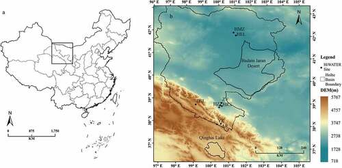
The study area is in Northwest China as shown in Figure 1a, covering the coordinate range between 96°E – 105.6°E, 36.45°N – 43°N, including the part of Qinghai, Gansu, Ningxia, Inner Mongolia provinces and part of Mongolia territory. The elevation in the study area ranges from 718 m to 5767 m, the southwest of the study area is part of the Tibetan Plateau, which is considered as the third pole of the earth, with an elevation from 3000 m to 5767 m. The black dotted box shows the extent of the second largest inland river basin in China, the Heihe River Basin (HRB). From the upstream to the downstream, the HRB includes multiple natural landscapes such as ice and snow, frozen soil, forest, grassland, river, lake, oasis, desert, and Gobi. The unique natural geographical environment makes HRB an important region for the study of inland river basin. At present, many scientific research and field experiments have been carried out in HRB, and accumulated abundant and valuable resources, which has laid a good scientific data foundation for basin ecological research (S. M. Liu et al., 2016; Xu et al., 2017). One objective is to evaluate remote sensing models, algorithms, and products through purposeful validation experiment (Duan et al., 2019; Jiang et al., 2015).

Figure 1. Map of the study area. Left panel shows the geographical location of the study area. Right panel shows a digital elevation model (DEM, m) overlaid with the measurement locations (points) and Heihe river basin boundary (dotted polygons). The nine black dots indicate ground-based LST measurement site from HiWATER.

FY3D MERSI-II data

FY-3D is loaded with ten sets of advanced remote sensing sensors. MERSI-II is one of the core sensors mounted on the FY-3D satellite. It is the world’s first sensor that can provide global daily 250 m resolution TIR data, and can seamlessly acquire true color images with a resolution of 250 m globally every day (H. Wang et al., 2019; Yan et al., 2021). MERSI-II TIR channels have been upgraded from three infrared windows of FY3A/B/C VIRR to 5. Table 1 shows the technical parameters of the MERSI-II TIR channels. Two adjacent long-wave TIR channels (24th band: 10.30–11.30 $\mu m$; 25th band: 11.50–12.50 $\mu m$) have similar interval setting with the 31st/32nd band of MODIS (31st band: 10.78–11.28 $\mu m$; 32nd band: 11.77–12.27 $\mu m$), which provides better opportunity to retrieve LST based on SW algorithm (H. Wang et al., 2019; Zheng et al., 2020). Figure 2 shows a comparison diagram of the spectral response functions of the 24th and 25th bands of MERSI-II and the 31st and 32nd bands of MODIS. The comparison showed certain differences in the spectral response functions of the two TIR channels of MERSI-II and MODIS. Hence, it is inappropriate to directly use the SW algorithm parameters by Qin et al. (2001b) to retrieve MERSI-II LST. In this study, we downloaded daily FY-3D MERSI-II level 1 (L1) multiband product data with a resolution of 250 m throughout the study area in 2019 to retrieve LST product.

Figure 2. The spectral response functions of MERSI-II and MODIS TIR channels.

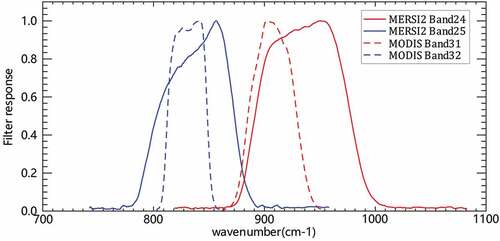
Table 1. The technical parameters of FY3D MERSI-II TIR channels.

Channels	Center Wavelength ($\mu m$)	spectral width ($nm$)	Spatial resolution (m)	SNR NE $\mathrm{\Delta }T$ (K)	Dynamic range (K)
20	3.8	180	1000	0.25	200–350
21	4.050	155	1000	0.25	200–380
22	7.2	500	1000	0.25	180–270
23	8.55	300	1000	0.25	180–300
24	10.8	1000	250	0.4	180–330
25	12.0	1000	250	0.4	180–330

Note: SNR NE $\mathrm{\Delta }T$ denotes the Noise equivalent temperature difference.

AQUA MODIS data

MODIS is an important sensor mounted on two sun-synchronous polar-orbiting satellites, namely, TERRA and AQUA. Its product data are mainly used for long-term global observation of land surface, biosphere, solid earth, atmosphere and ocean (S. Q. Yang et al., 2020; Sun et al., 2021). This study selected the LST product data from AQUA satellite (MYD11A1 V006) close to the overpass time of the FY3D satellite as the reference data, and used the inter-comparison method to evaluate the MERSI-II LST retrieval accuracy. MYD11A1 V006 is the sixth-generation MODIS LST product data retrieved by Wan (2014) using the generalized SW algorithm (Wan & Dozier, 1996) and day–night algorithm (Wan & Li, 1997), with spatial and temporal resolutions of 1 km and 1 d, respectively. Wan (2013) used the R-based method to verify MODIS LST using data from five bare soil sites in North Africa. The results showed that the average error of LST of 10 sets of data in 12 sets of verification data was within 0.6 K, the average error of 1 set of data was below 0.8 K, and the average error of LST of another group of data was less than 1.9 K. Duan et al. (2019) used the T-based method to verify the MODIS LST data using homogeneous site measurement data. The results showed that the RMSE value between MODIS LST and measured data during the day at most sites was relatively large ($>2K$). Moreover, the RMSE value between the night MODIS LST and measured data was less than 2 K.

HiWATER site data

Heihe Watershed Allied-Telemetry Experimental Research (HiWATER) is a multi-scale comprehensive observation experiment, in which satellite, aerial remote sensing and ground observation collaborate with each other. HiWATER is based on the Heihe River Basin’s established observation system and the results of the “Heihe Integrated Remote Sensing Joint Experiment” conducted from 2007 to 2009. This study selected the four-component radiation data of 2019 from nine ground observation stations of HiWATER to evaluate the accuracy of the MERSI-II LST product by T-based method (Song et al., 2020, 2016). Table 2 shows the information of the nine observing stations. The measured LST was observed by the CNR1/CNR4 four component radiometer set-up in the automatic weather station, with averaged values provided every 10 minutes and extracted for validation at FY3D overpass time. Eq.1was used to calculate the LST.

(1) $LST={\left[\frac{R_{up}-R_{down}\left(1-{\epsilon }_b\right)}{{\epsilon }_b\sigma }\right]}^{\frac{1}{4}}.$(1)

Table 2. The information of the four-component radiation site of HiWATER.

Site	Lat and Lon (${ }^{\circ })$	Altitude (m)	Land cover	Temporal resolution (minutes)
SDM	38.8555 ${ }^{\circ }\mathrm{N}$, 100.3722 ${ }^{\circ }\mathrm{E}$	1556	corn	10
ZY	38.9751 ${ }^{\circ }\mathrm{N}$, 100.4464 ${ }^{\circ }\mathrm{E}$	1460	wetland	10
AR	38.0473 ${ }^{\circ }\mathrm{N}$, 100.4643 ${ }^{\circ }\mathrm{E}$	3033	Subalpine mountain meadow	10
YK	38.0142 ${ }^{\circ }\mathrm{N}$, 100.2421 ${ }^{\circ }\mathrm{E}$	4148	Alpine meadow	10
HEL	41.9903 ${ }^{\circ }\mathrm{N}$, 101.1335 ${ }^{\circ }\mathrm{E}$	874	Populus euphratica and Tamarisk tamarix	10
HRS	38.827 ${ }^{\circ }\mathrm{N}$, 100.4756 ${ }^{\circ }\mathrm{E}$	1560	Artificial grass	10
HZZ	38.7659 ${ }^{\circ }\mathrm{N}$,100.3201 ${ }^{\circ }\mathrm{E}$	1731	desert	10
DSL	38.8399 ${ }^{\circ }\mathrm{N}$, 98.9406 ${ }^{\circ }\mathrm{E}$	3739	Alpine meadow	10
HMZ	42.1135 ${ }^{\circ }\mathrm{N}$, 100.9872 ${ }^{\circ }\mathrm{E}$	1054	desert	10

where $R_{up}$ is the surface upward long-wave radiation, $R_{down}$ is the atmospheric downward long-wave radiation at the surface, ${\epsilon }_b$ is the surface broadband emissivity, and its calculation method is discussed in Section 3.4, and $\sigma$ is the Stan–Boltzmann constant ($5.67\times {10}^{-8}W{m}^{-2}{K}^{-4}$).

The excellent LST verification site should be a homogeneous surface with small spatial heterogeneity from point scale to kilometer scale (Coll et al., 2012). Table 3 shows the standard deviation (STD) of the extracted Landsat8 LST in the $3\times 3$ and $10\times 10$ windows with each site as the center. It is used to evaluate the spatial heterogeneity of the surface of the nine ground stations on the MERSI-II 250 m and MODIS 1000 m scales. Except for the YK site, the STD values of Landsat8 LST in the regions of and $10\times 10$ at other sites were all below 1.06 K, it indicates that the surface spatial heterogeneity of HMZ, HEL, ZY, SDM, HRS, HZZ, and AR was small at scales of 250 m and 1000 m. Spatial heterogeneity of the DSL site was small at a scale of 250 m, but its spatial heterogeneity was relatively poor at a scale of 1000 m. The surface spatial heterogeneity of YK was poor at scales of 250 m and 1000 m. Hence, YK is not suitable for evaluating the remotely sensed LST product. By comparing the STD value of LST in the $3\times 3$ and $10\times 10$ windows, the STD value of LST in the $3\times 3$ window at each site was less than that in the $10\times 10$ window, thereby ideally reflecting the advantage of the LST products with 250 m resolution in small-scale surface environmental monitoring.

Table 3. The STD of the Landsat8 LST in the $3\times 3$ and $10\times 10$ windows with each site as the center.

Site Windows	STD(K)
	HMZ	HEL	DSL	ZY	SDM	HRS	HZZ	AR	YK
$3\times 3$	0.002	0.102	0.058	0.170	0.011	0.173	0.017	0.414	1.368
$10\times 10$	0.012	0.416	1.06	0.756	0.062	0.382	0.056	0.537	6.692

TIGR atmospheric profile data

The TIGR atmospheric profile database is composed of 2311 typical atmospheric profiles, which is widely used for the parameter simulation of LST and SST algorithms. TIGR atmospheric profile can be divided into five types: tropical atmospheric, mid-latitude summer, mid-latitude winter, polar summer, and polar winter profiles. The pressure value of the TIGR atmospheric profile is set from 1013hpa to 0.05hpa with 40 pressure layers. Each layer contains elevation, humidity, temperature, and ozone information.

Given that only clear sky is considered when retrieving LST, the cloud profile in the TIGR profile should be eliminated, and the criterion for determining cloud is that the relative humidity of any layer of the profile is above 90%, or that of two consecutive layers is over 85% (Galve et al., 2008; Tang et al., 2008). This study combined the determination conditions and characteristics of the study area, and selected 1132 clear sky atmospheric profile data from the mid-latitude summer profile as atmospheric input parameters.

Research methods

The SW Algorithm for FY3D MERSI-II

LST is the main research target of thermal infrared remote sensing application. Accurately retrieving LST is significant to the study of earth–atmosphere energy balance and ecosystems. Qin et al. (2001b) proposed the SW algorithm formula as follows:

(2) $T_s=A_0+A_1{T}_i-A_2{T}_j.$(2)

where $T_s$ is land surface temperature (K), $T_i$ and $T_j$ are the brightness temperatures (BT) of two thermal infrared bands with an atmospheric window in the range of 10–13 $\mu m$ (one is near 11 $\mu m$ and the other is near 12 $\mu m$), and $A_0$, $A_1$, and $A_2$ are the parameters of the SW algorithm.

ccording to radiative transfer theory, radiant energy received by satellites under clear sky conditions mainly comes from the earth’s surface and atmosphere, and is represented as follows:

(3) $B_{\lambda }\left(T_{\lambda }\right)=B_{\lambda }\left(T_s\right){\epsilon }_{\lambda }{\tau }_{\lambda }\left(\theta \right)+R_{\lambda }^{a\uparrow }\left(\theta \right)+\left(1-{\epsilon }_{\lambda }\right)R_{\lambda }^{a\downarrow }{\tau }_{\lambda }\left(\theta \right).$(3)

where $B_{\lambda }\left(T_{\lambda }\right)$ is the radiance received by the sensor with a wavelength of $\lambda$, $B_{\lambda }\left(T_s\right)$ is the radiance of the black-body when the surface temperature is $T_s$, ${\epsilon }_{\lambda }$ is the surface emissivity at the wavelength of $\lambda$, ${\tau }_{\lambda }$ indicates atmospheric transmittance in the direction from the target to the sensor, $R_{\lambda }^{a\uparrow }$ is the upwelling path radiances, and $R_{\lambda }^{a\downarrow }$ is the atmospheric downwelling path radiances. Qin et al. (2001b) used Eq.4 to approximate $R_i^{a\uparrow }\left(\theta \right)$ and $R_i^{a\downarrow }$, and held that using $T_a$ instead of $T_{a\downarrow }$ did not have considerable effect on the calculation result. Thus, Eq.3 can be simplified to Eq.5(5) $B_{\lambda }\left(T_{\lambda }\right)=B_{\lambda }\left(T_s\right){\epsilon }_{\lambda }{\tau }_{\lambda }\left(\theta \right)+\left(1-{\tau }_{\lambda }\left(\theta \right)\right)\left[1+\left(1-{\epsilon }_{\lambda }\right){\tau }_{\lambda }\left(\theta \right)\right]B_{\lambda }\left(T_a\right).$(5) :

(4a) $R_{\lambda }^{a\uparrow }=\left(1-{\tau }_{\lambda }\left(\theta \right)\right)B_{\lambda }\left(T_a\right).$(4a)

(4b) $R_{\lambda }^{a\downarrow }=\left(1-{\tau }_{\lambda }\left(\theta \right)\right)B_{\lambda }\left(T_{a\downarrow }\right).$(4b)

(5) $B_{\lambda }\left(T_{\lambda }\right)=B_{\lambda }\left(T_s\right){\epsilon }_{\lambda }{\tau }_{\lambda }\left(\theta \right)+\left(1-{\tau }_{\lambda }\left(\theta \right)\right)\left[1+\left(1-{\epsilon }_{\lambda }\right){\tau }_{\lambda }\left(\theta \right)\right]B_{\lambda }\left(T_a\right).$(5)

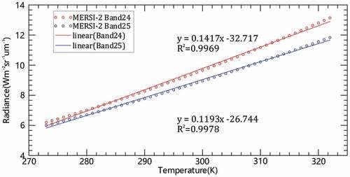
To continue solving Eq.5(5) $B_{\lambda }\left(T_{\lambda }\right)=B_{\lambda }\left(T_s\right){\epsilon }_{\lambda }{\tau }_{\lambda }\left(\theta \right)+\left(1-{\tau }_{\lambda }\left(\theta \right)\right)\left[1+\left(1-{\epsilon }_{\lambda }\right){\tau }_{\lambda }\left(\theta \right)\right]B_{\lambda }\left(T_a\right).$(5) , this study realizes the linearization of the Planck function, and constructed a close linear relationship between MERSI-II TIR radiance and LST. Figure 3 shows the relationship between the radiation and LST for MERSI-II 24th and 25th bands in the LST range of 273 K to 322 K. The linear fitting results (Eq.6a(6a) $B_{24}\left(T\right)=0.1417T_{24}-32.717R^2=\mathrm{0.9969.}$(6a) and Eq.6b)(6b) $B_{25}\left(T\right)=0.1193T_{25}-26.744R^2=\mathrm{0.9978.}$(6b) showed a strong linear relationship between the radiance and LST for MERSI-II TIR, and fitting accuracies $R^2$ were 0.9969 and 0.9978, respectively.

Figure 3. The linear relationship between the radiation and temperature for MERSI- II TIR.

(6a) $B_{24}\left(T\right)=0.1417T_{24}-32.717R^2=\mathrm{0.9969.}$(6a)

(6b) $B_{25}\left(T\right)=0.1193T_{25}-26.744R^2=\mathrm{0.9978.}$(6b)

By incorporating the linear fitting results into Eq.6, the LST retrieval Eq.7(7) $T_s=\left[C_{25}\left(B_{24}+D_{24}\right)-C_{24}\left(D_{25}+B_{25}\right)\right]/\left(C_{25}{A}_{24}-C_{24}{A}_{25}\right).$(7) for the 24th and 25th bands of MERSI-II can be derived as follows:

(7) $T_s=\left[C_{25}\left(B_{24}+D_{24}\right)-C_{24}\left(D_{25}+B_{25}\right)\right]/\left(C_{25}{A}_{24}-C_{24}{A}_{25}\right).$(7)

The algorithm parameters are shown in Eq.8:

(8a) $A_{24}=0.1417{\epsilon }_{24}{\tau }_{24}.$(8a)

(8b) $A_{25}=0.1193{\epsilon }_{25}{\tau }_{25}.$(8b)

(8c) $B_{24}=0.1417T_{24}+32.717{\epsilon }_{24}{\tau }_{24}-\mathrm{32.717.}$(8c)

(8d) $B_{25}=0.1193T_{25}+26.744{\epsilon }_{25}{\tau }_{25}-\mathrm{26.744.}$(8d)

(8e) $C_{24}=\left(1-{\tau }_{24}\right)\left[1+\left(1-{\epsilon }_{24}\right){\tau }_{24}\right]\times \mathrm{0.1417.}$(8e)

(8f) $C_{25}=\left(1-{\tau }_{25}\right)\left[1+\left(1-{\epsilon }_{25}\right){\tau }_{25}\right]\times \mathrm{0.1193.}$(8f)

(8g) $D_{24}=\left(1-{\tau }_{24}\right)\left[1+\left(1-{\epsilon }_{24}\right){\tau }_{24}\right]\times \mathrm{32.717.}$(8g)

(8h) $D_{25}=\left(1-{\tau }_{25}\right)\left[1+\left(1-{\epsilon }_{25}\right){\tau }_{25}\right]\times \mathrm{26.744.}$(8h)

Eq.8 shows that just the surface emissivity ${\epsilon }_{\lambda }$ and atmospheric transmittance ${\tau }_{\lambda }$ of the TIR channels of MERSI-II are needed to retrieve MERSI-II LST. Through linearization of the Planck function, while ensuring high LST retrieval accuracy, the unknown parameters of the original LST retrieval were reduced from three to two, thereby substantially reducing the complexity of the LST retrieval.

BT of the MERSI- II TIR bands

According to the calibration coefficient, the original DN value of the TIR channels can be converted into the radiation intensity value ($L_{\lambda }$). Thereafter, the equivalent black-body brightness temperature value ($T_{eff}$) can be calculated using the Planck equation. Lastly, the band brightness temperature correction parameter was used to convert $T_{eff}$ into the band blackbody brightness temperature.

(9) $L_{\lambda }=gain\cdot DN+offset.$(9)

(10) $T_{eff}=\frac{c_2\nu }{ln\left(1+c_1\nu /L_{\lambda }\right)}.$(10)

(11) $T_b=A\ast T_{eff}+B.$(11)

In Eq.9(9) $L_{\lambda }=gain\cdot DN+offset.$(9) , $gain$ is the gain value, $offset$ is the offset, and $DN$ is the gray value of the image. In Eq.10(10) $T_{eff}=\frac{c_2\nu }{ln\left(1+c_1\nu /L_{\lambda }\right)}.$(10) , $c_2$ and $c_1$ are constants, $c_2=2h{c}^2/{\lambda }^5$, and $c_1=hc/\left(K\lambda \right)$. In Eq.11(11) $T_b=A\ast T_{eff}+B.$(11) , A and B are band correction coefficients derived from the attribute variables in the MERSI-II L1 file.

Estimation of surface emissivity

Land surface emissivity (LSE) is one of the important input parameters in the process of LST retrieval. The error of LSE has a significant impact on the accuracy of LST. The retrieval algorithm of LSE can be roughly divided into three categories: Semi-Empirical Methods (SEMs), Multi-channel Temperature Emissivity Separation (TES), and Physically Based Methods (PBMs). SEM is the main algorithm to retrieve LSE in the process of LST retrieval (T. Song et al., 2015). This study is used the method of Qin et al. (2004) to estimate the emissivity of the natural surface.

Water has a high emissivity in the thermal infrared band, which is markedly like the black-body, and LSE of the water is set to 0.995. The ${\epsilon }_{building}$ and ${\epsilon }_{surface}$ of the two mixed pixels of urban and natural surfaces can be calculated using Eq.12(12) ${\epsilon }_{building}=P_v{R}_v{\epsilon }_v+\left(1-P_v\right)R_m{\epsilon }_m+d\epsilon .$(12) and Eq.13(13) ${\epsilon }_{surface}=P_v{R}_v{\epsilon }_v+\left(1-P_v\right)R_s{\epsilon }_s+d\epsilon .$(13) , respectively:

(12) ${\epsilon }_{building}=P_v{R}_v{\epsilon }_v+\left(1-P_v\right)R_m{\epsilon }_m+d\epsilon .$(12)

(13) ${\epsilon }_{surface}=P_v{R}_v{\epsilon }_v+\left(1-P_v\right)R_s{\epsilon }_s+d\epsilon .$(13)

where $P_v$ is the vegetation coverage, in which the calculation formula is shown in Eq.12(12) ${\epsilon }_{building}=P_v{R}_v{\epsilon }_v+\left(1-P_v\right)R_m{\epsilon }_m+d\epsilon .$(12) ; $NDV{I}_v$ and $NDV{I}_s$ represent the NDVI values of pure vegetation (0.75) and pure bare soil (0.05) pixels, respectively; $R_v$, $R_m$, and $R_s$ are the temperature ratios of vegetation, buildings, and bare soil respectively, the calculation formula of which is shown in Eq.14(14) $P_v=\frac{NDVI-NDV{I}_s}{NDV{I}_v-NDV{I}_s}.$(14) ; ${\epsilon }_v$, ${\epsilon }_m$, and ${\epsilon }_s$ are the LSE of vegetation, buildings, and bare soil, respectively, in which the values of the 24th band of MERSI-II are 0.9826, 0.965, and 0.974 respectively, and the values of the 25th band of MERSI-II are 0.987, 0.975, and 0.979 respectively (H. Wang et al., 2019); and $d\epsilon$ is the specific emissivity correction item, and its value is related to the surface coverage, when $P_v\le 0.5$, $d\epsilon =0.0038P_v$; when $P_v>0.5$, $d\epsilon =0.0038(1-P_v)$; when $P_v=0.5$, $d\epsilon =0.0019$; and when $P_v=0$ or 1, $d\epsilon =0$ (Qin et al., 2004; T. Song et al., 2015).

(14) $P_v=\frac{NDVI-NDV{I}_s}{NDV{I}_v-NDV{I}_s}.$(14)

(15a) $R_v=0.9332+0.0585P_v.$(15a)

(15b) $R_m=0.9886+0.1287P_v.$(15b)

(15c) $R_s=0.8802+0.1068P_v.$(15c)

Estimation of atmospheric transmittance

Atmospheric transmittance ($\tau$) is also one of the important input parameters of the SW algorithm (Qin et al., 2001b; Wan et al., 2004). Given that $\tau$ is difficult to obtain directly in real time (Wan, 2008), indirect estimation of $\tau$ by establishing the relationship between WVC and $\tau$ becomes a feasible method (Mao & Qin, 2004; Mao et al., 2005).

This study used 1132 TIGR clear sky atmospheric profile data as input parameters, and used MODTRAN4.0 to fit the relationship between WVC and $\tau$. Figure 4 shows the atmospheric transmittance and WVC scatter plot of the 24^th and 25^th bands of MERSI-II. The WVC values of the 1132 clear sky atmospheric profile data range from 0.06 $g/c{m}^2$ to 6.54 $g/c{m}^2$, atmospheric transmittance fitted by MODTRAN 4.0 was between 0.4 and 0.9, and atmospheric transmittance of the 24th and 25th bands of MERSI-II gradually decreased with an increase in WVC. Table 4 shows the fitting results of atmospheric transmittance and WVC of the 24th and 25th bands. The accuracies of the three fitting methods have small differences. The 24th band has the lowest linear fitting accuracy ($R^2=$ 0.974), and the cubic polynomial fitting has the highest accuracy ($R^2=$ 0.977). $R^2$ of the three fitting methods of the 25th band was 0.989. Through comparative analysis, this research used cubic polynomial to fit the relationship between atmospheric transmittance in two thermal infrared bands of MERSI-II and WVC.

Figure 4. The scatter plot between WVC and atmospheric transmittance simulated by MODTRAN4.0 of the 24th and 25th bands of MERSI-II.

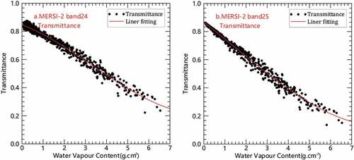
Table 4. The fitting results between WVC and atmospheric transmittance.

Fitting equation	Fitting accuracy
${\tau }_{24}=-0.090\omega +0.859$${\tau }_{25}=-0.1162\omega +0.8642$	$R^2=$ 0.974$R^2=$ 0.989
${\tau }_{24}=-0.0019{\omega }^2-0.081\omega +0.855$${\tau }_{25}=0.0037{\omega }^2-0.1332\omega +0.8723$	$R^2=$ 0.975$R^2=0.990$
${\tau }_{24}=0.0013{\omega }^3-0.0131{\omega }^2-0.058\omega +0.848$${\tau }_{25}=0.0008{\omega }^3-0.0034{\omega }^2-0.1186\omega +0.8677$	$R^2=$ 0.977$R^2=0.990$

The 18th band in the MERSI-II sensor is the water vapor absorption zone, and its center wavelength is 0.940 $\mu m$. The 15th band (center wavelength is 0.865 $\mu m$) and 19th band (center wavelength is 1.03 $\mu m$) are the two adjacent atmospheric window areas. Eq.16(16) $\tau =\rho \left(18\right)/\left(\rho \left(15\right)+\rho \left(19\right)\right).$(16) and Eq.17(17) $\omega ={\left[\frac{\alpha -ln\tau }{\beta }\right]}^2.$(17) are used to retrieve atmospheric transmittance and WVC, respectively. (Hu et al., 2011; H. Q. Yang et al., 2012; X. Wang et al., 2012).

(16) $\tau =\rho \left(18\right)/\left(\rho \left(15\right)+\rho \left(19\right)\right).$(16)

(17) $\omega ={\left[\frac{\alpha -ln\tau }{\beta }\right]}^2.$(17)

where $\omega$ is the atmospheric water vapor content ($g/c{m}^2$); $\tau$ is the atmospheric transmittance; and $\rho \left(15\right)$, $\rho \left(18\right)$, and $\rho \left(19\right)$ are the apparent reflectances of the 15th, 18th, and 19th bands, respectively, of the FY3D MERSI-II data. The values corresponding to the mixed pixels used in $\alpha$ and $\beta$ are 0.02 and 0.651, respectively.

Results and analysis

MERSI- II LST accuracy verification using the R-based method

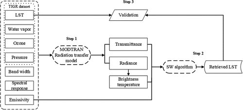
R-based method is a typical forward physical model, it simulates the TOA brightness temperature (BT) by inputting the initial parameters such as the satellite-derived LST, atmospheric profile data and the emissivity into the atmospheric radiative transfer model (Figure 5). During the simulation process, the input of the LST is continuously adjusted until the simulated TOA BT is consistent with the BT observed by the satellite sensor, and then the adjusted LST is considered as the real LST. Finally, the adjusted LST is compared with the LST retrieved by remote sensing to evaluate the error of the satellite-derived LST product.

Figure 5. Flowchart of accuracy evaluation of the SW algorithm.

On the assumption that the LSE is between 0.91 and 1.0 to include most land surface types, the atmospheric profile screened out in Section 2.5 and relevant information of MERSI-II TIR channels were applied to evaluate the absolute error of the re-fitting SW algorithm by using the atmospheric simulation model. The accuracy of the SW algorithm was characterized by bias, Mean Absolute Error (MAE) and Root Mean Square Error (RMSE) respectively (Eq.18(18) $Bias=\frac{{\sum }_{i=1}^n\left(Y_i-X_i\right)}{N}.$(18) , Eq.19(19) $MAE=\frac{{\sum }_{i=1}^n\left|Y_i-X_i\right|}{N}.$(19) and Eq.20)(20) $RMSE=\sqrt{\frac{{\sum }_{i=1}^n{\left(Y_i-X_i\right)}^2}{N}}.$(20) . 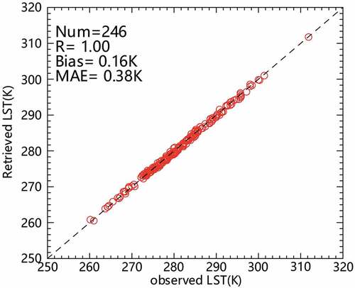Figure 6 shows the scatter plots of observed LST versus the LST retrieved by the atmospheric simulation model, which shows that the R value between $LS{T}_s$ and $LS{T}_t$ is close to 1.0, the Bias value is 0.16 K, and the MAE value is 0.38 K, indicating that the re-fitting SW algorithm proposed in this study has good accuracy and applicability.

(18) $Bias=\frac{{\sum }_{i=1}^n\left(Y_i-X_i\right)}{N}.$(18)

(19) $MAE=\frac{{\sum }_{i=1}^n\left|Y_i-X_i\right|}{N}.$(19)

(20) $RMSE=\sqrt{\frac{{\sum }_{i=1}^n{\left(Y_i-X_i\right)}^2}{N}}.$(20)

Figure 6. The scatter plots of observed LST versus the LST retrieved by the atmospheric simulation model.

Table 5 shows the absolute error of SW algorithm with different values and WVC values, which indicated that SW algorithm maintains good accuracy when WVC and $LS{T}_t$ change. The bias values between $LS{T}_s$ and $LS{T}_t$ is range from −0.179 K to 0.364 K, the MAE values range from 0.28 K to 0.487 K, and the RMSE values range from 0.332 K to 0.552 K. In addition, the absolute error of SW algorithm increases with the increase of $LS{T}_t$ and WVC.

Table 5. The absolute error of SW algorithm under different input conditions.

		LST<275 K	LST $\ge$ 275 K	All LST
W < 1.0 $g/c{m}^2$	Bias	−0.173 K	0.346 K	0.078 K
	MAE	0.289 K	0.401 K	0.346 K
	RMSE	0.332 K	0.491 K	0.419 K
W $\ge$ 1.0 $g/c{m}^2$	Bias	−0.153 K	0.364 K	0.323 K
	MAE	0.487 K	0.436 K	0.444 K
	RMSE	0.522 K	0.513 K	0.516 K
All Water vapor	Bias	−0.179 K	0.358 K	0.205 K
	MAE	0.327 K	0.424 K	0.400 K
	RMSE	0.373 K	0.506 K	0.472 K

MERSI- II LST accuracy verification using the inter-comparison method

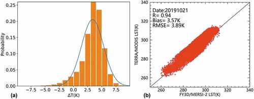
The inter-comparison method compares LST retrieved by the satellite with another remotely sensed LST product with good accuracy. This method does not require any ground measurement data and is a simple and feasible LST evaluation method (Coll et al., 2009; Gao et al., 2018). Figure 7 shows the spatial distribution of the MERSI-II LST(7a) and MODIS LST (7b) product on 21 October 2019. Moreover, Figure 8 indicates that the spatial distribution of MERSI-II LST on the north side of this study area was consistent with that of the MODIS LST products. The LST distribution map clearly distinguishes the Alxa Badain Jaran Desert. However, there were numerous low-value pixels in the MERSI-II LST product on the south side of the study area. These pixels were identified as cloud pixels in the MODIS LST product. The reason is that the cloud recognition based on the CDI index in this paper failed to identify and eliminate all cloud pixels in LST products. Figure 8 a and b shows the histogram and scatter plot of the differences between MERSI-II LST and MODIS LST, respectively. Figure 8a shows that the difference ($\mathrm{\Delta }T$) between MODIS LST and MERSI-II LST on 21 October 2019 was from −5 K to 7.5 K, and $\mathrm{\Delta }T$ was centrally distributed between 2.5 K and 5.0 K. Figure 8b shows that the bias values between MERSI-II LST and MODIS LST were 3.57 K and the RMSE value was 3.89 K, indicating that the MODIS LST values of many of the pixels were significantly higher than those of MERSI-II LST.

Figure 7. Product spatial distribution of MERSI- II LST(a) and MODIS LST(b) on 21 October 2019.

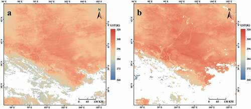
Figure 8. The Histogram(a) and scatter plot (b) of difference between MERSI- II LST and MODIS LST on 21 October 2019.

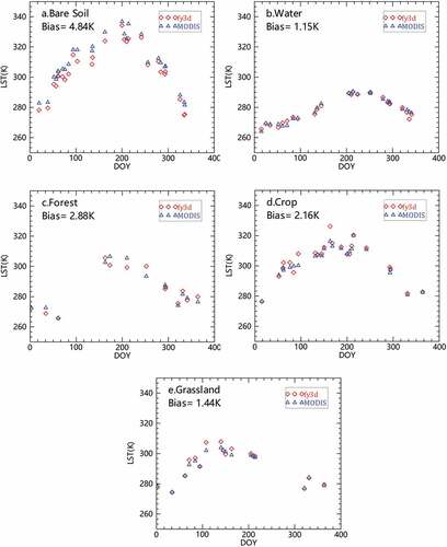
Figure 9 shows the LST value changes of MODIS and MERSI-II in (a) bare soil, (b) water, (c) Forest, (d) crop, and (e) grassland with time. MODIS LST and MERSI-II LST values have a highly consistent trend with time on different land cover types. Comparing Figure 9a and Figure 9e indicates that the value of $\mathrm{\Delta }T$ of MODIS and MERSI-II in the water was the smallest, the bias value was1.15 K, followed by grassland, in which the bias value was 1.44 K. The bias value of crops was 2.16 K, which is close to grassland. The bias value of Forest was 2.88 K. Meanwhile, the $\mathrm{\Delta }T$ in time series in bare soil was the largest, with a bias value of 4.84 K between LST of the two. The results show that the value of MERSI-II LST is lower than that of MODIS LST, and the $\mathrm{\Delta }T$ between two estimated LSTs is relatively small for homogeneous land surface, such as Water, Grassland and Cropland, while the $\mathrm{\Delta }T$ is large for heterogeneous land surface, particularly barren or sparsely vegetated land cover.

Figure 9. The LST values of MERSI- II and MODIS were distributed over time in bare soil (a), water body (b), forest land (c), crop (d) and grassland (e).

The inter-comparison method is usually used to evaluate the accuracy of LST product when there is a lack of site observation data, which reduces the cost of LST authenticity inspection. However, the uncertainty of the reference data itself, the difference of the observation angle, observation time, or the spatial resolution between the reference data and the comparison data make the accuracy evaluation results is relative rather than absolute (Li et al., 2016; J. Ma et al., 2017; Zhu et al., 2021).

MERSI-II LST accuracy verification using the T-based method

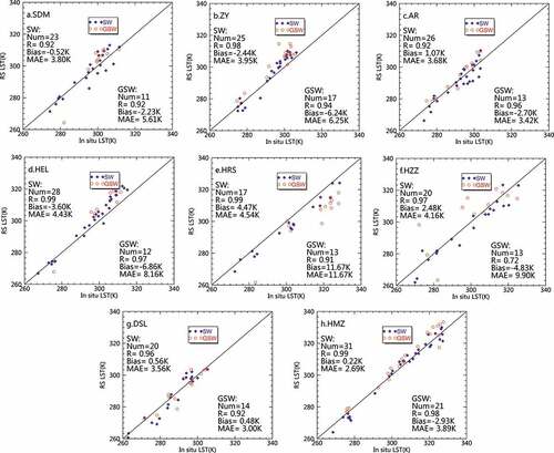
The T-based verification method is used to directly compare LST obtained by ground observation with LST retrieved by remote sensing through temporal–spatial–angle matching. This method is the most direct LST verification method (Duan et al., 2019). Figure 10 shows the scatter plots of the MERSI-II LST retrieved by SW and GSW algorithm (respectively called $LS{T}_s$ and $LS{T}_g$) and LST measured by (a) SDM, (b) ZY, (c) AR, (d) HEL, (e) HRS, (f) HZZ, (g) DSL, and (h) HMZ ($LS{T}_{st}$ t). The scatter plots show that the R value between MERSI-II $LS{T}_{\hspace{0.17em}}$ and $LS{T}_{st}$ at each site exceeded 0.92, and the R value passed the 0.01-level two-sided significance test, indicating a significant correlation between LST measured at the site and MERSI-II $LS{T}_s$. Bias value between the $LS{T}_{st}$ and MERSI-II $LS{T}_s$ was between −3.6 K and 4.4 K, and the MAE value was between 2.6 K and 4.54 K. The R value between MERSI-II $LS{T}_g$ and $LS{T}_{st}$ at each site exceeded 0.92, except for HZZ site. The bias between MERSI-II $LS{T}_g$ and $LS{T}_{st}$ was range from −6.25 K to 11.67 K. The high R value indicates that the time distribution of the MERSI-II LST product retrieved by the SW algorithm is consistent with the LST observed by the station. The relatively large MAE value also indicates a large error in the MERSI-II $LS{T}_g$ product.

Figure 10. The Scatter plots of MERSI-II LST and LST measured by AR(a), DSL(b), HEL(c), HMZ(d), HRS(e), HZZ(f), SDM(g), ZY(h) and all sites (i).

Table 6 shows the verification results of the MERSI-II LST retrieval accuracy under clear sky conditions. Except for March 2nd, the R values between MERSI-II LST and LST measured at the HiWATER site on the other days were between 0.93 and 0.99, the absolute value of bias was between 0.06 K and 1.47 K, and the MAE value was between 1.0 K and 2.66 K. Higher R value, lower Bias and MAE indicate that MERSI-II LST has higher accuracy under clear sky conditions, relatively, and can accurately characterize the thermal environment of the study area at a certain time. Figure 11 shows the overall accuracy assessment results of the eighth MERSI-II LST. R value between the eighth MERSI-II LST and site-measured LST was 0.99, bias value was −0.23 K, and MAE value was 2.03 K. Comparing Figures 10 and 11 shows that MAE value between LST measured by the site and MERSI-II LST is significantly reduced after removing some cloud pixels that account for a relatively large amount of data. This result indicates that cloud shadow and thin cloud pixels have immense impact on the accuracy of LST retrieval evaluated using the T-based method.

Figure 11. Overall accuracy evaluation results of MERSI-II LST products.

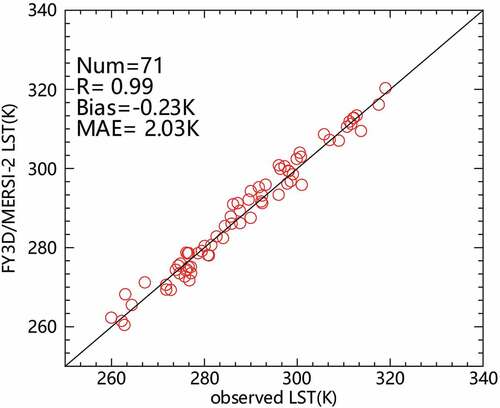
Table 6. The accuracy verification results of the MERSI-II LST under clear sky.

Time	correlation coefficient	Bias (K)	MAE (K)
January 2^nd	0.96**	0.32	1.84
March 2^nd	0.96**	1.69	3.26
May 16^th	0.99**	−0.06	1.0
July 24^th	0.97**	−0.07	1.95
October 6^th	0.99**	0.25	2.66
October 20^th	0.95**	−1.47	2.20
November 27th	0.95**	−0.21	1.43
December 1^st	0.93**	1.27	1.82

Note: ** indicates that there is a significant bilateral correlation at the level of 0.01

Discussion

Apart from the absolute error of the algorithm, LST retrieval error is also affected by numerous factors, such as WVC, $\tau$, and $\epsilon$. This research used Eq.20(20) $RMSE=\sqrt{\frac{{\sum }_{i=1}^n{\left(Y_i-X_i\right)}^2}{N}}.$(20) to evaluate the influence of the uncertainty of each parameter ($\mathrm{\Delta }x$) on LST retrieval error:

(21) $\mathrm{\Delta }{T}_S=\left|T_S\left(x+\mathrm{\Delta }x\right)-T_S\left(x\right)\right|.$(21)

where $\mathrm{\Delta }{T}_S$ is the error of LST retrieval, $x$ is the parameter affecting the accuracy of LST retrieval, $\mathrm{\Delta }x$ is the uncertainty of the parameter, $T_S\left(x+\mathrm{\Delta }x\right)$ and $T_S\left(x\right)$ represent LST value inverted when the parameter takes the values of $x+\mathrm{\Delta }x$ and $x$, respectively.

Influence of WVC on the accuracy of LST

Table 7 shows LST error obtained by changing WVC uncertainty ($\mathrm{\Delta }WVC$). In general, the average value of $\mathrm{\Delta }{T}_S$ increased with an increase in $\mathrm{\Delta }WVC$, and the average value of $\mathrm{\Delta }{T}_S$ was between 0 and 0.58 K. However, $\mathrm{\Delta }{T}_S$ does not follow this rule in all cases. When WVC was 3 $g/c{m}^2$, $\mathrm{\Delta }{T}_S$ increased with a negative growth of $\mathrm{\Delta }WVC$. When WVC was 4.2 $g/c{m}^2$, the value of (0.02 K) was smaller than that of $\mathrm{\Delta }{T}_S$ (0.11 K) when the WVC was 3.9 $g/c{m}^2$. Figure 12 shows the influence of ∆WVC on the accuracy of LST and MERSI-II’s 24th and 25th band atmospheric transmittances. When $\mathrm{\Delta }WVC$ was between −90% and 0, $\mathrm{\Delta }{T}_S$, $\mathrm{\Delta }{\tau }_{24}$, and $\mathrm{\Delta }{\tau }_{25}$ increased with an increase in $\mathrm{\Delta }WVC$. When was between 0 and 2.0 K, $\mathrm{\Delta }{\tau }_{24}$ and $\mathrm{\Delta }{\tau }_{25}$ were below 0.4. When $\mathrm{\Delta }WVC$ was between 0 and 90%, $\mathrm{\Delta }{T}_S$ did not increase with an increase in $\mathrm{\Delta }WVC$. When $\mathrm{\Delta }{T}_S$ was below 0.5, $\mathrm{\Delta }{\tau }_{24}$ and $\mathrm{\Delta }{\tau }_{25}$ were under 0.5. Kaufman and Gao (1992) confirmed that under cloud-free conditions, error of WVC retrieved by MODIS was between −13% and 13%. Given that MERSI-II and MODIS have similar TIR band settings, the sensitivity analysis of MERSI-II WVC can refer to the sensitivity analysis of MODIS (H. Wang et al., 2019). The preceding results indicate that LST and $\tau$ are not sensitive to WVC. Given that $\tau$ was calculated based on the WVC using three polynomial fitting calculations, this situation indirectly indicates that LST inverted by the SW algorithm was not sensitive to $\tau$.

Figure 12. The influence of ∆WVC on the accuracy of LST and MERSI-II’s 24th and 25th band atmospheric transmittances.

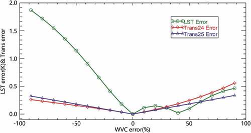
Table 7. The distribution of LST retrieval error with WVC uncertainty of SW algorithm.

WVC Error	WVC ($g/c{m}^2$)	$\mathrm{\Delta }{T}_S$(K)	WVC ($g/c{m}^2$)	$\mathrm{\Delta }{T}_S$(K)	WVC ($g/c{m}^2$)	$\mathrm{\Delta }{T}_S$(K)	Average $\mathrm{\Delta }{T}_S$ (K)
−40%	0.6	0.23	1.2	0.61	1.8	0.91	0.58
−30%	0.7	0.18	1.4	0.47	2.1	0.66	0.44
−20%	0.8	0.12	4.6	0.32	2.4	0.41	0.28
−10%	0.9	0.06	1.8	0.16	2.7	0.18	0.13
0	1.0	0	2.0	0	3.0	0	0
10%	1.1	0.06	2.2	0.17	3.3	0.11	0.11
20%	1.2	0.13	2.4	0.33	3.6	0.15	0.20
30%	1.3	0.20	2.6	0.49	3.9	0.11	0.27
40%	1.4	0.27	2.8	0.63	4.2	0.02	0.31

Influence of surface emissivity on the accuracy of LST

The uncertainty of surface emissivity ($\mathrm{\Delta }\epsilon$) is another key parameter of the SW algorithm. Figure 13 shows the effect of $\mathrm{\Delta }\epsilon$ on the accuracy of LST retrieval. When $\mathrm{\Delta }{\epsilon }_{24}$ and $\mathrm{\Delta }{\epsilon }_{25}$ changed equally between −0.0015 and 0.0015, LST retrieval error was between 0 and 0.68 K (Figure 14a); when ${\epsilon }_{25}$ remained unchanged (${\epsilon }_{25}=0.954$) and $\mathrm{\Delta }{\epsilon }_{24}$ changed from −0.0015 to 0.015, LST retrieval error was between 0 and 0.5 K (Figure 14b). When ${\epsilon }_{24}$ was unchanged (${\epsilon }_{24}=0.944$) and $\mathrm{\Delta }{\epsilon }_{25}$ was between −0.0015 and 0.015, LST retrieval error was between 0 and 1.2 K (Figure 14c). The preceding results showed that the LST retrieval error increased linearly with an increase in the absolute value of $\mathrm{\Delta }\epsilon$. Moreover, the change of $\mathrm{\Delta }{\epsilon }_{25}$ had a significantly greater impact on the accuracy of LST retrieval than $\mathrm{\Delta }{\epsilon }_{24}$.

Figure 13. The influence of surface emissivity uncertainty on LST accuracy under three different conditions. Fig. a show the surface emissivity of MERSI-II at 24th and 25th band with equal changes. Fig. b shows that 25th band remains unchanged and 24th band changes; Fig. c shows that 24th band remains unchanged and 25th band changes.

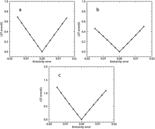
Figure 14. The influence of uncertainty of emissivity on LST retrieval accuracy under different emissivity in MERSI-II TIR band. Fig. a show the influence of ${\epsilon }_{24}$ uncertainty on LST retrieval accuracy when ${\epsilon }_{25}=0.954$, $0.944\le {\epsilon }_{24}\le 1.0$ . Fig. b shows the influence of ${\epsilon }_{25}$ uncertainty on LST retrieval accuracy when ${\epsilon }_{24}=0.944$, $0.954\le {\epsilon }_{25}\le 1.0$.

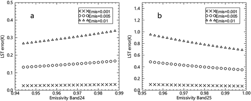
The numerical value of surface emissivity also affects the accuracy of LST retrieval. Figure 14 shows the effect of $\mathrm{\Delta }\epsilon$ on the accuracy of LST retrieval under different surface emissivity in the 24th and 25th bands of MERSI-II. Under the condition that ${\epsilon }_{25}=0.954$ was unchanged, ${\epsilon }_{24}$ changed from 0.944 to 1.0, when $\mathrm{\Delta }{\epsilon }_{24}=0.001$, LST retrieval error increased from 0.026 K to 0.035 K; when $\mathrm{\Delta }{\epsilon }_{24}=0.005$, LST retrieval error increased from 0.131 K to 0.177 K; and when $\mathrm{\Delta }{\epsilon }_{24}=0.01$, LST retrieval error increased from 0.267 K to 0.359 K. Under the condition that ${\epsilon }_{24}=0.944$ was unchanged, ${\epsilon }_{25}$ changed from 0.954 to 1.0; when $\mathrm{\Delta }{\epsilon }_{25}=0.001$, LST retrieval error decreased from 0.099 K to 0.071 K; when, LST retrieval error decreased from 0.486 K to 0.350 K; and when $\mathrm{\Delta }{\epsilon }_{25}=0.01$, LST retrieval error decreased from 0.952 K to 0.688 K. The preceding results show that under the same uncertainty, the greater the value of ${\epsilon }_{24}$, the greater the influence of $\mathrm{\Delta }{\epsilon }_{24}$ on LST retrieval error; and the greater the value of ${\epsilon }_{25}$, the smaller the influence of $\mathrm{\Delta }{\epsilon }_{25}$ on LST retrieval error.

Influence of cloud and snow pixels on LST

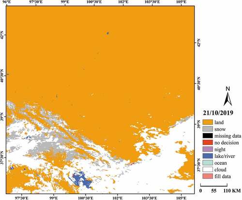
Figure 8a shows there were still numerous outlier pixels in the MERSI-II LST product, and these pixel values were significantly lower than LST value of the clear sky pixels. Figure 8b shows the MODIS LST product after effective cloud pixel recognition and removal. Comparing Figure 8 a and b, the low value areas of the MERSI-II LST product type correspond to the cloud pixels in MODIS LST. The acquisition time of the two LST products was similar, which completely shows that the abnormal value of MERSI-II LST was the pixel affected by cloud shadow and thin cloud. In addition, snow cover is also one of the factors that cannot be ignored to lead to abnormal value of MERSI-II LST pixels. By comparing Figure 8a and Figure 15, the differentiation constant pixels of MERSI-II LST product just corresponds to the snow pixel of MODIS snow cover product.

Figure 15. MODIS snow product data of the study area on 21 October 2019.

Conclusions

This study linearly simplified the Planck function based on the MERSI-II TIR band characteristics to re-fit the SW algorithm coefficients suitable for MERSI-II, and used the TIGR2000 data and MODTRAN4.0 model to fit the relationship between atmospheric transmittance and WVC. The objective is to obtain the atmospheric transmittance corresponding to the MERSI-II TIR band and realize the MERSI-II LST retrieval. Lastly, atmospheric profile data, MYD11A1 data and the four-component radiation data were used to evaluate the accuracy of the MERSI-II LST products using atmospheric simulate method, inter-comparison Method and T-based Method respectively.

The atmospheric simulate method shows that the R value between $LS{T}_s$ and $LS{T}_t$ is close to 1.0, the Bias value is 0.16 K, and the MAE value is 0.38 K, indicating that the re-fitting SW algorithm proposed in this study has good accuracy and applicability. The inter-comparison results show that the spatial distribution of MERSI-II LST and MODIS LST was relatively consistent, the difference LST (∆T) between MODIS and MERSI-II was between −5 K and 7.5 K, and ∆T was mainly distributed between 2.5 K and 5.0 K. Bias value was3.57 K, and RMSE value was 3.89 K. T-based method results show the R value between MERSI-II $LS{T}_s$ and the $LS{T}_{st}$ at each site exceeded 0.92, and R value passed the 0.01 level two-sided significance test. Bias value was between 3.6 K and 4.4 K, and MAE value was between 2.6 K and 4.54 K. the R value between MERSI-II $LS{T}_g$ and the $LS{T}_{st}$ at each site exceeded 0.92, except for HZZ site, and the bias value was between −6.25 K and 11.67 K. Higher R value, lower bias, and RMSE indicate that MERSI-II $LS{T}_s$ has higher accuracy at all stages and, relatively, can accurately characterize the thermal environment of the study area at a certain time. In comparison, the accuracy of $LS{T}_g$ is lower than that of $LS{T}_s$.

Author Contributions

Zhang Dejun guided the research process and completed the manuscript; Yang Shiqi completed the manuscript; Sun Liang provided algorithms, technical guidance, and modify the manuscript; Liu Xiaoran and Tang Shihao modified the manuscript and made specific comments; Zhu Hao, Ye Qinyu and Zhang Xinyu processed remote sensing data.

Disclosure statement

No potential conflict of interest was reported by the author(s).

Additional information

Funding

Supported by the Fengyun Application Pioneering Project of China (FY-APP-2021.0306), Science and Technology Department of Chongqing Municipality (cstc2020jcyj-msxmX1009), and Chongqing meteorological Department business technology project (YWJSGG-202106).

References

- Anderson, M. C., Norman, J. M., Kustas, W. P., Houborg, R., Starks, P. J., & Agam, N. (2008). A thermal-based remote sensing technique for routine mapping of land-surface carbon, water, and energy fluxes from field to regional scales. Remote Sensing of Environment, 112(12), 4227–4241. http://doi.org/10.1016/j.rse.2008.07.009
- Becker, F., & Li, Z. L. (1990). Towards a Local Split Window Method over Land Surface. International Journal of Remote Sensing, 11(3), 369–393. http://doi.org/10.1080/01431169008955028
- Cheng, Y. L., Wu, H., Li, Z. L., & Qian, Y. G. (2021). Retrieval and validation of the land surface temperature from FY-3D MERSI-II. National Remote Sensing Bulletin, 25(8), 1792–1807. http://doi.org/10.11834/jrs.20211302
- Chen, H. Y., Niu, Z., & Bi, B. (2013). A comparison of two split-window algorithm for retrieving land surface temperature from MODIS data. Remote Sensing Technology and Application, 28(2), 174–181. http://doi.org/10.11873/j.issn.1004-0323.2013.2.174
- Coll, C., Valor, E., Galve, J. M., Maria, M., Bisquert, M., García-Santos, V., Caselles, E., & Caselles, V. (2012). Long-term accuracy assessment of land surface temperature derived from the advanced along-track scanning radiometer. Remote Sensing of Environment, 116, 211–225. https://doi.org/10.1016/j.rse.2010.01.027
- Coll, C., Wan, Z. M., & Galve, J. M. (2009). Temperature-based and radiance-based validations of the V5 MODIS land surface temperature product. Journal of Geophysical Research Atmospheres, 114(D20), D20102. http://doi.org/10.1029/2009JD012038
- Dash, P., Gottsche, F. M., Olesen, F. S., & Fischer, H. (2005). Separating surface emissivity and temperature using two-channel spectral indices and emissivity composites and comparison with a vegetation fraction method. Remote Sensing of Environment, 96(1), 1–17. http://doi.org/10.1016/j.rse.2004.12.023
- Duan, S. B., Han, X. J., Huang, C., Li, Z. L., Wu, H., Qian, Y. G., Gao, M. F., & Leng, P. (2020). Land surface temperature retrieval from passive microwave satellite observations: State-of-the-art and future directions. Remote Sensing, 12(16), 2573. http://doi.org/10.3390/rs12162573
- Duan, S. B., Li, Z. L., Cheng, J., & Leng, P. (2017). Cross-satellite comparison of operational land surface temperature products derived from MODIS and ASTER data over bare soil surfaces. ISPRS Journal of Photogrammetry and Remote Sensing, 126, 1–10. http://doi.org/10.1016/j.isprsjprs.2017.02.003
- Duan, S. B., LI, Z. L., Li, H., Göttsche, F. M., Wu, H., Zhao, W., Leng, P., Zhang, X., & Coll, C. (2019). Validation of Collection 6 MODIS land surface temperature product using in situ measurements. Remote Sensing of Environment, 225, 16–29. http://doi.org/10.1016/j.rse.2019.02.020
- Duan, S. B., Li, Z. L., Tang, B. H., Wu, H., & Tang, R. L. (2014). Generation of a time-consistent land surface temperature product from MODIS data. Remote Sensing of Environment, 140, 339–349. https://doi.org/10.1016/j.rse.2013.09.003
- Ermida, S. L., Soares, P., Mantas, V., Göttsche, F. M., & Trigo, I. F. (2020). Google earth engine open-source code for land surface temperature estimation from the landsat series. Remote Sensing, 12(9), 1471. http://doi.org/10.3390/rs12091471
- Galve, J. M., Coll, C., Caselles, V., & Valor, E. (2008). An atmospheric radio sounding database for generating land surface temperature algorithms. IEEE Transactions on Geoscience and Remote Sensing, 46(5), 1547–1557. http://doi.org/10.1109/TGRS.2008.916084
- Gao, C. X., Shi, Q., Li, C. R., Tang, L. L., Ma, L. L., Qian, Y. G., Zhao, Y. G., & Ren, L. (2018). Evaluation of land surface temperature by comparing FY-3C/VIRR with TERRA/MODIS and MSG/SEVIRI data. International Journal of Remote Sensing, 40(1), 1–14. http://doi.org/10.1080/01431161.2018.1460514
- Hu, X. Q., Huang, Y. B., Lu, Q. F., & Zheng, J. (2011). Retrieving precipitable water vapor based on the Near-infrared data of FY-3A Satellite. Journal of Applied Meteorological Science, 22(1), 46–56. http://doi.org/10.11898/1001-7313.20110105
- Hulley, G. C., Ghent, D., Gttsche, F. M., Guillevic, P. C., Mildrexler, D. J., & Coll, C. (2019). Land surface temperature/. In G.C. Hulley & D. Ghent (Eds.), Taking the temperature of the earth: Steps towards integrated understanding of variability and change. [s.l.] (pp. 57–127). Elsevier. http://doi.org/10.1016/B978-0-12-814458-9.00003-4
- Hulley, G. C., Gttsche, F. M., Rivera, G., Hook, S. J., Freepartner, R. J., Martin, M. A., Cawse-Nicholson, K., & Johnson, W. R. (2021). Validation and quality assessment of the ECOSTRESS Level-2 land surface temperature and emissivity product. IEEE Transactions on Geoscience and Remote Sensing, 1–23. http://doi.org/10.1109/TGRS.2021.3079879
- Jiang, J. X., Li, H., Liu, Q. H., Wang, H. S., Du, Y. M., Cao, B., Zhong, B., & Wu, S. L. (2015). Evaluation of land surface temperature retrieval from FY-3B/VIRR data in an arid area of Northwestern China. Remote Sensing, 7(6), 7080–7104. http://doi.org/10.3390/rs70607080
- Jiang, G. M., Li, Z. L., & Nerry, F. (2006). Land surface emissivity retrieval from combined mid-infrared and thermal infrared data of MSG- SEVIRI. Remote Sensing of Environment, 105(4)(4), 326–340. http://doi.org/10.1016/j.rse.2006.07.015
- Jiang, J. X., Liu, Q. H., Li, H., & Huang, H. G. (2011). Split-window method for land surface temperature estimation from FY-3A/VIRR data. Geoscience & Remote Sensing Symposium. IEEE. http://doi.org/10.1109/igarss.2011.6048953
- Jimnez-Muoz, J. C., Cristobal, J., Sobrino, J. A., Sria, G., Ninyerola, M., & Pons, X. (2009). Revision of the single-channel algorithm for land surface temperature retrieval from Landsat thermal-infrared data. IEEE Transactions on Geoscience and Remote Sensing, 47(1), 339–349. https://doi.org/10.1109/tgrs.2008.2007125
- Jimnez-Muoz, J. C., & Sobrino, J. C. (2003). A generalized single-channel method for retrieving land surface temperature from remote sensing data. Journal of Geophysical Research-Atmospheres, 108(D22), 4688. http://doi.org/10.1029/2003JD003480
- Jimnez-Muoz, J. C., & Sobrino, J. A. (2010). A single-channel algorithm for land-surface temperature retrieval from ASTER data. IEEE Geoscience and Remote Sensing Letters, 7(1), 176–179. http://doi.org/10.119/LGRS.2009.2029534
- Kaufman, Y. J., & Gao, B. C. (1992). Remote Sensing of water vapor in the near IR from EOS/MODIS. IEEE Transactions on Geoscience and Remote Sensing, 30(5), 871–884. http://doi.org/10.1109/36.175321
- Lan, X. Y., Zhao, E. Y., Leng, P., Li, Z. L., Labed, J., Nerry, F., Zhang, X., & Shang, G. F. (2021). Alternative physical method for retrieving land surface temperatures from hyperspectral thermal infrared data: Application to IASI observations. IEEE Transactions on Geoscience and Remote Sensing, 1–12. http://doi.org/10.119/TGRS.2021.3056103
- Li, Z. L., Duan, S. B., Tang, B. H., Wu, H., Ren, H. Z., Yan, G. J., Tang, R. L., & Leng, P. (2016). Review of methods for land surface temperature derived from thermal infrared remotely sensed data. Journal of Remote Sensing, 20(5), 899–920. http://doi.org/10.11834/jrs.20166192
- Li, Z. L., Tang, B. H., Ren, H. Z., Yan, G. J., Wan, Z. M., Trigo, I. F., & Sobrino, J. A. (2013). Satellite-derived land surface temperature: Current status and perspectives. Remote Sensing of Environment, 131, 14–37. http://doi.org/10.1016/j.rse.2012.12.008
- Liu, Y. B., Hiyama, T., & Yamaguchi, Y. (2006). Scaling of land surface temperature using satellite data: A case examination on ASTER and MODIS products over a heterogeneous terrain area. Remote Sensing of Environment, 105(2), 115–128. http://doi.org/10.1016/j.rse.2006.06.012
- Liu, S. M., Xu, Z. W., Song, L. S., Zhao, Q. Y., Ge, Y., Xu, T. R., Ma, Y. F., Zhu, Z. L., Jia, Z. Z., & Zhang, F. (2016). Upscaling evapotranspiration measurements from multi-site to the satellite pixel scale over heterogeneous land surfaces. Agricultural and Forest Meteorology, 230-231, 97–113. http://doi.org/10.1016/j.agrformet.2016.04.008
- Mao, K. B., Li, S. M., Wang, D. L., Zhang, L. X., Wang, X. F., Tang, H. J., & Li, Z. L. (2011). Retrieval of land surface temperature and emissivity from ASTER1B data using a dynamic learning neural network. International Journal of Remote Sensing, 32(19), 5413–5423. http://doi.org/10.1080/01431161.2010.501043
- Mao, K. B., & Qin, Z. H. (2004). The Transmission model of atmospheric radiation and the computation of transmittance of MODTRAN. Geomatics & Spatial Information Technology, 27(4), 1–3. http://doi.org/10.1093/infdis/170.4.996
- Mao, K. B., Qin, Z. H., Shi, J., & Gong, P. (2005). A practical split-window algorithm for retrieving land-surface temperature from MODIS data. International Journal of Remote Sensing, 26(15), 3181–3204. http://doi.org/10.1080/01431160500044713
- Mao, K. B., Shi, J. C., Li, Z. L., & Tang, H. J. (2007). An RM-NN algorithm for retrieving land surface temperature and emissivity from EOS/MODIS data. Journal of Geophysical Research, 112(D21), D21102. http://doi.org/10.1029/2007JD008428
- Mao, K. B., Shi, J. C., Tang, H. J., Li, Z. L., Wang, X. F., & Chen, K. S. (2008). A Neural network technique for separating land surface emissivity and temperature from ASTER imagery. IEEE Transactions on Geoscience and Remote Sensing, 46(1), 200–208. https://doi.org/10.1109/tgrs.2007.907333
- Ma, X. L., Wan, Z. M., Moeller, C. C., Menzel, W. P., & Gumley, L. E. (2002). Simultaneous retrieval of atmospheric profiles, land-surface temperature, and surface emissivity from Moderate-Resolution Imaging Spectroradiometer thermal infrared data: Extension of a two-step physical algorithm. Applied Optics, 41(5), 909–924. http://doi.org/10.1364/AO.41.000909
- Ma, J., Zhou, J., Liu, S. M., & Wang, Y. (2017). Review on validation of remotely sensed land surface temperature. Advances in Earth Science, 32(6), 529–615. http://doi.org/10.11867/j.issn.1001-8166.2017.06.0615
- McMillin, L. M. (1975). Estimation of sea surface temperature from two infrared window measurements with different absorption. Journal of Geophysical Research, 80(36), 5113–5117. http://doi.org/10.1029/JC080i36p05113
- Neteler, M. (2010). Estimating daily land surface temperatures in mountainous environments by reconstructed MODIS LST data. Remote Sensing, 2(1), 333–351. http://doi.org/10.3390/rs1020333
- Nie, J., Ren, H. Z., Zheng, Y. T., Ghent, D., & Tansey, K. (2021). Land surface temperature and emissivity retrieval from nighttime middle-infrared and thermal-infrared Sentinel-3 images. IEEE Geoscience and Remote Sensing Letters, 18(5), 915–919. http://doi.org/10.1109/lgrs.2020.2986326
- Peres, L. F., & DaCamara, C. C. (2004). Land surface temperature and emissivity estimation based on the two-temperature method: Sensitivity analysis using simulated MSG/SEVIRI data. Remote Sensing of Environment, 91(3/4), 377–389. https://doi.org/10.1016/j.rse.2004.03.011
- Prata, A. J. (1993). Land surface temperature derived from the advanced very high-resolution radiometer and the along-track scanning radiometer: 1. Theory. Journal of Geophysical Research-Atmospheres, 98(D9), 16689–16702. http://doi.org/10.1029/93JD01206
- Prata, A. J., Caselle, V., Coll, C., Sobrino, J. A., & Ottl, C. (1995). Thermal remote sensing of land surface temperature from satellites: Current status and prospects. Remote Sensing Reviews, 12(3/4), 175–224. http://doi.org/10.1080/02757259509532285
- Qin, Z. H., Karnieli, A., & Berliner, P. (2001a). A mono-window algorithm for retrieving land surface temperature from Landsat TM data and its application to the Israel-Egypt border region. International Journal of Remote Sensing, 22(18), 3719–3746. http://doi.org/10.1080/01431160010006971
- Qin, Z. H., Li, W. J., Xu, B., Chen, Z. X., & Liu, J. (2004). The estimation of land surface emissivity for Landsat TM6. Remote Sensing for Land Resources, 3, 28–32. http://doi.org/10.3969/j.issn.1001-070X.2004.03.007
- Qin, Z. H., Zhang, M. H., & Arnon, K. (2001b). Split window algorithms for retrieving land surface temperature from NOAA-AVHRR data. Remote Sensing for Land Resources, 13(2), 33–42. http://doi.org/10.6046/gtzyyg.2001.02.07
- Sobrino, J. A., Jimnez-Muoz, J. C., & Paolini, L. (2004). land surface temperature retrieval from LANDSAT TM5. Remote Sensing of Environment, 90(4), 434–440. http://doi.org/10.1016/j.rse.2004.02.003
- Sobrino, J. A., Julien, Y., Atitar, M., & Nerry, F. (2008). NOAA-AVHRR orbital drift correction from solar zenithal angle data. IEEE Transactions on Geoscience and Remote Sensing, 46(12), 4014–4019. http://doi.org/10.1109/TGRS.2008.2000798
- Sobrino, J. A., Li, Z. L., Stoll, M. P., & Becker, F. (1996). Mulit-channel and Mulit-angle algorithms for estimating sea and land surface temperature with ATSR data. International Journal of Remote Sensing, 17(11), 2089–2114. https://doi.org/10.1080/01431169608948760
- Song, L. S., Bian, Z. J., Kustas, W. P., Liu, S. M., Xiao, Q., Nieto, H., Xu, Z. W., Yang, Y., Xu, T. R., & Han, X. J. (2020). Estimation of surface heat fluxes using multi-angular observations of radiative surface temperature. Remote Sensing of Environment, 239, 111674. http://doi.org/10.1016/j.rse.2020.111674
- Song, T., Duan, Z., Liu, J. Z., Shi, J. Z., Yan, F., Sheng, S. J., Huang, J., & Wu, W. (2015). Comparison of four algorithms to retrieve land surface temperature using landsat8 satellite. Journal of Remote Sensing, 19(3), 451–464. http://doi.org/10.11834/jrs.20154180
- Song, L. S., Liu, S. M., Kustas, W. P., Zhou, J., Xu, Z. W., Xia, T., & Li, M. S. (2016). Application of remote sensing-based two-source energy balance model for mapping field surface fluxes with composite and component surface temperatures. Agricultural and Forest Meteorology, 230-231, 8–19. http://doi.org/10.1016/j.agrformet.2016.01.005
- Sun, L., Chen, Z. X., Gao, F., Anderson, M., Song, L. S., Wang, L. M., Hu, B., & Yang, Y. (2017). Reconstructing daily clear-sky land surface temperature for cloudy regions from MODIS data. Computers & Geosciences, 105, 10–20. http://doi.org/10.1016/j.cageo.2017.04.007
- Sun, L., Gao, F., Xie, D. H., Anderson, M., Chen, R. Q., Yang, Y., Yang, Y., & Cheng, Z. X. (2021). Reconstructing daily 30 m NDVI over complex agricultural landscapes using a crop reference curve approach. Remote Sensing of Environment, 253, 112156. https://doi.org/10.1016/j.rse.2020.112156
- Sun, L., Liang, S. L., Yuan, W. P., & Chen, Z. X. (2013). Improving a Penman–Monteith evapotranspiration model by incorporating soil moisture control on soil evaporation in semiarid areas. International Journal of Digital Earth, 6(1), 134–156. https://doi.org/10.1080/17538947.2013.783635
- Sun, D. L., & Pinker, R. T. (2003). Estimation of land surface temperature from a Geostationary Operational Environmental Satellite (GOES-8). Journal of Geophysical Research-Atmospheres, 108(D11), 4326. https://doi.org/10.1029/2002jd002422
- Sun, L., Sun, R., Li, X. W., Liang, S. L., & Zhang, R. H. (2012). Monitoring surface soil moisture status based on remotely sensed surface temperature and vegetation index information. Agricultural and Forest Meteorology, 166-167, 175–187. http://doi.org/10.1016/j.agrformet.2012.07.015
- Tang, B. H., Bi, Y. Y., Li, Z. L., & Xia, J. (2008). Generalized split-window algorithm for estimate of land surface temperature from Chinese geostationary Fengyun meteorological satellite (FY-2C) data. Sensor, 8(2), 933–951. http://doi.org/10.3390/s8020933
- Wan, Z. M. (2008). New refinements and validation of the MODIS land-surface temperature/ emissivity products. Remote Sensing of Environment, 112(1), 59–74. http://doi.org/10.1016/j.rse.2006.06.026
- Wan, Z. M. (2013). New refinements and validation of the collection-6 MODIS land-surface temperature/emissivity product. Remote Sensing of Environment, 140, 36–45. http://doi.org/10.1016/j.rse.2013.08.027
- Wan, Z. M. (2014). New refinements and validation of the collection-6 MODIS land-surface temperature/emissivity product. Remote Sensing of Environment, 140, 36–45. http://doi.org/10.1016/j.rse.2013.08.027
- Wan, Z. M., & Dozier, J. (1996). A generalized split- window algorithm for retrieving land-surface temperature from space. IEEE Transactions on Geoscience and Remote Sensing, 34(4), 892–905. https://doi.org/10.1109/36.602541
- Wang, H., Mao, K. B., Mu, F. Y., Shi, J. C., Yang, J., Li, Z. L., & Qin, Z. H. (2019). A split window algorithm for retrieving land surface temperature from FY-3D MERSI-2 data. Remote Sensing, 11(18), 2083. http://doi.org/10.3390/rs11182083
- Wang, N., Tang, B. H., Li, C. R., & Li, Z. L. (2010). A generalized neural network for simultaneous retrieval of atmospheric profiles and surface temperature from hyperspectral thermal infrared data. IEEE International Geoscience and Remote Sensing Symposium, 1055–1058. Honolulu, USA: IEEE. http://doi.org/10.1109/igarss.2010.5651405.
- Wang, X., Zhao, D. Z., Su, X., Yang, J. H., & Ma, Y. J. (2012). Retrieving precipitable water vapor based on FY3A near-IR data. Journal of Infrared and Millimeter Waves, 31(6), 550–555. https://doi.org/10.3724/SP.J.1010.2012.00550
- Wan, Z. M., & Li, Z. L. (1997). A physics-based algorithm for retrieving land-surface emissivity and temperature from EOS/MODIS data. IEEE Transactions on Geoscience and Remote Sensing, 35(4), 980–996. http://doi.org/10.1109/36.602541
- Wan, Z. M., & Li, Z. L. (2008). Radiance-based validation of the V5 MODIS land-surface temperature product. International Journal of Remote Sensing, 29(17–18), 5373–5395. http://doi.org/10.1080/01431160802036565
- Wan, Z. M., Zhang, Y. L., Zhang, Q. C., & Li, Z. L. (2002). Validation of the land-surface temperature products retrieved from terra moderate resolution imaging spectroradiometer data. Remote Sensing of Environment, 83(1–2), 163–180. http://doi.org/10.1016/S0034-4257(02)00093-7
- Wan, Z. M., Zhang, Y. L., Zhang, Q. C., & Li, Z. L. (2004). Quality assessment and validation of the MODIS global land surface temperature. International Journal of Remote Sensing, 25(1), 261–274. https://doi.org/10.1080/0143116031000116417
- Xu, Z. W., Ma, Y. F., Liu, S. M., Shi, W. J., & Wang, J. M. (2017). Assessment of the energy balance closure under advective conditions and its impact using remote sensing data. Journal of Applied Meteorology and Climatology, 56(1), 127–140. http://doi.org/10.1175/JAMC-D-16-0096.1
- Yang, H. Q., Yin, Q., Zhou, H. M., & Ge, W. Q. (2012). Utilization of MATLAB to realize LST retrieval and thematic mapping from FY-3/MERSI data. Remote Sensing for Land & Resources, 4, 62–70. http://doi.org/10.6046/gtzyyg.2012.04.11
- Yang, S. Q., Zhang, D. J., Sun, L., Wang, Y. Q., & Gao, Y. H. (2020). Assessing drought conditions in cloudy regions using reconstructed land surface temperature. Journal of Meteorological Research, 34(2), 264–279. http://doi.org/10.1007/s13351-020-9136-4
- Yan, L., Hu, Y., Zhang, Y., Li, X. M., Dou, C. Y., Li, J., Shi, Y. D., & Zhang, L. J. (2021). Radiometric calibration evaluation for FY3D MERSI-II thermal infrared channels at Lake Qinghai. Remote Sensing, 13(3), 466. https://doi.org/10.3390/rs13030466
- Yin, C. L., Meng, F., & Yu, Q. R. (2020). Calculation of land surface emissivity and retrieval of land surface temperature based on a spectral mixing model. Infrared Physical and Technology, 108, 103333. https://doi.org/10.1016/j.infrared.2020.103333
- Zhang, D. J., Yang, S. Q., Wang, Y. Q., Sun, L., Gao, Y. H., Zhu, H., & Ye, Q. Y. (2021). Assessing drought conditions over cloudy regions based on reconstructed FY3C/VIRR LST. Journal of Natural Resources, 36(4), 1047–1061. http://doi.org/10.31497/zrzyxb.20210418
- Zheng, W., Chen, J., Tang, S. H., Hu, X. Q., & Liu, C. (2020). Fire monitoring based on FY-3D/MERSI-II far-infrared data. Journal of Infrared and Millimeter Waves, 39(1), 120–127. http://doi.org/10.11972/j.issn.1001-9014.2020.016
- Zhou, J., Zhan, W. F., Hu, D. Y., & Zhao, X. (2010). Improvement of mono-window algorithm for retrieving land surface temperature from HJ-1B satellite data. Chinese Geographical Science, 20(2), 123–131. http://doi.org/10.1007/s11769-010-0123-z
- Zhu, J. S., Ren, H. Z., Ye, X., Zeng, H., Nie, J., Jiang, C. C., & Guo, J. X. (2021). Ground validation of land surface temperature and surface emissivity from thermal infrared remote sensing data: A review. National Remote Sensing Bulletin, 25(8), 1538–1566. http://doi.org/10.11834/jrs.20211299