Spectral-based regression model for destriping of abnormal pixel values in PRISMA hyperspectral image

ABSTRACT

Hyperspectral imageries are often degraded by systematic sensor-based errors known as “striping noises”. This study implements a spectral-based regression algorithm from highly correlated consecutive bands, i.e. left band, right band or both, to model and reconstruct the abnormal pixel values, stripe noises, in various bands of PRISMA (PRecursore IperSpettrale della Missione Applicativa) imagery. The modeling performance was evaluated based on the statistical difference between the reconstructed images’ pixel values (reflectance) and their corresponding original pixel values. Results referred to the model’s high accuracy in R², RMSE, rRMSE and skewness in most bands $(0.9492<{\mathrm{R}}^2<0.9995;0.0008<RMSE<0.0254;0.0116\text{break}<rRMSE<0.5713-0.9280<skewness<0.2708$). Furthermore, the results indicated that the combination of both bands had higher accuracy and pixels’ homogeneity preservation compared to single-band modeling. Our findings suggested that the algorithm significantly depends on the spectral similarities between neighboring bands so that the higher spectral similarities lead to the higher model performance and vice versa. Subsequently, the minimum model performance was observed in band 143 due to lower spectral similarity, lower spectral correlation and higher wavelength differences with its adjacent right band. Finally, the study suggests that alongside other methods, our algorithm may be used as a reliable, straightforward and accurate alternative for destriping different Earth observation satellite imageries. Limitations of the proposed approach are also discussed.

KEYWORDS:

• Destriping
• hyperspectral image
• PRISMA
• spectral-based regression
• stripe noise

Introduction

Earth observation (EO) data are often contaminated with “striping noises”, also known as coherent noises, during image collection through scanning or pushbroom systems due to their different sensitivities, spectral response variation in the charge-coupled device (CCD), poor sensor radiometric calibration, etc. (Algazi & Ford, 1981; Behroozi et al., 2022; Gadallah et al., 2000; Kang et al., 2015; Lastri et al., 2015; B. Li et al., 2022; Pande-Chhetri & Abd-Elrahman, 2011). The coherence noises in scanning systems are generally periodic, whereas pushbroom noises are mainly non-periodic vertical stripes with different intensities (Lastri et al., 2015). However, both types of noises significantly degrade image quality, hindering the interpretability and the subsequent applications of imageries (Y. Chen et al., 2018; Pande-Chhetri & Abd-Elrahman, 2011; Y. J. Sun et al., 2019). These stripe noises are the most common and most prominent issues of satellite images that cause considerable biases in context analysis, feature analysis, image segmentation, image registration and geometric analysis of physical parameters (Kang et al., 2015; B. Li et al., 2022; Rakwatin et al., 2007). In order to better use EO data, destriping, i.e. correcting the stripe noises, plays a critical role in enhancing the image quality, improving signal-to-noise ratio (SNR) and accurately extracting features and related tasks (Tang et al., 2022). However, conventional and simple noise removal techniques may not be able to handle these stripe noises and preserve the radiometric homogeneity of the image. Therefore, it is essential to introduce and develop an efficient algorithm for correcting the stripe noises (destriping) before further analysis (classifications, segmentation, etc.).

To date, numerous methods have been proposed for stripe noise removal, which can be divided into three main approaches: (i) multi-source methods, (ii) single-source and (iii) hybrid methods (Darvishi Boloorani et al., 2008). The performance of these methods may vary depending on data type (single-band image, multispectral and hyperspectral image), stripe noise type and stripe noise intensity. Multisource algorithms such as local linear histogram matching (LLHM) correct the stripe noises using multisource imageries and other valuable datasets (Darvishi Boloorani et al., 2008; Roy et al., 2008; Scaramuzza et al., 2004; C. Zhang et al., 2007). These methods, which are mainly based on radiometric adjustments for spectral compensation between images (Maxwell et al., 2007), statistically assume that the input DNs of each sensor have similar statistical distributions (distribution function; mean and standard deviation) and then adjust these distributions by reference distribution (Acito et al., 2011; Gadallah et al., 2000; Q. Li et al., 2019; Qu et al., 2018). For example, local linear histogram matching was used to remove the strip noise in Landsat ETM+ (SLC-off) based on no-noise ETM+ (SLC-on) images (Scaramuzza et al., 2004). The algorithm showed a good performance in areas with the least temporal and seasonal variations and minimum land-cover changes; however, it is sensitive to input radiation, sung-glint variation and atmospheric conditions (Darvishi Boloorani et al., 2008). Another attempt developed a projection-transformation regression-based image reconstruction algorithm to handle the stripe noise in Landsat ETM+ (SLC-off) using earlier ETM+ (SLC-on) images (Darvishi Boloorani et al., 2008). However, this method was highly dependent on absolute transformation correction before algorithm implementation (Zeng et al., 2013). In addition, the main drawback of multi-source methods is that the assumption of similarity of the statistical distribution function of input digital numbers (DNs) may be violated in more complex surface structures. Nevertheless, these methods are more functional in images with a wide range of noise because it is difficult to obtain a multi-source information dataset (Bo Wang et al., 2017).

In single-source destriping methods, stripes are reconstructed based on neighborhood pixel interpolator or within pixel similarities from no-noise pixels in the image itself (Boloorani et al., 2008; Han et al., 2002; Qu et al., 2018; Bo Wang et al., 2017; Zeng et al., 2013). The thresholding algorithm based on horizontally traversal searching was then introduced to identify and detect abnormal pixel values (stripe noises) with DN values lower than immediate neighboring pixels (left and right pixels) and replaced by averaging (Goodenough et al., 2003; Han et al., 2002). However, traversal algorithm and thresholding are generally lengthy procedures, not time-efficient, and the thresholding varies among different images. Geostatistical destriping methods, such as ordinary kriging and especially variograms (Addink & Stein, 1999; Matheron, 1963; Pringle et al., 2009; C. Zhang et al., 2007), are also considered single-source algorithms that are used for destriping and showed reliable results (Boloorani et al., 2008; Darvishi Boloorani et al., 2008). However, the geostatistical destriping methods are not very successful on the heterogeneous land surfaces that may violate the basic intrinsic stationary assumption of the algorithm (Van der Meer, 2012; Zeng et al., 2013). To overcome the heterogeneity limitation of geostatistical techniques, Chen et al. (2011) introduced a Neighborhood Similar Pixel Interpolator (NSPI) to correct the stripe noises and restore the missed values in ETM+ (SLC-off) images with higher time and computational efficiency. Overall, destriping noisy images using the same data from the no-noise image achieves higher accuracy and reliability than other methods.

In hybrid models, which integrate two previous techniques, the stripe noises are corrected and removed utilizing the no-noise image itself. Still, the surface textures from other useful imageries (no-noise images) limit the interpolation (Darvishi Boloorani et al., 2008; Guo et al., 2020; Ma et al., 2022; Bo Wang et al., 2017; Bowen Wang et al., 2022; Wijedasa et al., 2012; K. Zhang et al., 2020). The coincident spectral algorithm, based on multi-scale segment mode to obtain the information from other valuable sources, was used for interpolating the spectral signatures and destriping (gap-filling) in Landsat 7 (ETM+-SLC off) images (Maxwell et al., 2007). Accordingly, Zhang et al. (2007) used the co-kriging geostatistical technique as a powerful tool for interpolating the miss-data in SLC-off EMT+ imageries. Although these techniques showed high accuracy for general or specific land-cover mapping, they are not suitable for per-pixel analysis such as landscape characterizations or impervious surface extractions (Maxwell et al., 2007). In addition, these methods are mainly based on image screening and characterization, which have low time efficiency and high computational load, and are not suitable for images with larger numbers of stripe noises (Bo Wang et al., 2017).

Although the aforementioned methods have been used to detect and correct stripe noises in various multispectral and hyperspectral images, in this context, to the best of our knowledge, destriping of the new available hyperspectral satellite imagery PRISMA (PRecursore IperSpettrale della Missione Applicativa) has received less attention with the stripe noises treated using more conventional methods such as spline smoothing-interpolation technique (Verrelst et al., 2021). PRISMA collects information by an imaging spectrometer with 233 spectral bands ranging from the visible near-infrared (VNIR) to the short-wave infrared (SWIR) spectrum through a pushbroom scanning mode. The configuration of hyperspectral image collection is somehow similar to traditional pushbroom scanners (Pande-Chhetri & Abd-Elrahman, 2011), and hence, the stripe noises (here referred to abnormal pixel values; Han et al., 2002) are also present in PRISMA images due to the sensor calibration (Goodenough et al., 2003) or electronic and optic facilities within the sensor (Tripathi & Garg, 2020). Furthermore, inappropriate calibration of detectors mainly causes striping artifacts in the imageries (Goodenough et al., 2003; Han et al., 2002). These abnormalities (abnormal pixel values) are usually manifested as continuous dark, or bright columns are apparent in VNIR and SWIR bands (e.g. bands 12, 56, 125, 127, etc.) with a width of three pixels.

As previously discussed, the main limitation of the above-mentioned algorithms is the high complexity in detection and correction of stripe noises, especially in hyperspectral images: therefore, to fill this gap, our novel and straightforward spectral-based regression algorithm aims to detect and correct abnormal pixel values (stripe noises) in the PRISMA dataset expected to process with lower computational costs. Subsequently, it preserves the original image homogeneity and continuity and minimizes the blurring effects from model implementation, differing from the abovementioned methods. In summary, state-of-the-art spectral-spatial methods rely on the spatial pixel similarities in a single band, and the other methods are based on the use of multisource data (auxiliary data, Landsat SLC-on, etc.), which are mainly complex, time-consuming and sensitive to the texture of the pixels that might inherently differ and often require images not available of the target scene (due to cloud cover, temporal differences, etc.). Our proposed spectral-based regression algorithm, benefitting from the highly correlated neighbouring bands (left, right or both), offers a straightforward, reliable and accurate tool for predicting and reconstructing abnormal pixel values in hyperspectral imageries. Another advantage of our method compared to the previous methods is that the use of spatial pixel similarities and pixel neighbourhood similarities may lead to image inconsistency at the location of the abnormal pixel values because the adjacent pixels may have different intrinsic properties (different surface texture, different surface object, class, etc.), leading to lower performance of the model in the destriping of stripe noise.

The remainder of this paper is organized as follows. The Materials and methods section describes the main characteristics of PRISMA dataset, and the spectral-based linear regression algorithm is formulated and explained in detail. In the Results section, we present the results of the model implementation to demonstrate the effectiveness of the algorithm, the Discussion section discusses the main finding in our paper and finally in the Conclusion section, we conclude our work.

Materials and methods

PRISMA hyperspectral sensor

PRISMA is a mission developed and launched (on 22 March 2019) by the Italian Space Agency (ASI), obtaining images based on users’ demand for a particular area of interest (Loizzo et al., 2019). PRISMA mission offers a wide range of applications from environmental monitoring to resource management, such as forest mapping, mineral explorations, mining, water quality, shallow water bathymetry, glacier ice retrieval, etc. (Alevizos et al., 2022; Bohn et al., 2022; Verrelst et al., 2021). PRISMA is based on prisms as a dispersive technology that transforms the input radiation on a 2D focal plane detector, which collects information through pushbroom scanning mode using an imaging spectrometer in a continuum of 233 spectral bands ranging from visible near-infrared (VNIR; 400 nm) to short-wave infrared (SWIR; 2500 nm) with spectral resolution lower than 12 nm, orbit mean altitude of 615 km (Alevizos et al., 2022; Loizzo et al., 2019; Vangi et al., 2021) and revisiting periods of 29 days. It combines hyperspectral sensors and a panchromatic camera with Ground Sample Distance (GSD) of 30 and 5 m, respectively (Loizzo et al., 2019). The PRISMA provides the ability to obtain, downlink and archive images from hyperspectral and panchromatic bands in a total of 200,000 square kilometers per day within the desired target area defined in the following coordinates: 180°W-180°E to 70°S-70°N (Loizzo et al., 2019). A comprehensive explanation of the PRISMA sensor and its technical specifications are provided in Coppo et al. (2019) and Loizzo et al. (2019). The main characteristic of the sensor is tabulated in Table 1. For the purpose of this study, a PRISMA-L2D (level 2D-HD5 file) cloud-free dataset comprising of 30*30 km scene for Dublin, Ireland, was acquired (date: 20 July 2021) from the PRISMA portal (https://prisma.asi.it) for destriping and abnormal pixel value reconstruction. PRSIMA-L2D is orthorectified and atmospherically corrected (at-surface reflectance; Vangi et al., 2021). Dublin city is geographically situated between 53° 21’ 0.5040” N latitude and 6°15’ 58.1580”W longitude in the eastern region of Ireland (see Figure 1). The selected scene from Dublin city comprises various land-use/land-cover units including vegetation, wet soil, river, built area, etc.

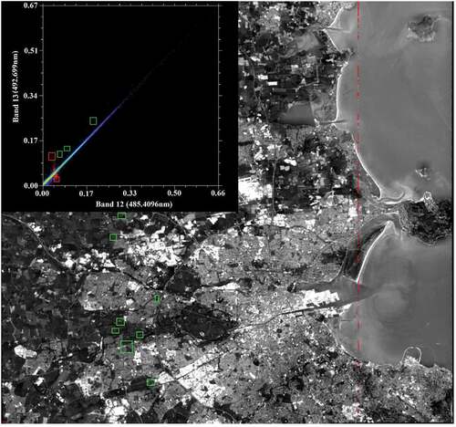
Figure 1. Geographical location of study area (Dublin, Ireland) covered by PRISMA hyperspectral imagery shown in true color composite (R: 623.1971 nm, G: 522.9162 nm, B: 470.9489 nm) obtained on 20 July 2021.

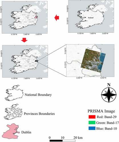
Table 1. Main technical specifications of PRISMA payload.

Orbit altitude	615 km
Swath/field of view	30 km/2.77◦
Ground sample distance	Hyperspectral: 30 m PAN: 5 m
Spatial pixels	Hyperspectral: 1000 PAN: 6000
Pixel size	Hyperspectral: 30 × 30 µm PAN: 6.5 × 6.5 µm
Spectral range	VNIR: 400–1010 nm (66 bands) SWIR: 920–2500 nm (173 bands) PAN: 400–700 nm 615 km 30 km/2.77◦
Spectral sampling interval (SSI)	≤12 nm
Spectral width	≤12 nm
Spectral calibration accuracy	±0.1 nm
Radiometric quantization	12 bit
VNIR signal to noise ratio (SNR)	>200:1
SWIR SNR	>100:1
PAN SNR	>240:1
Absolute radiometric accuracy	Better than 5% PRISMA

Methods

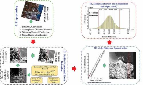
The destriping of abnormal pixel values in the PRISMA dataset was performed in four stages, including (1) PRISMA preprocessing; (2) outlier/abnormal pixel value detection based on Gaussian model; (3) abnormal pixel value prediction using spectral-based ordinary least square regression algorithm; and (4) model validation and comparison.

A schematic of the proposed methodology is provided and represented in Figure 2. The detailed explanation of each step is as follows:

Figure 2. Flowchart of adopted methodology for destriping of PRISMA dataset.

PRISMA preprocessing

Before model implementation, it is necessary to preprocess the PRISMA image to avoid any bias during the modeling. The preprocessing was implemented as follows:

PRISMA conversion: the PRISMA image was converted into a suitable format by the specific R package “prismaread” developed for importing and converting the PRISMA hyperspectral cubes to the desirable formats (Busetto & Ranghetti, 2020) .

“Atmospheric channels” removal: we filtered out and removed the channels (bands) that were spectrally located in the atmospheric absorption regions, mainly water vapor absorption channels (Verrelst et al., 2021), and since they did not provide valuable surface information (402.4402–456.3773 nm; 1349.5990–1480.6201 nm; 1793.6891–1984.5479 nm; and 2349.5752–2496.8740 nm).

“Window-Channels” selection: in this step, we considered only the filtered-out bands, and among these, the contaminated bands with stripe noises (abnormal pixel values), visually recognizable, were investigated for destriping model implementation. The statistics of the contaminated bands with stripe noises and their adjacent bands and the proximity to the atmospheric absorption channels are calculated and presented in Table S1.

Definition and detection of outlier/abnormal pixels

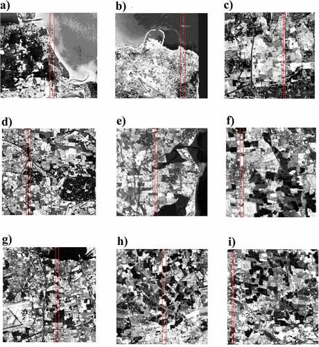
Abnormal pixel values occur as a brighter or darker columns (stripes) of pixels in the grayscale values compared to their adjacent pixels and are easily recognizable from the image texture in the VNIR and SWIR spectrum (in the available PRISMA image, bands No. 13, 21, 56, 61, 66, 137, 143, 189 and 196 were recognized as contaminated). For better visualization of the abnormal pixel values, we rotated the image with the angle of −15.7345 for Dublin city and considered each stripe as a vertical column of abnormal pixels. Thus, the start and end points of the abnormal pixel values remain in a column so that the stripe columns can be quickly visualized across all bands and images (see Figure 3), which ultimately facilitates the comparison between the spectral signature of abnormal pixel values and neighbouring pixels.

Figure 3. Observed stripes (within the dashed red rectangle) in different bands of PRISMA dataset as dark and bright columns. a, b, c, d, e, f, g, h, i are subset images from bands 13, 21, 56, 61, 66, 137, 143, 189, and 196, respectively.

Since hyperspectral images collect information over a wide range of spectra with very narrow bands (Licciardi & Chanussot, 2018; Seydi & Hasanlou, 2017), successive bands in the images show a very strong spectral correlation (Behroozi et al., 2022; Goetz, 1992; Q. Li et al., 2019). Benefiting from this point, we collected the spectral signatures from abnormal pixel locations and neighbouring pixels (non-noisy pixels) in different land-cover classes (vegetation and non-vegetation classes) to investigate the spectral behaviour of the abnormal pixel values compared to their adjacent pixel values in various bands (see Figure 4). Figure 4 represents the spectral behavior of vegetation and non-vegetation (built area; band 189) classes (three pixels in each band belong to the same land-cover classes, in bands 13 (492.6999 nm; vegetation class), 56 (897.9865 nm; vegetation class), 137 (1736.2556 nm; vegetation class), and 189 (2190.8354 nm; built-area)) varying from VNIR to SWIR spectrum. As the figure clearly shows, although all three pixels (left pixel, noisy pixel and right pixel) belong to the same classes with similar spectral behavior, the abnormal pixel values do not flow in the same behavior (abnormality clearly shown in the figure red ellipses). This spectral behavior deviation can be used to indicate abnormal pixel values. Hence, it can be inferred that the spectral signature analysis can be used as a reliable and accurate tool for abnormal pixel identification and characterization. Furthermore, the high spectral correlation behavior between the noisy band and its adjacent bands is represented in Figure 5.

Figure 4. Example of spectral signatures (at surface reflectance) collected in the location of abnormal pixels from a noisy pixel (light blue line) and its neighboring pixels, right pixel (pink line) and left right (green line), in four different bands: (a) band 13 (492.6999 nm; vegetation class) and its represented zoom of reflectivities in a narrower wavelength range (b); (c) band 56 (897.9865; vegetation class) and its represented zoom (d); (e) band 137 (1736.2556 nm; vegetation class) and its represented zoom (f); (g) band 189 (2190.8354; built-area) and its represented zoom (h).

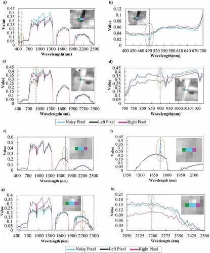
Figure 5. Example of scatter plot between the noisy band 13 and the neighboring band 12. The graph refers to the high spectral correlation between the two bands and, based on the visual interpretation of the scatter plot, the abnormal pixels (highlighted in red colors; abnormal pixels are a subset of the outliers) and the outliers (in green color; some spread green pixels are inside the green boxes) were highlighted in the graph.

Subsequently, the spectral signatures from the pixels of neighboring bands (left and right bands or a combination of both) were utilized for abnormal pixel prediction and reconstruction in the contaminated bands with stripe noises. This study adopted a first-order spectral-based polynomial equation to efficiently fit a linear model based on ordinary least square method (OLSM) between the noisy band and its neighboring bands (left, right or both) in PRISMA imagery. The mathematical formulation of OLSM is explained in detail as follows:

Ordinary least squares (OLS) is a type of linear least square algorithm, which uses a linear function for predicting the relationship between dependent and independent variables by minimizing sum of the square errors. OLS method is a strong and robust algorithm which can be effectively used in predicting missing pixels in different applications in remote sensing, which is suited for predicting missing data in various datasets. In general, regressive interpolation methods (linear, multiple and iterative) are a robust tool with higher performance than other models for estimating the variable dataset with a high degree of correlation (Abdul Jabar et al., 2016; Guo et al., 2020; Jiang et al., 2009; Ma et al., 2022; Bowen Wang et al., 2022; K. Zhang et al., 2020), especially in hyperspectral dataset. Let’s assume that there is a high linear correlation between the bands with abnormal pixel values ($PRIMA.S_{i\left(i=1,2,..,N\right)}$) and the corresponding pixels values in its adjacent bands ($PRIMA.\mathrm{A}\mathrm{d}{\mathrm{j}}_{i\left(i=1,2,..,N\right)}$), the linear regression using OSLM can be formulated as follows:

(1) $\left[\begin{array}{c}\begin{array}{c}PRIMA.{\mathrm{S}}_1\\ PRIMA.{\mathrm{S}}_2\\ PRIMA.{\mathrm{S}}_3\end{array}\\ ⋮\\ PRIMA.{\mathrm{S}}_N\end{array}\right]=\left[\begin{array}{c}\begin{array}{cc}1& PRIMA.\mathrm{A}\mathrm{d}{\mathrm{j}}_1\\ 1& PRIMA.\mathrm{A}\mathrm{d}{\mathrm{j}}_2\\ 1& PRIMA.\mathrm{A}\mathrm{d}{\mathrm{j}}_3\end{array}\\ \begin{array}{cc}⋮& ⋮\\ 1& PRIMA.\mathrm{A}\mathrm{d}{\mathrm{j}}_N\end{array}\end{array}\right]\left[\begin{array}{c}a\\ b\end{array}\right]+\left[\begin{array}{c}\begin{array}{c}{e}_1\\ e_2\\ e_3\end{array}\\ ⋮\\ e_N\end{array}\right]$(1)

(2) $\left[\begin{array}{c}\hat{a}\\ \hat{b}\end{array}\right]=({\left[\begin{array}{c}\begin{array}{cc}1& PRIMA.\mathrm{A}\mathrm{d}{\mathrm{j}}_1\\ 1& PRIMA.\mathrm{A}\mathrm{d}{\mathrm{j}}_2\\ 1& PRIMA.\mathrm{A}\mathrm{d}{\mathrm{j}}_3\end{array}\\ \begin{array}{cc}⋮& ⋮\\ 1& PRIMA.\mathrm{A}\mathrm{d}{\mathrm{j}}_N\end{array}\end{array}\right]}^T\ast \left[\begin{array}{c}\begin{array}{cc}1& PRIMA.\mathrm{A}\mathrm{d}{\mathrm{j}}_1\\ 1& PRIMA.\mathrm{A}\mathrm{d}{\mathrm{j}}_2\\ 1& PRIMA.\mathrm{A}\mathrm{d}{\mathrm{j}}_3\end{array}\\ \begin{array}{cc}⋮& ⋮\\ 1& PRIMA.\mathrm{A}\mathrm{d}{\mathrm{j}}_N\end{array}\end{array}\right]{)}^{-1}\ast {\left[\begin{array}{c}\begin{array}{cc}1& PRIMA.\mathrm{A}\mathrm{d}{\mathrm{j}}_1\\ 1& PRIMA.\mathrm{A}\mathrm{d}{\mathrm{j}}_2\\ 1& PRIMA.\mathrm{A}\mathrm{d}{\mathrm{j}}_3\end{array}\\ \begin{array}{cc}⋮& ⋮\\ 1& PRIMA.\mathrm{A}\mathrm{d}{\mathrm{j}}_N\end{array}\end{array}\right]}^T\ast \left[\begin{array}{c}\begin{array}{c}PRIMA.{\mathrm{S}}_1\\ PRIMA.{\mathrm{S}}_2\\ PRIMA.{\mathrm{S}}_3\end{array}\\ ⋮\\ PRIMA.{\mathrm{S}}_N\end{array}\right]$(2)

(3) $\left[\begin{array}{c}\begin{array}{c}\widehat{e_1}\\ \widehat{e_2}\\ \widehat{e_3}\end{array}\\ ⋮\\ \widehat{e_N}\end{array}\right]=\left[\begin{array}{c}\begin{array}{cc}1& PRIMA.\mathrm{A}\mathrm{d}{\mathrm{j}}_1\\ 1& PRIMA.\mathrm{A}\mathrm{d}{\mathrm{j}}_2\\ 1& PRIMA.\mathrm{A}\mathrm{d}{\mathrm{j}}_3\end{array}\\ \begin{array}{cc}⋮& ⋮\\ 1& PRIMA.\mathrm{A}\mathrm{d}{\mathrm{j}}_N\end{array}\end{array}\right]\left[\begin{array}{c}\hat{\alpha }\\ \hat{b}\end{array}\right]-\left[\begin{array}{c}\begin{array}{c}PRIMA.{\mathrm{S}}_1\\ PRIMA.{\mathrm{S}}_2\\ PRIMA.{\mathrm{S}}_3\end{array}\\ ⋮\\ PRIMA.{\mathrm{S}}_N\end{array}\right]$(3)

where N is the total pixel numbers (m*n); a, b are model coefficients; $\hat{a}$, $\hat{b}$ are estimated model coefficients; $e_{i\left(i=1,2,\dots ,N\right)}$ is the modelling residual; and $\widehat{e_{i\left(i=1,..,N\right)}}$ are the estimated error values which mainly include abnormal pixel values.

To identify and eliminate outliers (mainly randomly spread in the image) and abnormal pixel values (pixels’ abnormality relative to the adjacent pixels as a subset of outliers), we adopted the OLSM as mentioned above between the noisy band and adjacent bands (left and right bands). Then, the Gaussian thresholding function (Equation 4(4) $G\left(x;{\mu }_{\lambda },{\sigma }_{\lambda }\right)=\frac{1}{\sigma \sqrt{2\pi }}{e}^{-\frac{1}{2}{\left(\frac{x-\mu }{\sigma }\right)}^2}$(4) ), as one of the most efficient methods in OLSM residual analysis, was performed for hypothesis testing and error estimation based on confidence intervals (Folks & Chhikara, 1978). Specifically, the pixel values out of 99.9% confidence interval (µ-3.291σ~µ + 3.291σ), as an optimal interval, were considered as potential outliers, including abnormal pixels, and were removed from all bands to perform the spectral-based linear regression.

(4) $G\left(x;{\mu }_{\lambda },{\sigma }_{\lambda }\right)=\frac{1}{\sigma \sqrt{2\pi }}{e}^{-\frac{1}{2}{\left(\frac{x-\mu }{\sigma }\right)}^2}$(4)

where ${\mu }_{\lambda }$ and ${\sigma }_{\lambda }$ are the mean value and standard deviations for each individual band estimated from Gaussian fitting over all pixels in the specific target bands (bands with stripe noises).

Spectral-adjacency OLSM regression implementation

As mentioned above, the implementation of the proposed destriping algorithm is based on a spectral-adjacency OLSM. The basic idea behind spectral-OLSM regression (statistical-based analysis) is to predict and reconstruct the abnormal pixel values in the imagery with the help of adjacent no-noisy bands in the image. The spectral-adjacency regression algorithm was implemented as follows.

After removing the outliers and abnormal pixel values (described above), the remaining pixels of each band and its consecutive bands’ pixels were divided into training (70% of total image pixels) and validation (30% of total image pixels) datasets. Next, the OLS model was again performed on the training data (70% of total image pixels) between the filtered image and its neighboring bands (left, right and both; Jiang et al., 2009; Yin, Mariethoz, Sun et al., 2017; Zeng et al., 2013) to derive the regression coefficients. The derived coefficients from the models (left, right and both) were used to predict three images ($PRISM{A}_{pL,R,Avg}$), i.e. the contaminated band with stripe noises, based on neighboring bands.

In the last step, the abnormal pixel values and outliers from the original pixels were replaced by the estimated pixel value from the models (predicted images), and the final image (reconstructed image with replaced abnormal pixel values) was derived. Therefore, the final image contains the original image characteristics, original image characteristics are preserved, and the predicted (replaced) abnormal pixel values. The model performance was evaluated from the validation dataset, described in detail in the next section.

Predicting abnormal pixel values from the noisy band and its adjacent bands (left, right and both) was performed using the pixel values in the training as follows:

(5) $PRISM{A}_{pL}=\beta { }_0+\beta { }_1\ast BandL$(5)

(6) $PRISM{A}_{pR}=a{ }_0+a{ }_1\ast BandR$(6)

where $PRM{A}_{pL}$ and $PRISM{A}_{pR}$ are predicted noisy band values (at-surface reflectance) based on the left (L subscript) and right (R subscript) neighboring bands; $\beta { }_0$ and $a{ }_0$ are the model intercept; and $\beta { }_1$, $a{ }_1$ are the model slope for left and right bands (Band L and Band R).

In the next step, the regression-based model was fitted based on both images. The above equations can be modified if both images are used (combined and averaged) in the model building as follows:

(7) $PRISM{A}_{Avg}={\gamma }_0+{\gamma }_1\ast \frac{\left(BandL+BandR\right)}{2}$(7)

where $PRISM{A}_{avg}$ is averaged predicted noisy band based on the combination of the left and the right neighbor bands and ${\gamma }_0,{\gamma }_1$ are model intercept and slope, respectively.

In addition, it is important to note that the slopes and intercepts in the three models (left, right and both) were derived from all the no-noise pixels of the contaminated bands and their adjacent bands individually. Therefore, the derived coefficients (slope and intercept) were only used for predicting those pixels that were out of the confidence interval (Equation 1(1) $\left[\begin{array}{c}\begin{array}{c}PRIMA.{\mathrm{S}}_1\\ PRIMA.{\mathrm{S}}_2\\ PRIMA.{\mathrm{S}}_3\end{array}\\ ⋮\\ PRIMA.{\mathrm{S}}_N\end{array}\right]=\left[\begin{array}{c}\begin{array}{cc}1& PRIMA.\mathrm{A}\mathrm{d}{\mathrm{j}}_1\\ 1& PRIMA.\mathrm{A}\mathrm{d}{\mathrm{j}}_2\\ 1& PRIMA.\mathrm{A}\mathrm{d}{\mathrm{j}}_3\end{array}\\ \begin{array}{cc}⋮& ⋮\\ 1& PRIMA.\mathrm{A}\mathrm{d}{\mathrm{j}}_N\end{array}\end{array}\right]\left[\begin{array}{c}a\\ b\end{array}\right]+\left[\begin{array}{c}\begin{array}{c}{e}_1\\ e_2\\ e_3\end{array}\\ ⋮\\ e_N\end{array}\right]$(1) ), i.e. the abnormal pixel values, while preserving the original image characteristics without pixel values alteration outside the noisy ones.

Model validation and comparison

Model evaluation is critical to infer the model’s capability to reconstruct the abnormal pixel values and select the most suitable reconstructed image. The algorithm performance for three reconstructed images (from the left, right and both adjacent bands) was assessed using a validation dataset. This validation dataset (30% of total image pixels) is collected from the target bands without outliers/abnormal pixel values (i.e. outliers/abnormal pixel values are excluded). The modeling performance was evaluated based on the difference (rate of similarity) between the pixel values of predicted images from the modeling and their corresponding pixel values in the test image (validation dataset). The performance was assessed using different statistical criteria, including a histogram model of the error, coefficient of determination (R²), root mean square error (RMSE), relative root mean square error (rRMSE) and skewness index. Let us consider $PRISM{A}_{\lambda \left(i,j\right)}^p$ (L, R or both) and $PRISM{A}_{\lambda \left(i,j\right)}^o$ as the predicted and original images, respectively, and $\overline{PRISM{A}_{\lambda \left(i,j\right)}^o}$ and $\overline{PRISM{A}_{\lambda \left(i,j\right)}^p}$ as their mean values over the N(m × n) pixels of the image, the R², RMSE and skewness can be derived as follows:

(8) $\mathrm{R}\mathrm{M}\mathrm{S}{\mathrm{E}}_{\lambda }=\sqrt{\frac{1}{m\times n}\sum _{i=1}^m\sum _{j=1}^n{\left(PRISM{A}_{\lambda \left(i,j\right)}^p-PRISM{A}_{\lambda \left(i,j\right)}^o\right)}^2}$(8)

where $PRISM{A}_{\lambda \left(i,j\right)}^o$ is the filtered test pixels from original band in PRISMA that are not contaminated with stripe noises for each wavelength (band: $\lambda$). Accordingly, $PRISM{A}_{\lambda \left(i,j\right)}^p$ is the corresponding predicted pixel for each wavelength (band: λ), and $i,j$ refer to row and column of pixels’ location (test and predicted).

Smaller values of RMSE indicate the smaller rate of prediction error and higher rate of model performance (Yin, Mariethoz, McCabe et al., 2017).

(9) ${\mathrm{R}}_{\lambda }^2={\left(\frac{{\sum }_{i=1}^m{\sum }_{j=1}^n\left(PRISM{A}_{\lambda \left(i,j\right)}^p-\overline{PRISM{A}_{\lambda \left(i,j\right)}^p}\right)\left(PRISM{A}_{\lambda \left(i,j\right)}^o-\overline{PRISM{A}_{\lambda \left(i,j\right)}^o}\right)}{\sqrt{{\sum }_{i=1}^N{\left(PRISM{A}_{\lambda \left(i,j\right)}^p-\overline{PRISM{A}_{\lambda \left(i,j\right)}^p}\right)}^2{\sum }_{i=1}^N{\left(PRISM{A}_{\lambda \left(i,j\right)}^o-\overline{PRISM{A}_{\lambda \left(i,j\right)}^o}\right)}^2}}\right)}^2$(9)

$R^2$ is the measure of consistency between destriped image (reconstructed) and original noisy image ranging in the [0,1] interval (Yin, Mariethoz, McCabe et al., 2017).

Higher $R^2$, closer to 1, refers to the higher rate of similarity and consistency between two images and better performance of algorithms, whereas lower values of $R^2$ indicate the poor performance of model in reconstructing the image.

Because the RMSE may differ in different bands (VIS, NIR, SWR) and the reflectance values are affected by the different spectral signature of different land covers (Yin, Mariethoz, McCabe et al., 2017), we also computed relative root mean square error (rRMSE) to evaluate the model’s performance, using Equation 8(8) $\mathrm{R}\mathrm{M}\mathrm{S}{\mathrm{E}}_{\lambda }=\sqrt{\frac{1}{m\times n}\sum _{i=1}^m\sum _{j=1}^n{\left(PRISM{A}_{\lambda \left(i,j\right)}^p-PRISM{A}_{\lambda \left(i,j\right)}^o\right)}^2}$(8) .

(10) $rRMS{E}_{\lambda }=\frac{RMS{E}_{\lambda }}{\overline{PRISM{A}_{\lambda }^o}}$(10)

where $rRMS{E}_{\lambda }$ is the computed rRMSE for individual bands.

Furthermore, the performance of our model was evaluated from the histogram statistics of the error and of the error skewness using the following equation:

(11) $\widetilde{m_{3\lambda }}=\frac{1}{\left(N\right)\ast \delta {{ }_i^o}^3}\ast \sum _{i=1}^N{\left(PRISM{A}_i^p-\overline{PRISM{A}_i^o}\right)}^3$(11)

where ${\delta }_i^o$ is the standard deviation of original PRISMA dataset (after abnormal pixel and outlier removal). Skewness, a third moment of the mean is a critical measure of asymmetry (normality) of the distribution (error; Bartels et al., 2006; David, 1953; Davies, 1947). $\widetilde{m_3}$ closer to 0 refers to the perfect normality and symmetric distribution (Bartels et al., 2006). Negative values of $\widetilde{m_3}$ indicate the left tail skewness, whereas positive values represent the right-tail skewness. The model implementation and evaluation were performed for individual contaminated bands with stripe noises.

Results

The spectral-based regression algorithm for destriping PRISMA dataset (Dublin city) was performed on nine contaminated bands with stripe noises (bands 13, 21, 56, 61, 66, 137, 143, 189 and 196) using training data which is 70% of total pixels excluding outliers and abnormal pixel values. The regression coefficients (slope and intercept) for each model are derived, and the results are presented and explained below.

Results from linear regression modeling of VNIR bands (13; 492.6999 nm, 21; 554.5646 nm, 56; 897.9865 nm, 61; 942.9579 nm, and 66; 988.4116 nm)

Overall, 989*1069 pixels were analyzed in band 13, after rotation and clipping, equal to 1,057,241 pixels, of which 2233 pixels were outliers including abnormal pixels, 755,416 were training pixels, and 299,592 were test pixels. Almost the same pixel statistics were found in all other bands. The spectral-based regression algorithm for abnormal pixel value (stripe) prediction and reconstruction was implemented in band 13 (492.6999 nm) with the aid of its consecutive left and right bands (band 12; 485.4096 nm, and band 14; 500.1372 nm and the combination of both bands), and the results are elucidated in Figure 6(a–f).

Figure 6. Results of abnormal pixel value prediction using spectral-based linear regression between band 13 and neighboring bands. (a) Destriping based on right band (band 14); (b) Reconstructed band (final image) based on band 14; (c) Destriping based on left band (band 12); (d) Reconstructed band base on band 12; Reconstructed band (final image) based on band 14; (e) Destriping based on both bands (12, 14); and (f) Reconstructed band based on both bands (12, 14).

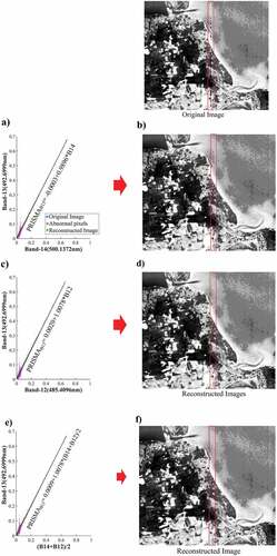
Figure 6a,c,e explicates that the model perfectly fitted the linear relationship between the abnormal pixel values in band 13 and adjacent bands and accurately predicted them using the high spectral correlations between bands (spectral similarities). From a visual perspective (see Figure 6b,d,f samples of the reconstructed scenes), by comparing the pixels in the original noisy band and the reconstructed pixels (stripes within the red dash-line in Figure 6b,d,f), it is clear that the algorithm adequately predicted the abnormal pixel values and reconstructed the noisy band well in three models. In addition, it is spotted that the algorithm effectively restored the image texture continuity in the stripe noise pixel’s location. Figure 7(a,b) clearly shows the high performance of the algorithm in destriping of abnormal pixel values using both images (high-zoom sample section was selected to highlight the model effectiveness).

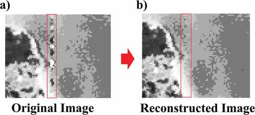
Figure 7. A sample section (high-zoom) of reconstructed image shows the effectiveness of the model in the destriping of abnormal pixel values in band 13 using a combination of both band (bands 12 and 14).

The noticeable difference between the reconstructed image, i.e. the final image with replaced (predicted) abnormal pixel values and outliers, and the original image is more pronounced in the northern and southern parts of the scene, where the abnormal pixels (bright or dark) mainly belong to the waterbody and vegetation classes (approximately three-pixel widths): the algorithm reliably predicted and replaced the abnormal pixels while preserving the pixels’ continuity and homogeneity.

For more evaluation, different statistical criteria (R², RMSE, skewness and error histogram) were used to assess and compare the models’ performance by the three regressions (left, right and both), and the results are presented in Table 2 and Figure 8(a–c). Table 2 and Figure 8(a–c) compare the statistical inference and histogram of the errors (difference between observed and predicted) for modeling based on bands 12, 14 and combinations of both.

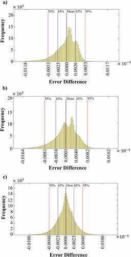
Figure 8. Histograms of the errors (difference between observed and the predicted values) for reconstructed image (band 13) based on its consecutive bands. (a) Histogram errors for modeling based on band 12, (b) histogram errors for modeling based on band 14 and (c) histogram errors for modeling based on both bands (12–14).

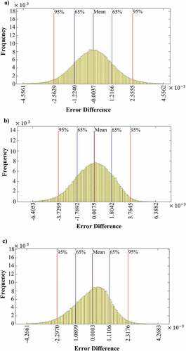
Table 2. Comparison of the spectral-based linear regression model in destriping PRISMA images based on the left band, right band and combination of both, using the coefficient of determination (R²), root mean square (RMSE), skewness index and mean of error values.

Criteria/band no.	Band 13 (492.6999 nm)	Band 21 (554.5646 nm)	Band 56 (897.9865 nm)	Band 61 (942.9579 nm)	Band 66 (988.4116 nm)	Band 137 (1736.2556 nm)	Band 143 (1793.6891 nm)	Band189 (2190.8354 nm)	Band 196 (2245.2136 nm)
RMSE left	0.0021	0.0013	0.0051	0.0254	0.0045	0.0045	0.0076	0.0039	0.0038
RMSE right	0.0015	0.0015	0.0034	0.0126	0.0046	0.0039	0.0461	0.0043	0.0043
RMSE both	0.0012	0.0008	0.0028	0.0166	0.0035	0.0019	0.0239	0.0033	0.0029
R^2 left	0.9924	0.9974	0.9985	0.9492	0.9990	0.9973	0.9895	0.9960	0.9956
R^2 right	0.9962	0.9964	0.9993	0.9876	0.9990	0.9980	0.6126	0.9952	0.9943
R^2 both	0.9974	0.9988	0.9995	0.9779	0.9994	0.9995	0.8956	0.9971	0.9973
rRMSE L	0.0689	0.0232	0.0214	0.0987	0.0184	0.0288	0.0560	0.0406	0.0411
rRMSE R	0.0453	0.0273	0.0141	0.0604	0.0180	0.0262	0.5713	0.0449	0.0490
rRMSE both	0.0389	0.0154	0.0116	0.0711	0.0138	0.0122	0.2210	0.0345	0.0325
Skewness left	−0.2673	−0.2454	−0.6055	−0.7168	0.2708	−0.2001	−0.1764	0.0921	−0.0716
Skewness right	0.0493	0.2035	−0.2294	−0.2594	−0.0384	−0.1559	−0.2603	0.1755	0.0209
Skewness both	−0.3956	−0.1284	−0.9280	−0.7145	0.1630	−0.0487	−0.1567	0.1396	−0.7160

The statistical comparison revealed that the algorithm performed very well with a relatively high coefficient of determination (R²), low rRMSE and RMSE and low skewness index in all three cases (left, right and both) with R² = 0.9924, 0.9962 and 0.9974; RMSE = 0.0021, 0.0015 and 0.0012; rRMSE = 0.0689, 0.0453 and 0.0389; and skewness = −0.2673, 0.0493 and −0.3956 for the left band, right band and combination of both, respectively. Besides, it was observed that the model has slightly showed better results in destriping the image using the right band (14) than the left band (12) with higher R², lower RMSE, lower rRMSE and lower skewness (0.9962, 0.0015, 0.0493 and 0.0453). However, it is also perceived that the algorithm slightly outperformed the other two models using a combination of both consecutive bands (bands 12 and 14) with higher coefficient of determination (R² = 0.9974) and a lower RMSE (0.0012) and lower rRMSE (0.0389). The histogram error analysis demonstrated a fairly symmetrical shape (normally distributed) of the errors in three models, with a better performance for the third model (both bands), referring to a relatively equal overestimation and underestimation of the predicted pixel values (Figure 8a–c). Besides, the predicted pixel values in the third model had lower error values compared to the other two models (left and right), ranging between [(−1.0899, 1.1106) × 10⁻³] at 65% confidence intervals and [(−2.2970, 2.3176) × 10⁻³] at 95% confidence interval (Figure 8a-c). Although the skewness value in modeling based on both images (left and right bands) was slightly higher, this could be due to the average of the model errors from the left and right bands, which deviated the error histogram towards the model with higher error values.

The model evaluation showed a relatively similar performance in most cases using the adjacent band approach for the contaminated bands with stripe noises including 21, 56, 61 and 66. For instance, the spectral-based destriping algorithm in band 56 (897.9865 nm) showed outstanding results in all three models, with slight outperformance of the model using both bands (bands 57; 908.6440 nm and 55; 887.2659 nm) ($R_{55}^2<R_{57}^2<R_{55,57}^2;rRMS{E}_{55,57}<rRMS{E}_{57}<rRMS{E}_{55};\text{break}RMS{E}_{55,57}<RMS{E}_{57}<RMS{E}_{55};$ (see Table 2). Therefore, the algorithm accurately predicted the abnormal pixel values by the three models with low overestimation, underestimation rate and very low range of error values (Figures 9a,c,e, and 10 a–-c). Figure (9b,d,f) illustrates the sample section of the reconstructed images on different land surfaces in the abnormal pixel’s location. The model’s effectiveness is clearly visible throughout the scene, especially in the center and northern regions inside the red box, mainly belonging to the vegetation and built-area classes. Overall, the algorithm reconstructed the final image (where the abnormal pixel values and outliers are replaced with the new predicted values) with high accuracy, maintaining the original feature of the image well. The modeling results for bands 21, 61 and 66 are provided in Table 2 and illustrated in Figures S1(a–f), S2(a–c), S3(a–f), S4(a–c), S5(a–f) and S6(a–c).

Figure 9. Results of abnormal pixel value prediction using spectral-based linear regression between band 56 and neighboring bands. (a) Destriping based on right band (band 57); (b) Reconstructed band based on band 57; (c) Destriping based on left band (band 55); (d) Reconstructed band based on band 55; (e); Destriping based on both bands (bands 55, 57); and (f) Reconstructed band based on both bands (band 55, 57).

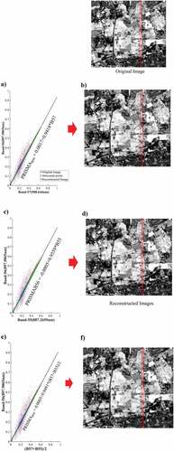
Figure 10. Histograms of the errors (difference observed and the predicted values) for reconstructed image (band 56) based on its consecutive bands. (a) Histogram errors for modeling based on band 57, (b) Histogram errors for modeling based on band 55 and (c) Histogram errors for modeling based on both bands (55, 57).

Results from linear regression modeling of SWIR bands (137; 1736.2556 nm, 143; 1793.6891 nm, 189; 2190.8354 nm, 196; 2245.2136 nm)

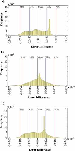
The destriping of the contaminated bands within SWIR bands (137, 189 and 196) showed fairly similar performance to the destriping of contaminated bands in the VNIR spectrum. The robustness of the model can be found in Table 2 and Figures S7(a–f), S8(a–c), S9(a–f), S10(a–c), S11(a–f) and S12(a–c), respectively. However, modeling of abnormal pixels in band 143 showed different results than the other bands. Since multiple adjacent bands are located in the atmospheric water vapor absorption regions (see Table S1), excluded from the analysis, band 165 (1993.2886 nm) was used as the immediate right band to predict and model abnormal pixel values in this band. Regression modeling based on the right band (band 165) showed that band-165 was not highly spectrally correlated with band 143 because the model could not fit a statistically significant relationship between the two bands (Figure 11a,c,e). Therefore, the model with only R band showed the minimum performance with the highest rRMSE (0.5713), highest RMSE (0.0461), lowest R²(0.6126), left-tailed skewness (−0.2603) and high error values range (Table 2 and Figures 11a,c,e and 12 a-c). The visual inspection of the images in the sample sections (Figure 11b) highlighted the algorithm’s low performance in predicting and reconstructing the abnormal pixel values. On the other hand, the destriping based on the immediate left band (142; 1784.4419 nm), with higher spectral similarities, yielded better results qualitatively (Figure 11d) and quantitatively (Figure 11c, and Table 2), minimizing the effect of abnormal pixel values in the entire image. Clearly, the utilization of both bands (bands 165 and 142) suffers the unreliable reconstruction by R band (Table 2 and Figure 12).

Figure 11. Results of abnormal pixel value prediction using spectral-based linear regression in band 143 and neighboring bands. (a) Destriping based on right band (band 165); (b) Reconstructed band based on band 165; (c) Destriping based on left band (band 142); (d) Reconstructed band based on band 142; (e) Destriping based on both bands (bands 138, 136); and (f) Reconstructed band based on both bands (bands 142, 165).

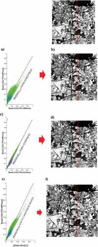
Figure 12. Histograms of the errors (difference observed and the predicted values) for reconstructed image (band 143) based on its consecutive bands. (a) Histogram errors for modeling based on band 165, (b) Histogram errors for modeling based on band 142 and (c) Histogram errors for modeling based on both bands (142, 165).

Discussion

Because the configuration of hyperspectral image collection is somehow similar to traditional push-broom scanners (Pande-Chhetri & Abd-Elrahman, 2011), stripe noises may also occur in hyperspectral sensors, including PRISMA sensor, due to various reasons including sensor calibration (differences), electronic and optic facilities within the sensor, different sensitivities, spectral response variation in the charge-coupled device (CCD), poor sensor radiometric calibration, etc. (Algazi & Ford, 1981; Behroozi et al., 2022; Gadallah et al., 2000; Goodenough et al., 2003; Kang et al., 2015; Lastri et al., 2015; B. Li et al., 2022; Pande-Chhetri & Abd-Elrahman, 2011; Tripathi & Garg, 2020). The stripe noises limit the application of hyperspectral datasets and may cause an error in spectral and spatial base image classification, feature extraction, etc. Despite the noise limitations, PRISMA images are still widely used in various applications (nitrogen content mapping, mineral exploration, ecology, atmospheric studies, etc.) due to their broad-spectrum coverage (Guarini et al., 2017; Travaglini et al., 2007; Vangi et al., 2021). Hence, the striped noise removal in EO satellite imagery, especially hyperspectral sensors, is necessary to obtain homogeneous images and prevent data loss in the imageries.

Among various methods proposed for destriping EO datasets, regression-based techniques (linear, multiple and iterative) are straightforward and robust tools with higher performance than the other models for estimating the variable dataset with a high correlation (Abdul Jabar et al., 2016; Jiang et al., 2009). Given the importance of the PRISMA hyperspectral image in various applications, we implemented spectral-based linear regression to predict pixel abnormalities and image reconstruction in different bands of the PRISMA dataset. The spectral-based linear regression uses highly correlated consecutive bands to predict and reconstruct abnormal pixel values (stripe noises) in the noisy bands. The presence of hundreds of narrow bands in hyperspectral sensors with high spectral correlation (Behroozi et al., 2022; Goetz, 1992) can be a great advantage for predicting abnormal pixel values using the spectral behavior of neighboring bands.

This study showed that the spectral-adjacency-based regression performs accurately in all contaminated bands with stripe noises ranging from VNIR to SWIR spectrum. The performance criteria and visual inspection confirmed the reliable results, except in the two cases discussed in the Results section. Using a combination of two consecutive bands was found to be a better approach for predicting and reconstructing abnormal pixel values with higher accuracy (lower RMSE, higher R² and lower skewness), except when the left or the right band provides large errors. This indicates that the model benefits from the spectral signatures from both bands (left and right bands) to learn, predict and reconstruct the abnormal pixel values, reducing bias between the two bands due to wavelengths differences and better preserving the original image characteristics. Obviously, the lowest model performance was detected when the spectral correlation between the two bands was statistically insignificant (e.g. case of bands 143 and 165).

Therefore, the model is highly dependent on the spectral correlation between consecutive bands: before the model implementation and image reconstruction process, the spectral similarities (spectral correlation) analysis between multiple adjacent bands is a fundamental step.

This confirms our assumption that the algorithm in most cases, where the noisy band (i.e. with abnormal pixel values) and its adjacent bands are not in the atmospheric absorption spectral regions, or the pixel’ spectral reflectance does not abruptly change in the selected bands due to the intrinsic spectral signature, significantly benefits from the spectral similarities (spectral correlation) of both adjacent bands and makes better use of them to predict and reconstruct abnormal pixel values in a straightforward way.

This is an important advantage of this method over other methods that rely on spatial pixel similarities in a single band or multi-source data (auxiliary data, Landsat SLC-on data, etc.) that often may not be available to the target scene (J. Chen et al., 2011; Maxwell et al., 2007). In addition, using spatial-spectral-based pixel similarities may also lead to image inconsistency at the edge pixels because the adjacent pixels may have different inherent characteristics (another surface object, different class, etc.) from the target pixels, leading to model complexity with high computational cost (Y. Chen et al., 2018). Besides, the statistical evaluation specified that the proposed method achieved high accuracy in predicting and reconstructing most of the noisy bands (with stripe noises) in all statistical inferences $\left(rRMSE,RMSE,R^2,\widetilde{m_3}\right)$, in agreement with the accuracies reported in previous published destriping algorithms (Brooks et al., 2018; J. Chen et al., 2011; Maxwell et al., 2007).

Although several algorithms such as machine learning (ML), deep learning (DL) and convolutional neural network (CNN) have been used for destriping of stripe noises in different datasets, the main advantage of our algorithm can easily deal with a dataset containing stripe noises where pixel values change abruptly (non-zero pixel values and non-binary pixel value) and without homogeneity with the adjacent textures. Overall, the proposed algorithm can effectively predict and reconstruct the abnormal pixel values with less computational load and high prediction accuracy. For instance, model performance of our algorithm has comparable results to the findings (B. Li et al., 2022; Deshpande et al., 2021) that used DL methods for destriping of stripe noises, the latter dealing with simulated stripe noises using binary criteria with a higher level of complexity and a higher computational load compared to our method.

Compared with other regression methods, such as quadratic regression methods implemented by Pal et al. (2020) that are mainly based on spatially neighbouring pixels and neighbouring columns, leading to inconsistencies due to different surface objects, different surface texture and surface inhomogeneity, our method uses spectral similarities between adjacent bands (not adjacent pixels), which effectively predict abnormal pixel values with higher accuracy by exploiting the spectral signatures of surface objects. Therefore, our proposed method can be an efficient, straightforward and accurate alternative model for destriping different EO satellite imageries, especially various hyperspectral sensors, due to the high spectral correlation among multiple bands.

The main limitation of the proposed methodology can be attributed to the existence of adjacent consecutive bands located in the atmospheric absorption regions or with a high number of pixels contaminated with noises from different sources, e.g. cloud contaminations, observational geometry inconsistencies, etc., which needs to be removed from the analysis and eventually reduces the spectral similarities between consecutive bands and limits the model implementation.

Nevertheless, it is also possible to predict and reconstruct abnormal pixel values using more adjacent bands that are highly spectrally correlated from first-order or higher-order polynomial functions.

Furthermore, since the spectral-based algorithm is highly dependent on the spectral similarities between adjacent bands, the presence of abrupt changes in pixel’ spectral reflectance in the noisy band and its adjacent bands hinders the model effectiveness. For instance, in the case of band 61 (942.9579 nm; see Figure S3), the correlation between the noisy band and its adjacent bands (bands 60; 939.8600 nm, 62; 951.0114 nm) was statistically low with band 60 due to the proximity of the water vapor absorption around 940 nm (Pu, 2017; Gao et al., 2009; see Table S1).

Conclusion

This research presents a spectral-based regression algorithm to reduce and minimize the effect of stripe noises and abnormal pixel values in PRISMA hyperspectral image. The algorithm was performed on different noisy bands in the PRISMA dataset varying from VNIR to SWIR spectrum, including bands 13, 21, 56, 61, 66, 137, 143, 18 and 196. The visual inspection of the reconstructed bands pointed to the model’s highly acceptable performance in all bands, confirming the homogeneity and continuity of pixels in the pixel abnormality locations. The statistical evaluation referred to the high prediction capability of the model using adjacent bands (left, right or both) in most bands (with a slight difference). In addition, the model exhibited better performance when both bands (right and left) were used in the modeling. Therefore, combining both consecutive bands was highlighted as a better approach for the destriping of PRISMA dataset as the algorithm utilizes the spectral properties of both neighboring bands and minimizes the bias between bands (wavelength differences); thus, it can predict the abnormal pixel values more accurately and better reconstruct the noisy band while preserving the original image characteristics. In contrast, the model showed poor performance when the spectral similarities between two bands were minimum (143; 1793.6891 nm and band 165; 1993.2886 nm) and the wavelength differences between two bands were very high.

The main advantage of the proposed method usable for various hyperspectral sensors is the good accuracy and the lower computational load. In addition, this predicts and reconstructs the stripe noises with highly fluctuating pixel values (non-zero values), abnormal pixel values, based on the spectral relationship between pixels from the noisy band and the corresponded pixels (non-noisy pixels in the same area) in the neighboring bands, i.e. left and right bands or a combination of both; hence, the reconstructed images are more consistent and homogeneous in the abnormal pixel values’ locations compared to the other destriping methods.

On the other hand, the main limitation of this study is the dependency of the algorithm on the spectral similarities between adjacent bands, so that the presence of several consecutive atmospheric absorption bands, or abrupt changes in surface reflectance of land surfaces in the transition from VIS to NIR spectrum, may reduce the spectral similarities with the adjacent bands and, eventually, hinder the modeling of abnormal pixel values. Nevertheless, predicting and reconstructing abnormal pixel values using higher numbers of adjacent bands highly spectrally correlated from first-order or higher-order polynomial functions is also possible.

In addition, the effect of atmospheric absorption gases such as O₃, CO₂ and CH₄ on surface reflectance in different land-cover classes may be considered while dealing with hyperspectral dataset over the urban areas.

The analysis indicated that alongside other multisource and single-source destriping methods, our algorithm could be a reliable, straightforward and highly accurate alternative model for destriping different EO satellite imageries, especially various hyperspectral sensors.

Finally, the experimental comparison of the proposed spectral-adjacency-based algorithm with other models is highly recommended to compare the model efficiency and computational time loads with other models, especially in terms of big data analysis.

Disclosure statement

No potential conflict of interest was reported by the authors.

Data availability statement

Data generated from destriping of PRISMA are mainly provided in the form of tables and figures in the content of manuscript documents. Furthermore, the destriping algorithm data and codes are available upon request from the corresponding author. Additionally, The PRISMA dataset is available from the PRISMA portal (https://prisma.asi.it) (accessed on 20 July 2021).

Supplementary material

Supplemental data for this article can be accessed online at https://doi.org/10.1080/22797254.2022.2141659

Additional information

Funding

This project was financially supported by OPERANDUM, The European Union’s Horizon 2020 Project under grant agreement No.776848.

References

- Abdul Jabar, A., Sulong, G., George, L., Shafry, M., & Abduljabar, Z. (2016). Reconstruction the missing pixels for landsat ETM+SLC-off images using multiple linear regression model. ARO-The Scientific Journal of Koya University, 4(2), 15–24. https://doi.org/10.14500/aro.10147
- Acito, N., Diani, M., & Corsini, G. (2011). Subspace-based striping noise reduction in hyperspectral images. IEEE Transactions on Geoscience and Remote Sensing, 49(4), 1325–1342. https://doi.org/10.1109/TGRS.2010.2081370
- Addink, E. A., & Stein, A. (1999). A comparison of conventional and geostatistical methods to replace clouded pixels in NOAA-AVHRR images. International Journal of Remote Sensing, 20(5), 961–977. https://doi.org/10.1080/014311699213028
- Alevizos, E., Le Bas, T., & Alexakis, D. D. (2022). Assessment of PRISMA level-2 hyperspectral imagery for large scale satellite-derived bathymetry retrieval. Marine Geodesy, 45 (3), 1–23. https://doi.org/10.1080/01490419.2022.2032497
- Algazi, V. R., & Ford, G. E. (1981). Radiometric equalization of nonperiodic striping in satellite data. Computer Graphics and Image Processing, 16(3), 287–295. https://doi.org/10.1016/0146-664X(81)90041-1
- Bartels, M., Wei, H., & Mason, D. C. (2006). DTM generation from LIDAR data using skewness balancing. Proceedings - International Conference on Pattern Recognition, 1, 566–569. https://doi.org/10.1109/ICPR.2006.463
- Behroozi, Y., Yazdi, M., & Asli, A. Z. (2022). Hyperspectral image denoising based on superpixel segmentation low-rank matrix approximation and total variation. Circuits, Systems, and Signal Processing, 41(6), 3372–3396. https://doi.org/10.1007/s00034-021-01938-9
- Bohn, N., Di Mauro, B., Colombo, R., Thompson, D. R., Susiluoto, J., Carmon, N., Turmon, M. J., & Guanter, L. (2022). Glacier ice surface properties in South‐West Greenland Ice Sheet: First estimates from PRISMA imaging spectroscopy data. Journal of Geophysical Research: Biogeosciences, 127(3), 1–21. https://doi.org/10.1029/2021jg006718
- Boloorani, A. D., Erasmi, S., & Kappas, M. (2008). Multi-source remotely sensed data combination: Projection transformation gap-fill procedure. Sensors, 8(7), 4429–4440. https://doi.org/10.3390/s8074429
- Brooks, E. B., Wynne, R. H., & Thomas, V. A. (2018). Using window regression to gap-fill Landsat ETM+ post SLC-Off data. Remote Sensing, 10(10), 1502. https://doi.org/10.3390/rs10101502
- Busetto, L., & Ranghetti, L. (2020). Prismaread: A tool for facilitating access and analysis of PRISMA L1/L2 hyperspectral imagery v1. 0.0. https://doi.org/10.3390/rs10101502
- Chen, Y., Huang, T. Z., & Zhao, X. L. (2018). Destriping of multispectral remote sensing image using low-rank tensor decomposition. IEEE Journal of Selected Topics in Applied earth Observations and Remote Sensing, 11(12), 4950–4967. https://doi.org/10.1109/JSTARS.2018.2877722
- Chen, J., Zhu, X., Vogelmann, J. E., Gao, F., & Jin, S. (2011). A simple and effective method for filling gaps in Landsat ETM+ SLC-off images. Remote Sensing of Environment, 115(4), 1053–1064. https://doi.org/10.1016/j.rse.2010.12.010
- Coppo, B., Faraci, S., & Cosi. (2019). Leonardo spaceborne infrared payloads for earth observation: SLSTRs for copernicus sentinel 3 and PRISMA hyperspectral camera for PRISMA satellite. Proceedings, 27(1), 1. https://doi.org/10.3390/proceedings2019027001
- Darvishi Boloorani, A., Erasmi, S., & Kappas, M. (2008). Multi-source image reconstruction: Exploitation of EO-1/ALI in Landsat-7/ETM+ SLC-off gap filling. Image Processing: Algorithms and Systems VI, 6812, 681219. https://doi.org/10.1117/12.766866
- David, F. N. (1953). A statistical primer. A Statistical Primer.
- Davies, O. L. (1947). Statistical methods in research and production. Statistical Methods in Research and Production, 3rd ed., New York: Hafner Press.
- Deshpande, A. M., Patale, S. R., & Roy, S. (2021). Removal of line striping and shot noise from remote sensing imagery using a deep neural network with post-processing for improved restoration quality. International Journal of Remote Sensing, 42(19), 7357–7380. https://doi.org/10.1080/01431161.2021.1957512
- Farooq, S. (2010). Hyperspectral remote sensing. Current Science, 98(6).
- Folks, J. L., & Chhikara, R. S. (1978). The inverse Gaussian distribution and its statistical application—A review. Journal of the Royal Statistical Society: Series B (Methodological), 40(3), 263–275. https://doi.org/10.1111/j.25176161.1978.tb01039.x
- Gadallah, F. L., Csillag, F., & Smith, E. J. M. (2000). Destriping multisensor imagery with moment matching. International Journal of Remote Sensing, 21(12), 2505–2511. https://doi.org/10.1080/01431160050030592
- Gao, B. C., Montes, M. J., Davis, C. O., & Goetz, A. F. H. (2009). Atmospheric correction algorithms for hyperspectral remote sensing data of land and ocean. Remote Sensing of Environment, 113(SUPPL. 1), S17–S24. https://doi.org/10.1016/j.rse.2007.12.015
- Goetz, A. F. H. (1992). Imaging spectrometry for Earth remote sensing. International Union of Geological Sciences, 15(1), 7–14. https://doi.org/10.18814/epiiugs/1992/v15i1/003
- Goodenough, D. G., Dyk, A., Niemann, K. O., Pearlman, J. S., Chen, H., Han, T., Murdoch, M., & West, C. (2003). Processing Hyperion and ALI for forest classification. IEEE Transactions on Geoscience and Remote Sensing, 41(6 PART I), 1321–1331. https://doi.org/10.1109/TGRS.2003.813214
- Guarini, R., Loizzo, R., Longo, F., Mari, S., Scopa, T., & Varacalli, G. (2017). Overview of the PRISMA space and ground segment and its hyperspectral products. 2017 IEEE International Geoscience and Remote Sensing Symposium (IGARSS), 431–434.
- Guo, Y., Chen, J., Wang, J., Chen, Q., Cao, J., Deng, Z., Xu, Y., & Tan, M. (2020). Closed-loop matters: Dual regression networks for single image super-resolution. Proceedings of the IEEE Computer Society Conference on Computer Vision and Pattern Recognition, 5406–5415. https://doi.org/10.1109/CVPR42600.2020.00545
- Han, T., Goodenough, D. G., Dyk, A., & Love, J. (2002). Detection and correction of abnormal pixels in Hyperion images. International Geoscience and Remote Sensing Symposium (IGARSS), 3(C), 1327–1330. https://doi.org/10.1109/igarss.2002.1026105
- Jiang, Y., Lan, T., & Wu, L. (2009). A comparison study of missing value processing methods in time series data mining. 2009 International Conference on Computational Intelligence and Software Engineering, 1–4. https://doi.org/10.1109/CISE.2009.5365076
- Kang, W., Yu, S., Seo, D., Jeong, J., & Paik, J. (2015). Push-broom-type very high-resolution satellite sensor data correction using combined wavelet-Fourier and multiscale non-local means filtering. Sensors (Switzerland), 15(9), 22826–22853. https://doi.org/10.3390/s150922826
- Lastri, C., Guzzi, D., Barducci, A., Pippi, I., Nardino, V., & Raimondi, V. (2015). Striping noise mitigation: Performance evaluation on real and simulated hyperspectral images. Image and Signal Processing for Remote Sensing XXI, 9643, 96430K. https://doi.org/10.1117/12.2195706
- Licciardi, G., & Chanussot, J. (2018). Spectral transformation based on nonlinear principal component analysis for dimensionality reduction of hyperspectral images. European Journal of Remote Sensing, 51(1), 375–390. https://doi.org/10.1080/22797254.2018.1441670
- Li, Q., Zhong, R., & Wang, Y. (2019). A method for the destriping of an orbita hyperspectral image with adaptive moment matching and unidirectional total variation. Remote Sensing, 11(18). https://doi.org/10.3390/rs11182098
- Li, B., Zhou, Y., Xie, D., Zheng, L., Wu, Y., Yue, J., & Jiang, S. (2022). Stripe noise detection of high-resolution remote sensing images using deep learning method. Remote Sensing, 14(4). https://doi.org/10.3390/rs14040873
- Loizzo, R., Daraio, M., Guarini, R., Longo, F., Lorusso, R., DIni, L., & Lopinto, E. (2019). PRISMA mission status and perspective. International Geoscience and Remote Sensing Symposium (IGARSS), 4503–4506. https://doi.org/10.1109/IGARSS.2019.8899272
- Ma, Q., Jiang, J., Liu, X., & Ma, J. (2022). Deep unfolding network for spatiospectral image super-resolution. IEEE Transactions on Computational Imaging, 8(1), 28–40. https://doi.org/10.1109/TCI.2021.3136759
- Matheron, G. (1963). Principles of geostatistics. Economic Geology, 58(8), 1246–1266. https://doi.org/10.2113/gsecongeo.58.8.1246
- Maxwell, S. K., Schmidt, G. L., & Storey, J. C. (2007). A multi-scale segmentation approach to filling gaps in Landsat ETM+ SLC-off images. International Journal of Remote Sensing, 28(23), 5339–5356. https://doi.org/10.1080/01431160601034902
- Pal, M. K., Porwal, A., & Rasmussen, T. M. (2020). Noise reduction and destriping using local spatial statistics and quadratic regression from Hyperion images. Journal of Applied Remote Sensing, 14(1), 1. https://doi.org/10.1117/1.jrs.14.016515
- Pande-Chhetri, R., & Abd-Elrahman, A. (2011). De-striping hyperspectral imagery using wavelet transform and adaptive frequency domain filtering. ISPRS Journal of Photogrammetry and Remote Sensing, 66(5), 620–636. https://doi.org/10.1016/j.isprsjprs.2011.04.003
- Pringle, M. J., Schmidt, M., & Muir, J. S. (2009). Geostatistical interpolation of SLC-off Landsat ETM+ images. ISPRS Journal of Photogrammetry and Remote Sensing, 64(6), 654–664. https://doi.org/10.1016/j.isprsjprs.2009.06.001
- Pu, R. (2017). Hyperspectral Remote Sensing: Fundamentals and Practices (1st ed.). CRC Press. https://doi.org/10.1201/9781315120607
- Qu, Y., Zhang, X., Wang, Q., & Li, C. (2018). Extremely sparse stripe noise removal from nonremote-sensing images by straight line detection and neighborhood grayscale weighted replacement. IEEE Access, 6, 76924–76934. https://doi.org/10.1109/ACCESS.2018.2883459
- Rakwatin, P., Takeuchi, W., & Yasuoka, Y. (2007). Stripe noise reduction in MODIS data by combining histogram matching with facet filter. IEEE Transactions on Geoscience and Remote Sensing, 45(6), 1844–1855. https://doi.org/10.1109/TGRS.2007.895841
- Roy, D. P., Ju, J., Lewis, P., Schaaf, C., Gao, F., Hansen, M., & Lindquist, E. (2008). Multi-temporal MODIS–Landsat data fusion for relative radiometric normalization, gap filling, and prediction of Landsat data. Remote Sensing of Environment, 112(6), 3112–3130. https://doi.org/10.1016/j.rse.2008.03.009
- Scaramuzza, P., Micijevic, E., & Chander, G. (2004). SLC gap-filled products: Phase one methodology. 1–5. https://landsat.usgs.gov/documents/SLC_Gap_Fill_Methodology.pdf.
- Seydi, S. T., & Hasanlou, M. (2017). A new land-cover match-based change detection for hyperspectral imagery. European Journal of Remote Sensing, 50(1), 517–533. https://doi.org/10.1080/22797254.2017.1367963
- Sun, Y. J., Huang, T. Z., Ma, T. H., & Chen, Y. (2019). Remote sensing image stripe detecting and destriping using the joint sparsity constraint with iterative support detection. Remote Sensing, 11(6), 608. https://doi.org/10.3390/rs11060608
- Tang, X., Dong, S., Luo, K., Guo, J., Li, L., & Sun, B. (2022). Noise removal and feature extraction in airborne radar sounding data of ice sheets. Remote Sensing, 14(2), 1–16. https://doi.org/10.3390/rs14020399
- Travaglini, D., Barbati, A., Chirici, G., Lombardi, F., Marchetti, M., & Corona, P. (2007). ForestBIOTA data on deadwood monitoring in Europe. Plant Biosystems - An International Journal Dealing with All Aspects of Plant Biology, 141(2), 222–230. https://doi.org/10.1080/11263500701401778
- Tripathi, P., & Garg, R. D. (2020). First impressions from the PRISMA hyperspectral mission. Current Science, 119(8), 1267–1281. https://doi.org/10.18520/cs/v119/i8/1267-1281
- van der Meer, F. (2012). Remote-sensing image analysis and geostatistics. International Journal of Remote Sensing, 33(18), 5644–5676. https://doi.org/10.1080/01431161.2012.666363
- Vangi, E., D’amico, G., Francini, S., Giannetti, F., Lasserre, B., Marchetti, M., & Chirici, G. (2021). The new hyperspectral satellite PRISMA: Imagery for forest types discrimination. Sensors (Switzerland), 21(4), 1–19. https://doi.org/10.3390/s21041182
- Verrelst, J., Rivera-Caicedo, J. P., Reyes-Muñoz, P., Morata, M., Amin, E., Tagliabue, G., Panigada, C., Hank, T., & Berger, K. (2021). Mapping landscape canopy nitrogen content from space using PRISMA data. ISPRS Journal of Photogrammetry and Remote Sensing, 178(June), 382–395. https://doi.org/10.1016/j.isprsjprs.2021.06.017
- Wang, B., Bao, J., Wang, S., Wang, H., & Sheng, Q. (2017). Improved line tracing methods for removal of bad streaks noise in CCD line array image—A case study with GF-1 images. Sensors (Switzerland), 17(4), 1–10. https://doi.org/10.3390/s17040935
- Wang, B., Zou, Y., Zhang, L., Li, Y., Chen, Q., & Zuo, C. (2022). Multimodal super-resolution reconstruction of infrared and visible images via deep learning. Optics and Lasers in Engineering, 156, 107078 . https://doi.org/10.1016/j.optlaseng.2022.107078
- Wijedasa, L. S., Sloan, S., Michelakis, D. G., & Clements, G. R. (2012). Overcoming limitations with Landsat imagery for mapping of peat swamp forests in Sundaland. Remote Sensing, 4(9), 2595–2618. https://doi.org/10.3390/rs4092595
- Yin, G., Mariethoz, G., & McCabe, M. F. (2017). Gap-filling of landsat 7 imagery using the direct sampling method. Remote Sensing, 9(1), 1–20. https://doi.org/10.3390/rs9010012
- Yin, G., Mariethoz, G., Sun, Y., & McCabe, M. F. (2017). A comparison of gap-filling approaches for landsat-7 satellite data. International Journal of Remote Sensing, 38(23), 6653–6679. https://doi.org/10.1080/01431161.2017.1363432
- Zeng, C., Shen, H., & Zhang, L. (2013). Recovering missing pixels for Landsat ETM+ SLC-off imagery using multi-temporal regression analysis and a regularization method. Remote Sensing of Environment, 131, 182–194. https://doi.org/10.1016/j.rse.2012.12.012
- Zhang, K., Gool, L. V., & Timofte, R. (2020). Deep unfolding network for image super-resolution. Proceedings of the IEEE/CVF Conference on Computer Vision and Pattern Recognition, 3217–3226.
- Zhang, C., Li, W., & Travis, D. (2007). Gaps-fill of SLC-off Landsat ETM+ satellite image using a geostatistical approach. International Journal of Remote Sensing, 28(22), 5103–5122. https://doi.org/10.1080/01431160701250416