Freight train air brake models

ABSTRACT

This paper is an outcome of an international collaborative research initiative. Researchers from 24 institutions across 12 countries were invited to discuss the state-of-the-art in railway train air brake modelling with an emphasis on freight trains. Discussed models are classified as empirical, fluid dynamics and fluid-empirical dynamics models. Empirical models are widely used, and advanced versions have been used for train dynamics simulations. Fluid dynamics models are better models to study brake system behaviour but are more complex and slower in computation. Fluid-empirical dynamics models combine fluid dynamics brake pipe models and empirical brake valve models. They are a balance of model fidelity and computational speeds. Depending on research objectives, detailed models of brake rigging, friction blocks and wheel-rail adhesion are also available. To spark new ideas and more research in this field, the challenges and research gaps in air brake modelling are discussed.

KEYWORDS:

• Air brake
• freight railway
• empirical models
• fluid dynamics
• train dynamics
• brake valves
• brake pipes
• adhesion

1. Introduction

The air brake is one of the most important systems in railway trains. Freight trains, to some extent, pose greater challenges for air brakes than shorter passenger trains do, in the sense that freight trains are significantly longer and heavier. The issue of brake delays, one of the most interesting issues about air brakes, is also more evident in freight trains. This paper focuses on dynamics models that can be used for freight train air brake simulations. References related to passenger trains were also reviewed as their modelling methods can also be used for freight train air brake modelling. Air brakes are the most common type of brakes in railway operations; non-mainstream brake systems such as aerodynamic, eddy current and electromagnetic brakes are not discussed in this paper. Dynamic braking that uses traction motors as a part of the brake system is also out of the scope. This paper focuses on modern air brakes. Straight air brakes and vacuum brakes cannot meet the requirements of modern freight transport and are therefore not discussed in this paper either.

A simplified illustration of typical air brake systems is shown in Figure 1. Note that air brake systems can vary significantly in different countries and regions, and this figure does not cover all variations. However, most modern air brake systems are derived from the well-known Westinghouse triple valve. Variations shown in the figure include the emergency reservoir for typical systems that follow Association of American Railroads (AAR) standards and a command reservoir for typical systems that follow International Union of Railways (UIC) standards. On some Australian (AUS) and Chinese (CHN) systems, an accelerated release reservoir is also used. Other than these, relayed systems that have a supplementary reservoir and a relay valve are also being using in Australia. These relayed variations can be based on AAR standard brake systems or Australian versions of brake systems. Twin pipe systems that have a second brake pipe running along the train have been reported from Europe and India. The second pipe is used as an air supply pipe to directly feed the auxiliary reservoir upon brake release. This removes the air consumption from the main pipe and can therefore be seen as a feature for accelerated release, as the main pipe pressure will rise significantly quicker in long trains.

Figure 1. Typical freight train air brake systems.

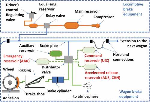
Traditionally, brake and release signals to individual wagons are transmitted via pressure changes in brake pipes. Due to the physical limits of air wave propagations, brake and release signals in traditional brake systems have an evident delay from the signal sources to remote wagons. To minimize the signal delays, the innovation of Electronically Controlled Pneumatic (ECP) brake systems [1] was developed. In ECP systems, an electrical signal cable was fitted along with the brake pipe. The electrical cable can directly send brake and release signals to distributor valves on individual wagons so as to eliminate the delays caused by brake pipe pressure changes. The brake pipe in this case serves the purpose of air supply to individual wagons without being the brake and release signal media. From the dynamics modelling perspective, modelling of ECP brakes can be regarded as easier than that of traditional air brake systems. This is mainly because the electronic parts of ECP brakes are often not included or are simplified in dynamics modelling; and ECP brakes have more consistent braking behaviour among individual wagons, therefore removing one more variation for the modelling process.

Air brake models are important and can be used for numerous applications. The most widely seen application is to calculate train-braking distance, which can be further used to approve new equipment (brake valves, brake shoes, etc.), track slopes/gradients, and train configurations. Braking distance is also a critical piece of information in the design process of railway signalling and automatic train driving. Air brake models have also been regarded as one of the most important components in Longitudinal Train Dynamics (LTD) simulations as braking usually generates large in-train forces. In-train forces are one of the focuses of LTD studies, which are also often reviewed during the previously mentioned approvals for equipment, etc. Another motivation for brake studies is that brake applications usually generate large compressive in-train forces which, from vehicle dynamics perspectives, pose higher risks than tensile forces on curves. In addition to these purposes, brake models are required in train driving simulators to provide realistic driver training scenarios. Real-time train dynamics simulations, which require much faster air brake simulations, are also required for driver advisory systems and Automatic Train Operations.

Air brake simulations are challenging due to their nonlinear fluid dynamic nature, complex valve devices and the limits from parameter determination or identification. The strong nonlinearities require computationally expensive solving techniques such as the Finite Element Method (FEA) and Method of Characteristics (MoC). In addition, numerous valves are used in air brake systems; these valves usually have high complexity and are very sensitive to model parameter variations. One of the most challenging issues about air brake modelling is probably the determination of model parameters. Some model parameters, such as brake pipe friction, valve sliding friction, and orifice friction, also have strong nonlinearities and are practically impossible to measure. More challenges about air brake modelling will be discussed at the end of the paper.

This paper reviews railway air brake modelling methods. Typical features of modern air brake systems (Section 2) are introduced first for a better physical understanding of subsequent brake system discussions and modelling method reviews. Modelling methods are classified into two groups: empirical brake pressure and force models (Section 3), and fluid and fluid-empirical dynamics brake system models (Section 4). The former group directly focus on brake cylinder pressure and brake force behaviours, and hence do not include brake pipe models. The latter group commonly model brake pipe behaviour first by following fluid dynamics principles (Section 4.1), and cylinder pressures and brake forces are then determined using empirical (Section 4.3) or fluid dynamics (Section 4.4) brake valve models. The ones that have used empirical valve models are called fluid-empirical dynamics brake system models. Section 5 reviews common methods used to convert brake cylinder pressures to brake forces and Section 6 reviews the considerations of wheel-rail adhesion in brake models. Section 7 discusses the challenges and research gaps in air brake modelling along with various other brake-related issues. Section 8 presents conclusions. This paper is focussed on enabling readers to better understand the state-of-the-art of air brake modelling and sparking new research on this topic.

2. Typical features of modern air brake systems

As shown in Figure 1, in typical air brake systems, a compressor is fitted on the locomotive to produce compressed air that is then stored in the main reservoir. The driver’s control valve can select the options of charging compressed air from the main reservoir to the brake pipe or discharging the air in the brake pipe to atmosphere. Modern railway air brakes have evolved to have the so-called ‘fail-safe’ feature that basically means that, if the brake pipe has severe leakage or pull-apart, the train will automatically apply the air brake. This fail-safe feature also means that, when the brake pipe is being discharged, the train applies brakes whilst, when the brake pipe is being charged, the train releases the brakes.

On individual wagons, the compressed air is stored in auxiliary reservoirs. As shown in Figure 2, distributor valves determine the connection passages among auxiliary reservoirs, brake pipes, brake cylinders and atmosphere. During brake applications, compressed air flows from auxiliary reservoirs to brake cylinders and then presses the brake shoes against the wheel treads via brake riggings. During brake release, distributor valves let compressed air in brake cylinders discharge to atmosphere so as to release the pressure on brake shoes. Apart from the basic brake and release function, modern railway air brakes have many other features that will be discussed later in this section.

Figure 2. Basic triple valve actions: (a) release, (b) brake and (c) lapping.

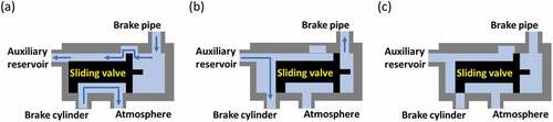
Modern air brake systems were mainly derived from the well-known Westinghouse triple valve. The basic working mechanism of triple valves is shown in Figure 2. The sliding valve is the key component that moves under the pressure differences between auxiliary reservoir and brake pipe. At different positions, sliding valves can form different air passages among brake pipes, auxiliary reservoirs, brake cylinders and atmosphere. In modern air brake systems, more features have been added to the triple valve. For example, an extra valve called a regulating valve is usually embedded in the sliding valve to achieve more switching options and regulation of various air passages. Meanwhile, the term ‘distributor’ or ‘distributor valve’ has been widely used to replace the name of triple valve. Wagon brake equipment has also been integrated with other valves such as the emergency valve, quick-release valve and quick application valve. This section briefly introduces some common features of modern air brake systems. Note that different systems have a different combination of features as shown in Table 1. In this table, ABDX is one of the most common AAR freight brake systems; KE is one of the most common UIC freight brake systems; WF 5 is one of the most common freight brake systems used in Australia (AUS); 102–1 is one of the most common air brake systems used in China (CHN); and KAB60 is a popular brake system used in Russia (RUS).

Table 1. Typical features of modern air brake systems.

Valve type	ABDX [107]	KE [79]	WF 5 [110]	120–1 [94]	KAB60 [115]
Feature	(AAR)	(UIC)	(AUS)	(CHN)	(RUS)
Service brake	YES	YES	YES	YES	YES
Quick action	YES	YES	YES	YES	YES
Quick service	YES	YES	YES	YES	YES
Lapping	YES	YES	YES	YES	YES
Release	YES	YES	YES	YES	YES
Accelerated release	YES	NO	YES	YES	YES
Retarded recharge	YES	YES	YES	YES	YES
Graduated release	NO	YES	NO	NO	YES
Emergency portion	YES	NO	NO	YES	NO

In this paper, different brake scenarios are normally characterized by brake pipe pressure reductions. For example, 50 kPa pressure reduction for minimum service brake, 170 kPa pressure reduction for full-service brake and 600-kPa pressure reduction for emergency air brake. Note that these pressure reductions were calculated from the maximum brake pipe pressure (e.g., 500 kPa or 600 kPa) and can be regarded as the brake commands. With these brake commands, pressurized air can be discharged from the brake pipe via leading locomotives, remote locomotives (for Distributed Power, i.e., DP trains) and End-of-Train devices (if used).

2.1. Service brake

Service brake is a basic feature of any brake system, during which pressurized air flows from auxiliary reservoir to brake cylinder. Brakes can be applied at smaller pressure reductions and then moved to larger pressure reductions, i.e., graduated brakes. To avoid undesired air brakes, brake systems are designed to have a minimum service brake (e.g., 50 kPa pressure reduction), i.e., pipe pressure reduction lower than the minimum pressure reduction will not be responsive. Also brake distributors are designed to properly ignore very slow variations of pipe pressure without penalizing too much speed and precision of valve response. Service brakes are also capped by full-service brake (e.g., 170 kPa pressure reduction) that is the maximum pressure reduction before emergency brakes are triggered.

2.2. Quick action

At the beginning of a brake application, the brake valve forms a passage between the brake pipe and a small internal volume called the quick action bulb (also called an accelerating chamber in some systems) so as to quickly reduce brake pipe pressure. This feature has two functions: (1) to accelerate the brake process in an individual wagon; and (2) to accelerate pressure reductions in the brake pipe so as to decrease brake delays. The usage of quick action bulbs also helps to increase the stability of the brake valves to avoid undesired braking as it takes a reasonable amount of air to fill the quick action bulb and then to trigger subsequent actions; and this amount of air can only result from driver actions or system failures like broken pipes.

2.3. Quick service

After the quick action process, the sliding valve moves to connect auxiliary reservoir and brake cylinder. Before cylinder pressure reaches a certain level (e.g., 60 kPa), the sliding valve allows an extra air passage directly from brake pipe to brake cylinder. This feature has the two functions described in the quick action feature. In addition, the quick service feature also helps to overcome static friction in brake cylinders to extend the push rods and quickly bring the brake shoes into physical contact with the running gear.

2.4. Lapping

When the auxiliary reservoir pressure is balanced by brake cylinder pressure, the regulating valve will move back to block the passage between the auxiliary reservoir and brake cylinder. After this, the pressure differences between these two are small, sliding valves are not moving, brake release is not activated. Therefore, the main function of the lapping feature is to hold the brake pressure at a certain level.

2.5. Release

When brake pipe pressure is higher than auxiliary reservoir pressure, regulating valves and sliding valves move to connect brake cylinders to atmosphere. For air brake systems that do not have the graduated-release function, this release process cannot be paused once started. During the release process, connections from the brake pipe to various reservoirs and chambers (e.g., auxiliary reservoir, quick-release reservoir, and emergency bulb) are also established, therefore pressurized air can be recharged from the brake pipe to these reservoirs and chambers.

2.6. Accelerated release

The accelerated-release feature requires an accelerated-release valve. When brake release is activated, air flow from brake cylinder to atmosphere triggers the quick-release valve to open an air passage from quick-release reservoir (e.g., WF 5 and 210–1 systems) or emergency reservoir (e.g., ABDX) to brake pipe. Similar to the quick action feature, the accelerated release also serves two main functions but now by increasing brake pipe pressure: (1) it accelerates the brake release process of individual wagons; and (2) it increases brake pipe pressures to reduce release action delays in the train.

2.7. Retarded recharge

During the release process, the locomotive main reservoir recharges the brake pipe. When brake pipe pressure is significantly higher than auxiliary reservoir pressure, sliding valves will be over-pushed to decrease the opening size between brake pipe and auxiliary reservoir. This feature regulates auxiliary reservoir recharging rates at different positions of the train to help achieve a uniform release process along the train.

2.8. Graduated release

This feature is commonly seen on European systems where a command reservoir is used and connected to the brake pipe via a cut-off valve. To release the brake, brake pipe needs to be continuously charged to maintain a higher pressure than the command reservoir. Otherwise, brake pipe pressure will be slowly balanced by the command reservoir via the check valve. In other words, brake release can be paused (graduated) by pausing the charging of the brake pipe.

2.9. Emergency portion

Some brake systems (e.g., ABDX and 120–1 systems) have an emergency brake valve that is additional to the main valve for service brake and release. During emergency brake, the emergency valve detects the significant pressure drop in brake pipe and then opens a passage to atmosphere to directly dump pressurized air from the brake pipe. The ABDX system (not used in the 120–1 system) then uses both auxiliary reservoir and emergency reservoir to charge brake cylinders so as to achieve fast and sufficient brakes.

3. Empirical brake pre ssure and force models

Such models directly focus on the behaviours of brake cylinder pressures and/or brake forces applied on wheels; due to this focus, brake pipe models were not directly needed. Empirical models use mathematical equations (not necessarily referring to fluid dynamics principles) to fit the measured characteristics of air brake systems. Five different methods are reviewed in this section: (1) equivalent constant pressures/forces, (2) look-up tables, (3) power functions, (4) natural exponential equations, and (5) polynomial equations.

3.1. Constant force models

Early work in the 1950s by Lazaryan [2], a former Union of Soviet Socialist Republics (USSR) researcher, modelled a freight train as a continuum rod. Due to the lack of computing power, brake forces were modelled as constant forces to allow development of differential equations and manual solutions. Despite the computing power limitations, the model had considered brake delays by applying brake forces from the head to the tail of the rod. Lazaryan later published another interesting article where he used an electrical model to simulate train braking [3]. In this electrical model, voltages were used as brake forces and sequentially applied to different nodes (wagons) of the circuit.

Howard et al. [4] reviewed 27 Train Performance Simulation models that were mainly used to determine train speeds, brake, and traction capabilities of a single train. These authors mentioned that a popular way to simulate train braking then was to ignore the transitions of brake forces during brake applications and release, i.e., assume the brake forces are constant.

With the availability of digital computers, constant brake force models are still being used for applications such as headway design and signalling design. In a signalling design tool developed by Queensland Rail in Australia [5], brake forces were modelled as constants with the consideration of brake delays. The purpose of this tool was to calculate the stopping distance of certain trains. Presciani et al. [6] described a brake model used in an Automatic Train Protection (ATP) system to calculate train braking distance. In this model, the brake force ascending process was regarded as a linear process and modelled as an equivalent step function rather than a ramp function. After this equivalisation, brake forces were then modelled as a constant value for a specific brake scenario. Brosseau et al. [7] developed a braking enforcement algorithm to be used for ATP systems. Empirical formulas were developed to convert different pressure ascending times of different vehicles of the train to a single equivalent pressure ascending time. In this way, the braking enforcement action can be assessed by using only three parameters: initial brake pressure, equivalent ascending time and final brake pressure. This model was later used by Mitsch et al. [8] for the development of a train control algorithm.

Brake forces can also be considered constant when detailed characteristics of the air brake system are not of interest. Reibenschuh et al. [9] and Kuciej et al. [10] studied frictional heat on brake pads during brake applications. In these two studies, brake forces were also modelled as constant forces.

3.2. Look-up tables

The look-up table method is a simple modelling approach that uses array indexing operations, interpolations, and extrapolations; it can significantly simplify the modelling process and has the advantage of having fast computing speed. Air brake modelling using this method can be as simple as a single-dimensional look-up table as used in [11–14]. Brake system characteristics considered in these models were maximum brake pressure (or force) and pressure (or force) ascending time. Brake delays and other details were neglected. Howard et al. [4] reported that look-up table models were also one of the three most popular air brake models used in Train Performance Simulation models in the late 1980s. The other two models were constant force models, which have been reviewed in this paper, and the use of various empirical functions that will be reviewed later. Murtaza and Garg [15] reported a look-up table that was used in Europe in the 1970s. This model used piece-wise-linear look-up tables to model brake cylinder pressures measured from field and laboratory tests.

Martin and Hay [16] used a two-dimensional look-up table to model freight train air brakes, in which brake cylinders pressures were expressed as:

(1) $P_b\left(i,t\right)=\frac{i{P}_{b,1}\left(t\right)+\left(150-i\right)P_{b,150}\left(t\right)}{150}$(1)

where $P_b$ is brake cylinder pressure of the vehicle of interest; $t$ is time; $i$ is the $i^{th}$ vehicle of the train; $P_{b,1}$ is the brake cylinder pressure of the first vehicle of the train; and $P_{b,150}$ is the brake cylinder pressure of the ${150}^{th}$ vehicle of the train. Cylinder pressures of the first and last vehicles of the consist were used as reference pressures. Cylinder pressures in between were then interpolated by indexing the position of the vehicle interest. In the Martin and Hay model, the look-up tables for the references cylinder pressures were developed from measured data. Different reference cylinder pressures were stored in the model for different brake scenarios (e.g., minimum service brake, full-service brake, and emergency brake). The utilization of measured data means that the model, ideally, considers all characteristics of the brake system in the measured braking scenarios. In addition to maximum pressures and pressure ascending time, other details such as fast pressure increases resulting from quick service and cylinder pressure variations resulted from cylinder piston movements can also be considered. The Martin and Hay model also considered brake delays by starting the look-up table process at different times. Two different delays were considered in the model: one for service brake and the other for emergency brake.

An interesting look-up table model was developed by Blokhin et al. [17,18], which was expressed as:

(2) $P_{shoe}\left(t_e\right)={\delta }_{rigging}\sum _{j=1}^n\left[{P_b}_j+\frac{{P_b}_{j+1}-{P_b}_j}{t_{j+1}-t_j}\left(t_e-t_j\right)\right]\mathrm{H}\left(t_e-t_j\right)\mathrm{H}\left(t_{j+1}-t_e\right)$(2)

(3) $t_e=t-t_{delay,system}-t_{delay,valve}$(3)

where $P_{shoe}$ is brake pressure on brake shoes; $t_e$ is the effective time in the brake or release process; $t_{delay,system}$ is the time delay of the brake system; $t_{delay,valve}$ is the delay of the valve action; ${\delta }_{rigging}$ is the rigging factor; $j$ is the sequence of data points in the look-up table; $n$ is the total number of data points; $t_j$ a nd ${P_b}_j$ are the values of the $j^{th}$ data point; and $\mathrm{H}$ is a unit step function. This model directly calculates brake pressures on brake shoes by using a rigging factor. The interesting point is that the model is programming-ready by using the effective time ($t_e$) and the unit step functions ($\mathrm{H}$). $t_e$ and $\mathrm{H}$ make the model active only when time is between $t_j$ and $t_{j+1}$ and the pressure variation process is an accumulative process. A similar approach was used by Pudovikov et al. [19] in the development of algorithms for automatic control of freight trains. Their work used the experimental data published by Nikiforov et al. [20].

Cruceanu [21] summarized experimental data and then used the following equation to model brake cylinder filling characteristics:

(4) $P_b=0.4+\frac{t-4}{t_{max,95\mathrm{\%}}}{P}_{b,max}\approx \left(0.1+\frac{t-4}{t_{max,95\mathrm{\%}}}\right)P_{b,max}$(4)

where $t_{max,95\mathrm{\%}}$ is the time needed to reach 95% of maximum brake cylinder pressure and $P_{b,max}$ is the maximum brake cylinder pressure.

A look-up table air brake model was included in the commercial software package called Universal Mechanism [22]. The air brake model is similar to the one developed by Martin and Hay [16]. The UM air brake model considers different brake delays for service brake, emergency brake and brake release. It also allows the utilization of many reference brake cylinder pressures and a brake malfunction mode. When the brake equipment of a specific vehicle is in working order, its cylinder pressure is linearly interpolated from the two nearest reference pressures. When the brake equipment malfunctions, the cylinder pressure was set to be zero. Lingaitis et al. [23] used a two-dimensional (time and vehicle index) look-up table to determine brake cylinder pressures while Pshinko et al. [24] used the same method to determine brake shoe normal forces.

3.3. Power function

In an early publication, Grebenyuk [25] reviewed a number of in-train force assessment models that have considered the implications of air brake applications. In these models, air brakes were approximated and integrated into in-train force models. In other words, these models directly delivered in-train forces rather than brake cylinder pressures or brake forces. According to Grebenyuk, the first model as such was published by an American researcher Winkander in [26]. This quite early model was very empirical and simply expressed as the concept that the maximum in-train forces during brake application equals half of the total brake forces of the train. Subsequently, a USSR researcher Karvatchi [27] developed a new model by analysing the train as a linear mass-spring system:

(5) $F_{c,max}=\frac{1}{8}n{F}_{b,max}\frac{t}{t_{max}}$(5)

where $F_{c,max}$ is the maximum coupler force of the train; $n$ is the total number of vehicles in the train; $F_{b,max}$ is the maximum brake force of an individual vehicle; $t_{max}$ is the time needed for brake forces to reach their maximum steady values, i.e., the pressure ascending time. It can be seen that Karvatchi’s model shares a similar rationale to Wikander’s model but has smaller approximated in-train forces (from 1/2 to 1/8) and a time varying process. Equation (5)(5) $F_{c,max}=\frac{1}{8}n{F}_{b,max}\frac{t}{t_{max}}$(5) also indicates that air brake force variations were regarded as a linear process. Later, Grebenyuk [25] further developed the Karvatchi formula by analysing experimental results to produce:

(6) $F_{c,max}=K_a\frac{\left(1-{0.5}^{\delta }\right)}{2\left(\delta +1\right)}{F}_{b,max}{\left(\frac{t}{t_{max}}\right)}^{\delta }$(6)

where $K_a$ is a parameter to differentiate maximum tensile forces and compressive forces; $\delta$ is a system characterizing parameter that needs to be tuned for specific types of air brake systems. Equation (6)(6) $F_{c,max}=K_a\frac{\left(1-{0.5}^{\delta }\right)}{2\left(\delta +1\right)}{F}_{b,max}{\left(\frac{t}{t_{max}}\right)}^{\delta }$(6) kept the brake force variation part ($t$ and $t_c$) but in a power function form. Reaching this stage, Grebenyuk’s model has thus been improved to be a nonlinear model. More parameters have been added ($K_a$ and $\delta$) to allow better fittings of various types of brake systems.

In another later work by Grebenyuk [28], air brae models were separated from in-train force models. These air brake models were expressed as:

(7) $P_b\left(t,x_L\right)=\left\{\begin{array}{cc}0& t\le \frac{x_L}{L}{t}_{delay,max}\\ P_{b,max}\frac{{\left(t-\frac{x_L}{L}{t}_{delay,max}\right)}^{\delta }}{t_{asending}}& \frac{x_L}{L}{t}_{delay,max}<t<\frac{x_L}{L}{t}_{delay,max}+t_{asending}\\ P_{b,max}& \frac{x_L}{L}{t}_{delay,max}+t_{asending}\le t\end{array}\right.$(7)

where $x_L$ is distance of the vehicle from the signal source locomotive; $L$ is the total length of the train or string of vehicles; $t_{delay,max}$ is the brake delay of the last vehicle of the train; $P_{b,max}$ is the maximum brake cylinder pressure; and $t_{asending}$ is the cylinder pressure ascending time. The model can be used to simulate different types of air brake system by adjusting the system characteristics parameter $\delta$. Cylinder pressure ascending time $t_2$ can also be used as a function that depends on $x_L$. Equation (7) still uses a power function for the time variable but has now considered brake delays and variable pressure ascending time for individual vehicles. It can be regarded as a competent model for train dynamics simulations from today’s point of view. A similar model to Equation (7) was also used in the first Chinese LTD simulator by Sun [29]. In this Chinese LTD simulator, a library of parameters ($P_{b,max}$, $t_1$ and $t_2$) for a series of different types of air brake systems were stored. All parameters were developed from the analysis of measured data. More recently, models similar to Equation (7) were also used in [30–34]. In [30,31], a unit step function was used so the first option and second option of Equation (7) can be merged into one expression. Researchers in [32,33] later used this brake model to study influences of train length and coupler parameters on in-train forces during brake applications. In [34], the researcher developed empirical formulas for brake delays, pressure ascending time, and the parameter of power $\delta$. In other words, vehicles at different positions of the train can have different values for these three parameters.

Murtaza and Garg [35] reported an empirical model developed by the Association of American Railroads (AAR) in the 1970s:

(8) $P_b=P_{b0}+0.47697t^{0.685}{P_{b,max}}^{0.77}$(8)

(9) $P_{b,max}=0.9\left(P_{p,max}-0.009{\left(in\right)}^{0.8}\right)-3.0$(9)

where $P_{b0}$ is the initial brake cylinder pressure; $P_{b,max}$ is the maximum brake cylinder pressure during emergency brake; $P_{p,max}$ is the maximum brake pipe pressure; $i$ is the location of the vehicle in the consist; and $n$ is the total number of vehicles in the train consist. The same expressions were later used by Murtaza and Garg [35] to simulate Indian air brake systems by developing their own parameters.

Ursulyak et al. [36] reported an air brake model expressed as:

(10) $P_b\left(i,t\right)=P_{b0}\left(i\right)+\frac{P_{b,max}-P_{b0}\left(i\right)}{{\left(\frac{t}{t_{max}\left(i\right)}\right)}^4+0.05}{\left(\frac{t}{t_{max}\left(i\right)}\right)}^5$(10)

(11) $t_{\mathrm{m}\mathrm{a}\mathrm{x}}\left(i\right)=23\cdot \frac{i+9.9}{33.07+i},P_{b0}\left(i\right)=0.004\cdot \frac{\left(i+7.96\right)\cdot \left(i-89.02\right)}{i+4.7}$(11)

where $P_{b0}$ is the brake cylinder pressure after the first stage of rapid increase. Brake cylinder pressures were characterized by two key points ($t_0,P_{b0}$) and $(t_{max},P_{b,max}$) where $t_0$ is also expressed as a function of vehicle position ($i$). Equation (10)(10) $P_b\left(i,t\right)=P_{b0}\left(i\right)+\frac{P_{b,max}-P_{b0}\left(i\right)}{{\left(\frac{t}{t_{max}\left(i\right)}\right)}^4+0.05}{\left(\frac{t}{t_{max}\left(i\right)}\right)}^5$(10) then describes the transition between these two key points.

3.4. Natural exponential functions

Natural exponential functions have the essential part of $e^t$ in their expressions, where $e$ is the Euler constant that has an approximate value of 2.72; and $t$ is the variable. Lang et al. [37] used piece-wise functions to simulate brake cylinder pressures of locomotives and wagons. Both linear and nonlinear functions were used; among them, the nonlinear parts were expressed as natural exponential functions, for example:

(12) $P_b\left(t\right)=7.1e^{\left(t-t_{delay}+0.7\right)}-1.1\left(t+0.2\right)-1.9$(12)

The model also considered brake delay ($t_{delay}$) which was determined via an empirical formula derived from experimental data. Kang [38] used a first-order delay system to model brake cylinder pressures:

(13) $P_b\left(t\right)=\frac{K}{T_{c}t+1}{e}^{-t_{delay}t}$(13)

where $K$ is a gain that controls the maximum pressure; $t_c$ is the delay gain that controls the ascending time of cylinder pressure; and $T_c$ is a constant that is specific to the characteristics of the brake system. In Kang’s model, brake delays were also considered by setting brake forces to be zero during the brake delays. Kuang et al. [39] also used the natural exponential function in the form of $e^{-t}$ to simulate freight train air brake systems.

Besides previously reviewed models, natural exponential functions are more often used in the form of ($1-e^{-t}$) as it has the zero value at $t=0$ and a value close to 1.0 when $t$ is sufficiently great. This characteristic is a good description of the air brake pressure ascending process. Kuzmina [40] used a natural exponential function to model locomotive brake forces:

(14) $F_b\left(t\right)=F_{b,max}\left(1-e^{-\delta \left(t-t_{delay}\right)}\right)\mathrm{\Theta }$(14)

where $F_b$ is the brake force; $F_{b,max}$ is the maximum value of the brake force; $\delta$ is a parameter that needs to be tuned for different types of brake systems; $t_{delay}$ is the brake delay; and $\mathrm{\Theta }$ is a step function that equals zero when time is smaller than brake delay and equals one when time is larger than brake delay. Choi et al. [41] used a similar model for freight train brake pressure simulations. Choi’s model had the same expression but modelled brake pressures rather than brake forces; and a piece wise function was used rather than a step function was used to control cylinder pressures for brake delays.

Murtaza and Garg [15] developed an empirical model to describe air brake pressures:

(15) $P_b\left(t\right)=P_0+\left(P_f-P_0\right)\left[1-e^{-\delta t}\right]$(15)

where $P_0$ is the initial brake cylinder pressure; and $P_f$ is the final brake cylinder pressure. It can be seen that the Murtaza and Garg model has the capability of simulating graduated brake and graduated release. Sharma [42] used the same format to simulate a passenger train air brake system but changed $t$ to a power function to allow a better match between simulation results and experimental results. Sharma’s air brake model was used in passenger ride comfort (longitudinal jerk) assessments [43] and a train operational study [44]. Equation (15)(15) $P_b\left(t\right)=P_0+\left(P_f-P_0\right)\left[1-e^{-\delta t}\right]$(15) was also used by Wu et al. [45] to simulate air brake systems for heavy haul trains. In Wu’s model, $\delta$ was tuned according to experimental data. Different values of $\delta$ were stored for different brake scenarios and different vehicle positions. Cases that are not included in the stored values are interpolated. Wu also used extra correction functions to enable the model to be able to simulate brake system features such as quick action and quick service.

Murtaza and Garg [46] developed a new expression of an empirical model to simulate railway air brakes. In this model, the pressure-ascending process in a brake cylinder was divided into three regions including: (1) a steady region before the cylinder was activated (zero pressure), (2) a transitional region when pressure nonlinearly increases, and (3) another steady region when pressure reaches the maximum. Three different empirical formulas were developed to describe the time histor of brake cylinder pressures at different braking scenarios. The transitional region was described as:

(16) $\bar{t}=\frac{10}{\delta }\left(ln\overline{P_b}+0.35\right)$(16)

where $\bar{t}$ and $\overline{P_b}$ are non-dimensional time and pressure that were converted from normal time and pressure; and $\delta$ is a parameter that is related to the length and diameter of the brake pipe as well as to the maximum cylinder pressure. Even though Equation (16)(16) $\bar{t}=\frac{10}{\delta }\left(ln\overline{P_b}+0.35\right)$(16) has a different format to Equation (15)(15) $P_b\left(t\right)=P_0+\left(P_f-P_0\right)\left[1-e^{-\delta t}\right]$(15) , according to the relationships provided by Murtaza and Garg [46], Equation (16)(16) $\bar{t}=\frac{10}{\delta }\left(ln\overline{P_b}+0.35\right)$(16) can be eventually transformed into the same format as Equation (15)(15) $P_b\left(t\right)=P_0+\left(P_f-P_0\right)\left[1-e^{-\delta t}\right]$(15) . Therefore, the two models were essentially the same.

Vakkalagadda et al. [47] modelled brake cylinder pressures in an Indian air brake system by using an error function (erf):

(17) $P_b\left(t\right)=P_{b,max}erf\left(t/\left(t_{max,80\mathrm{\%}}+i\ast t_{delay}\right)\right)$(17)

where $t_{max,80\mathrm{\%}}$ is the time that it takes for cylinder pressure to increase to 80% of maximum pressure ($P_{b,max}$), $i$ is the position of the vehicle in the train, and $t_{delay}$ is the time delay between adjacent vehicles. Note that the error function has an expression of $erf\left(x\right)=\frac{2}{\sqrt{\pi }}\underset{0}{\overset{x}{\int }}{e}^{-t^2}dt$Therefore the method can also be classified as a method that uses natural exponential functions.

3.5. Polynomial functions

This method is mainly used by researchers from Polytechnica University of Bucharest. Cruceanu [48] used 6^th order polynomial functions to fit the filling characteristics of brake cylinders. Three polynomial functions were presented for characteristics that have three different filling times. Note that the polynomial functions were only used to simulate the pressure ascending process. A piece-wise function was then used to set cylinder pressure to be zero before the brake application and a constant when pressure reached the maximum value. The determination of these polynomial functions has used measured data from a test bench for Knorr brake equipment at that university. The same method was later used by Oprea et al. [49] and Cracium and Cruceanu [50] to simulate brake forces.

4. Fluid and fluid-empirical dynamics brake system models

Fluid and fluid-empirical dynamics brake system models first determine brake pipe pressures by following fluid dynamics principles. Then brake cylinder pressures and/or brake forces are modelled using fluid dynamics brake valve models or empirical brake valve models. This section first reviews various brake pipe models and the methods that were used to solve these models. After this, empirical brake valve models and fluid dynamics brake valve models are reviewed.

4.1. Brake pipe models

Brake pipe models are mainly reviewed chronologically also introducing geographical considerations related to different industrial standards and research approaches followed in different countries and regions. The geographical consideration offers an extra searching index for readers to find models for brake systems that follow different standards. For example, models reported from North America were mainly for brake systems that follow AAR standards whilst models reported from Europe were mainly for brake systems that follow UIC standards.

4.1.1. North America (AAR standard brake systems)

Two important papers were published during the 1986 ASME Winter Annual Meeting. One [51] described the work carried out in Abdol-Hamid’s newly finished PhD thesis [52] (joint development between the University of New Hampshire and New York Air Brake Company) while the other [53] described the joint development of IIT Research Institute and AAR.

Abdol-Hamid’s PhD thesis well described some early history of air brake modelling in North America. Funk and Robe [54] published research carried out by the University of Kentucky and New York Air Brake Company. In this paper, a line-chamber system (a pipe connected to a volume), which was an essential mechanism of air brake systems, was tested and mathematically modelled. The pipe was modelled as:

(18) $\frac{\mathrm{\partial }\rho }{\mathrm{\partial }t}+\frac{\mathrm{\partial }\left(\rho u\right)}{\mathrm{\partial }x}=0$(18)

(19) $\frac{\mathrm{\partial }\left(\rho u\right)}{\mathrm{\partial }t}+\frac{\mathrm{\partial }\left(\rho u^2\right)}{\mathrm{\partial }x}+\frac{\mathrm{\partial }P}{\mathrm{\partial }x}+K_d=0$(19)

where $\rho$ is air density; $u$ is air flow velocity; $x$ is the longitudinal position of the modelled point; $P$ is air pressure; and $K_d$ is the frictional parameter that considers pipe wall friction. Researchers can easily recognize that Equation (18)(18) $\frac{\mathrm{\partial }\rho }{\mathrm{\partial }t}+\frac{\mathrm{\partial }\left(\rho u\right)}{\mathrm{\partial }x}=0$(18) is the continuity equation whilst Equation (19)(19) $\frac{\mathrm{\partial }\left(\rho u\right)}{\mathrm{\partial }t}+\frac{\mathrm{\partial }\left(\rho u^2\right)}{\mathrm{\partial }x}+\frac{\mathrm{\partial }P}{\mathrm{\partial }x}+K_d=0$(19) is the momentum equation. These two equations are still the most widely used mathematical expressions (with small variations) to model air brake pipes. In this model, $K_d$ was expressed as the Darcy–Weisbach Equation [60](60) $\mathrm{\nabla }=P_A\left(P_{aux}-P\right)$(60) for laminar flow:

(20) $K_d=\tau g/d=4\left(\frac{f}{2}\frac{\rho }{g}{u}^2\right)g/d=0.5f\frac{\rho }{d}{u}^2$(20)

where $d$ is the diameter of the pipe; $\tau$ is a friction loss parameter; $f$ is the friction factor; and $g$ is gravitational constant. Air density $\rho$ was expressed as $K_{\rho }{P}^{1/\delta }$, where $K_{\rho }$ a converting ratio from air pressure to air density; and $\delta$ equals 1.0 with isothermal assumption or 1.4 with adiabatic assumption. The friction factor can be determined using the Colebook equation [60](60) $\mathrm{\nabla }=P_A\left(P_{aux}-P\right)$(60) :

(21) $\frac{1}{\sqrt{f}}=-2log\left(\frac{1}{3.7}\frac{\epsilon }{d}+\frac{2.51}{Re\sqrt{f}}\right)$(21)

where $Re$ is the Reynolds number; and $\epsilon$ pipe roughness. The Colebook equation isusually expressed as the Moody Chart [55] where the friction factor can be searched using pipe roughness and Reynolds number. In the Funk and Robe [54] model, the friction factor was expressed as:

(22) $\lambda =4f=\left\{\begin{array}{cc}64/Re& Re\le 2000\left(laminar\right)\\ 0.00276R{e}^{0.322}& 2000<Re\le 4000\left(transition\right)\\ 0.316/R{e}^{0.25}& Re>4000\left(turnulent\right)\end{array}\right.$(22)

where $\lambda$ is a different form of friction factor when a different Moody Chart was used.

According to Abdol-Hamid [52], from 1977 to 1983, six Master’s theses were finished on the topic of air brake modelling in the University of New Hampshire and Concordia University; one of the Master’s thesis was done by Abdol-Hamid himself in 1983. The models developed in these theses had the following features:

• Brake pipes were modelled as one-dimensional air flow without heat transfer and assuming constant pipe wall friction.

• Branch pipes were modelled as additional volume by increasing the diameter of the main pipe.

• Boundary conditions were developed to allow interfaces with locomotive and wagon brake valves.

• Brake pipe models did not allow individual wagons to have different pipe lengths and diameters.

Among these interesting theses, one was finished by Ho [56] who developed two brake pipe models and one was a lumped parameter brake pipe model as shown in Figure 3. The brake pipe was modelled as an electrical circuit, and each pipe section corresponding an individual wagon was lumped as one unit that consisted of one series resistance, one parallel capacitor, and one parallel resistance. The series resistance was used to simulate the effects of pipe wall friction; the parallel capacitor was used to simulate the volume of the pipe section whilst the parallel resistance was used to simulated pipe leakage. The pipe model was expressed as:

(23) ${\dot{m}}_i^2=\frac{\left|P_{i+1}^2-P_i^2\right|}{K_i},\cdot K_i=\frac{16f\mathrm{\Delta }xRT}{{\pi }^2{d}^{5}g},\cdot R_{k,i}=\frac{K_i}{P_{i+1}+P_i}$(23)

(24) ${\dot{m}}_{c,i}=C_i\frac{d{P}_i}{dt}=\frac{\pi d^2\mathrm{\Delta }x}{4RT}$(24)

(25) ${\dot{m}}_{l,i}=\frac{P_i}{R_{l,i}},\cdot R_{l,i}=\frac{\sqrt{RT}}{A}/\sqrt{\gamma g{\left(\frac{2}{\gamma +1}\right)}^{\left(\gamma +1\right)/\left(\gamma -1\right)}}$(25)

Figure 3. Brake pipe lumped parameter model [56].

where $i$ indicates the $i^{th}$ node point of the brake pipe; $K_i$ is an intermediate parameter; $\mathrm{\Delta }x$ is the length of the pipe section; $R$ is the ideal gas constant; $T$ is gas temperature; $R_i$ is the resistance; ${\dot{m}}_i$ is the mass flow rate of the main pipe; ${\dot{m}}_{c,i}$ is the mass flow rate to the capacitor; ${\dot{m}}_{l,i}$ is the leaking mass flow rate; and $\gamma$ is the ratio of specific heats. To solve the equations, the continuity assumption ${\dot{m}}_i={\dot{m}}_{i+1}+{\dot{m}}_{c,i}+{\dot{m}}_{l,i}$ is also needed.

Then in Abdol-Hamid’s PhD thesis [52] the following model was reported:

(26) $\left(A+A_d\right)\frac{\mathrm{\partial }\rho }{\mathrm{\partial }t}+\frac{\mathrm{\partial }\left(\rho uA\right)}{\mathrm{\partial }x}+K_c=0$(26)

(27) $\frac{\mathrm{\partial }\left(\rho u\right)}{\mathrm{\partial }t}+\frac{1}{A}\frac{\mathrm{\partial }\left(\rho u^{2}A\right)}{\mathrm{\partial }x}+\frac{\mathrm{\partial }P}{\mathrm{\partial }x}+K_d=0$(27)

where $A$ is the variable cross-sectional area of the brake pipe; $A_d$ isthe branch pipe volume per unit length of the main pipe; $K_c$ is the leaking parameter to consider leakage [57]; and $K_d$ is the frictional parameter to consider pipe friction. In this model $K_c$ is a single parameter that has the unit of kg/(s.m) which describes air mass leaked per unit length in every second. $K_d$ was expressed as

(28) $K_d=0.5f{\mathrm{\Lambda }}_{avg}\frac{\rho }{\bar{d}}{u}^2\left[\frac{u}{\left|u\right|}\right]$(28)

where ${\mathrm{\Lambda }}_{avg}$ is the average value of $A/\left(A+A_d\right)$ of the section; and $\bar{d}$ is the average diameter of the brake pipe with the consideration of branch pipe volume. The frictional parameter is obviously based on the Darcy-Weisbach Equation. The friction factor was expressed as

(29) $f=aR{e}^b$(29)

where $a$ and b are two parameters that can be tuned to achieve a better fit with the experimental data.

Compared to the model of Funk and Robe, Abdol–Hamid’s model assumes isothermal flow and has now considered branch pipes as additional volume to the main pipe and also air leakage along the pipe. Abdol–Hamid’s model has also considered the direction of friction forces so as to simulate flow in both directions.

In the 1980s, North American railways reported numerous occurrences of Undesired Emergency Brake applications [58]. Based on Abdol–Hamid’s model, which was named ‘PIPE’, de Leon and Limber [59] developed a pipe model called ‘MOVPIPE’ that could consider the movement of the brake pipe to simulate sloshing of pressurized air in the pipe. In the MOVEPIPE model, the absolute velocity of the air in brake pipe was modelled as

(30) $u_{abs}=u-v_p$(30)

where $u_{abs}$ is the absolute velocity of the air flow; and $v_p$ is the velocity of the brake pipe. The absolute velocity was then used in the continuity equation and momentum equation to model the brake pipe.

More recently, Specchia et al. [60] followed Abdol–Hamid’s work by using Equation (19)(19) $\frac{\mathrm{\partial }\left(\rho u\right)}{\mathrm{\partial }t}+\frac{\mathrm{\partial }\left(\rho u^2\right)}{\mathrm{\partial }x}+\frac{\mathrm{\partial }P}{\mathrm{\partial }x}+K_d=0$(19) as the momentum equation and the following equation as the continuity equation to model air brake pipes.

(31 $\frac{\mathrm{\partial }\rho }{\mathrm{\partial }t}+\frac{\mathrm{\partial }\left(\rho u\right)}{\mathrm{\partial }x}+K_c=0$(31

The model was planned to be used in the Analysis of Train/Track Interaction Forces (ATTIF) software package [61,62]. According to [60] and its companion paper [63], their brake pipe model also considered the additional volume of branch pipes, but this function is not expressed in published equations. The friction parameter was expressed as

(32) $K_d=\frac{1}{8}\lambda \frac{\rho }{\bar{d}}{u}^2\left[\frac{u}{\left|u\right|}\right]$(32)

which is essentially the same as Equation (28)(28) $K_d=0.5f{\mathrm{\Lambda }}_{avg}\frac{\rho }{\bar{d}}{u}^2\left[\frac{u}{\left|u\right|}\right]$(28) but without the consideration of ${\mathrm{\Lambda }}_{avg}$. And $\lambda$ can be converted to $f$ as shown in Equation (22)(22) $\lambda =4f=\left\{\begin{array}{cc}64/Re& Re\le 2000\left(laminar\right)\\ 0.00276R{e}^{0.322}& 2000<Re\le 4000\left(transition\right)\\ 0.316/R{e}^{0.25}& Re>4000\left(turnulent\right)\end{array}\right.$(22) . This brake pipe model [60] was later used in [64] to simulate ECP air brake systems.

As mentioned previously, during the 1986 ASME Winter Annual Meeting, Johnson et al. [53] also reported an air brake system model. The brake pipe model assumed isothermal processes and used the expressions of Equations (19)(19) $\frac{\mathrm{\partial }\left(\rho u\right)}{\mathrm{\partial }t}+\frac{\mathrm{\partial }\left(\rho u^2\right)}{\mathrm{\partial }x}+\frac{\mathrm{\partial }P}{\mathrm{\partial }x}+K_d=0$(19) and (31(31 $\frac{\mathrm{\partial }\rho }{\mathrm{\partial }t}+\frac{\mathrm{\partial }\left(\rho u\right)}{\mathrm{\partial }x}+K_c=0$(31 ). This model assumed the leaking parameter is proportional to pipe pressure while the frictional parameter was expressed as

(33) $K_d=\frac{P}{A}{u}^2$(33)

This frictional parameter is similar to those expressed by Equations (20)(20) $K_d=\tau g/d=4\left(\frac{f}{2}\frac{\rho }{g}{u}^2\right)g/d=0.5f\frac{\rho }{d}{u}^2$(20) and (32(32) $K_d=\frac{1}{8}\lambda \frac{\rho }{\bar{d}}{u}^2\left[\frac{u}{\left|u\right|}\right]$(32) ); all three parameters are related to air density (indirectly to pressure), pipe diameter (indirectly to pipe cross-sectional area); and air flow velocity. However, Equation (33)(33) $K_d=\frac{P}{A}{u}^2$(33) does not have the extra adjustment freedom of friction factor ($f$), which may increase the difficulty to tune the model to match experimental data. Johnson et al. [53] did not describe the modelling of branch pipe in their paper. This model was later implemented in the AAR-Train Operation and Energy Simulation (TOES) software package [65].

Funded by Federal Railroad Administration (FRA), a newer LTD and operation simulation software package called Train Energy and Dynamics Simulator (TEDS) [66] was developed in the United States. According to [66], the brake pipe model used continuity equation and momentum equations to model airflow. Pipe leakage and wall friction were considered in the model.

4.1.2. India (Indian brake systems with twin pipes and graduated release)

From 1989, Murtaza and Garg published a series of papers that had included brake pipe modelling for Indian air brake systems which had twin pipes and graduated-release features. Reference [35] focused on modelling of LTD; Reference [15] studied transitional characteristics of Indian air brake systems during the release process; and Reference [67] was a parametrical study that investigated the implications of component parameters on system behaviours. In these studies, Murtaza and Garg used the model developed by Funk and Robe [54] to simulate brake pipes.

Bharath et al. [68] published a lumped model to simulate Indian vacuum brake systems in which the main pipe was simplified to a number of containers that are connected via resistance elements. This pipe model can be better explained by assuming two containers connected via a resistance element:

(34) $P_1-P_2=\dot{m}{f}_f+f_C$(34)

where $P_1$ is the upstream pressure; $P_2$ is the downstream pressure; $\dot{m}$ is the mass flow rate between the two containers; $f_C$ is a resistance factor that describes the resistance force generated from the hose connection; and $f_f$ is the friction factor that describes pipe wall friction:

(35) $f_f=\left\{\begin{array}{cc}\frac{128{\mu }_c{L}_e}{\pi d^4\rho }& Re\le 2000\left(laminar\right)\\ \frac{L_{e}f\dot{m}}{2d{A}^2\rho }& Re>2000\left(trubulent\right)\end{array}\right.$(35)

where ${\mu }_c$ is air flow viscosity; $L_e$ is the equivalent length of the pipe section; and $f$ is the friction factor that was calculated by using the Colebrook formula in [68]. Having determined the mass flow rate, the pressure change rate can then be determined as:

(36) $\dot{P}=\frac{\dot{m}RT}{V}$(36)

where $\dot{P}$ is there pressure change rate; $R$ is the ideal gas constant; $T$ is temperature and $V$ is the lumped volume of the pipe section. In this model, the number of equivalent containers for the maim pipe equals the number of wagons in the train.

4.1.3. Europe (UIC standard brake systems)

In the 1980s, the Institute of Transport, Railway Construction and Operation (IVE) at the University of Hannover developed a software package called DYNAMIS to calculate train running time and energy consumption. In 1991, DYNAMIS was updated to be an LTD simulator that was named TRAIN [69]. TRAIN was again updated in 1995 and renamed as E-TRAIN [70]. E-TRAIN was since been used by UIC as the main tool for LTD assessments. According to [69,70], TRAIN and E-TRAIN both had detailed air brake models in which the brake pipe was modelled by using one-dimensional Euler equations. The details of these air brake models are unknown to the authors of the current paper, however one-dimensional Euler equations are essentially the same as Equations (18)(18) $\frac{\mathrm{\partial }\rho }{\mathrm{\partial }t}+\frac{\mathrm{\partial }\left(\rho u\right)}{\mathrm{\partial }x}=0$(18) and (19(19) $\frac{\mathrm{\partial }\left(\rho u\right)}{\mathrm{\partial }t}+\frac{\mathrm{\partial }\left(\rho u^2\right)}{\mathrm{\partial }x}+\frac{\mathrm{\partial }P}{\mathrm{\partial }x}+K_d=0$(19) ). According to [69,70], pipe friction and curvature resistance were also considered in the model and represented by the source terms of Euler equations.

Pugi et al. [71] developed a Matlab-based tool to simulate UIC standard air brake systems. Three libraries were developed to include components or systems that have different levels of complexities. The first library included the most basic elements such as pipes, orifices, and valves. The second library included devices such as brake cylinders and distributors. The last library included various systems that can be directly used to simulate the whole system of a vehicle. In this simulation tool, the brake pipe was modelled using Equations (18)(18) $\frac{\mathrm{\partial }\rho }{\mathrm{\partial }t}+\frac{\mathrm{\partial }\left(\rho u\right)}{\mathrm{\partial }x}=0$(18) and (19(19) $\frac{\mathrm{\partial }\left(\rho u\right)}{\mathrm{\partial }t}+\frac{\mathrm{\partial }\left(\rho u^2\right)}{\mathrm{\partial }x}+\frac{\mathrm{\partial }P}{\mathrm{\partial }x}+K_d=0$(19) ), which means that the model did not consider brake pipe leaks. The friction parameter has the same expression of Equation (20)(20) $K_d=\tau g/d=4\left(\frac{f}{2}\frac{\rho }{g}{u}^2\right)g/d=0.5f\frac{\rho }{d}{u}^2$(20) . This model was then updated and used by Pugi and team to conduct various air brake studies. For example, specific air brake system simulations [72,73] and train braking performance assessments [74,75]. In these studies, the air brake model was implemented in two different platforms: Matlab-Simulink and Simcenter-Amesim.

According to Cantone [76], E-TRAIN was the main tool used by UIC to assess LTD for more than two decades since the 1980s. Due to the maintenance complexity and new function requirements, in 2004, UIC decided to purchase and further develop a programmecalled Train Dynamic (TrainDy) developed by University of Rome ‘Tor Vergata’. The brake pipe was simulated as [77]:

(37) $\frac{\mathrm{\partial }\rho }{\mathrm{\partial }t}+u\frac{\mathrm{\partial }\rho }{\mathrm{\partial }x}+\frac{\rho }{A}\frac{\mathrm{\partial }\left(uA\right)}{\mathrm{\partial }x}=-\frac{\dot{m}}{A\mathrm{\Delta }x}$(37)

(38) $\frac{\mathrm{\partial }u}{\mathrm{\partial }t}+\frac{1}{\rho }\frac{\mathrm{\partial }P}{\mathrm{\partial }x}+u\frac{\mathrm{\partial }u}{\mathrm{\partial }x}=\frac{f_{\tau }}{d}+\frac{u}{\rho }\frac{\dot{m}}{Adx}$(38)

(39) $\frac{\mathrm{\partial }q}{\mathrm{\partial }t}+u\left(\frac{\mathrm{\partial }q}{\mathrm{\partial }x}+R\frac{\mathrm{\partial }T}{\mathrm{\partial }x}\right)+r\frac{T}{\rho A}\frac{\mathrm{\partial }\left(\rho uA\right)}{\mathrm{\partial }x}=4\frac{{\varphi }_T}{\rho d}-\frac{f_{\tau }u}{d}-\frac{\dot{m}}{Adx}\frac{1}{\rho }\left[\left(c_v+R\right)T_l+\frac{1}{2}{u}_l^2-q\right]$(39)

where $A$ is the cross-sectional area; $\dot{m}$ is the mass flow rate that can simulate pipe leak, charge or discharge the pipe; $f_{\tau }$ is a friction parameter; $q$ is the specific energy; ${\varphi }_T$ is the exchanged thermal flux; $c_v$ is the specific heat at constant volume; $T_l$ and $u_l$ are temperature and flow velocity of the inlet or outlet lateral flow. The continuity equation can be rewritten as $A\frac{\mathrm{\partial }\rho }{\mathrm{\partial }t}+\frac{\mathrm{\partial }\left(\rho uA\right)}{\mathrm{\partial }x}=-\frac{\dot{m}}{\mathrm{\Delta }x}$ which is similar to Equation (26)(26) $\left(A+A_d\right)\frac{\mathrm{\partial }\rho }{\mathrm{\partial }t}+\frac{\mathrm{\partial }\left(\rho uA\right)}{\mathrm{\partial }x}+K_c=0$(26) [52], and while both considered the cross-sectional area of the brake pipe, the former did not need the extra volumes for branch pipes. The diameter of the lateral nozzle in the former was determined via experiments. Both models considered the leaking parameter whilst the former has an expression of $\dot{m}/\mathrm{\Delta }x$, which means the leaking rate of Cantone’s model is proportional to the mass flow rate and normalized to the length of pipe section.

The momentum equation, i.e., Equation (38)(38) $\frac{\mathrm{\partial }u}{\mathrm{\partial }t}+\frac{1}{\rho }\frac{\mathrm{\partial }P}{\mathrm{\partial }x}+u\frac{\mathrm{\partial }u}{\mathrm{\partial }x}=\frac{f_{\tau }}{d}+\frac{u}{\rho }\frac{\dot{m}}{Adx}$(38) , can be rewritten as $\frac{\mathrm{\partial }\left(\rho u\right)}{\mathrm{\partial }t}+\frac{\mathrm{\partial }\left(\rho u^2\right)}{\mathrm{\partial }x}+\frac{\mathrm{\partial }P}{\mathrm{\partial }x}=\frac{\rho f_{\tau }}{d}+\frac{u\dot{m}}{A\mathrm{\Delta }x}$ which is similar to Equation (19)(19) $\frac{\mathrm{\partial }\left(\rho u\right)}{\mathrm{\partial }t}+\frac{\mathrm{\partial }\left(\rho u^2\right)}{\mathrm{\partial }x}+\frac{\mathrm{\partial }P}{\mathrm{\partial }x}+K_d=0$(19) [54], but the former has not considered momentum loss due to mass exchange ($\frac{u\dot{m}}{A\mathrm{\Delta }x}$). Both models considered frictional parameters, the friction factor in Cantone’s model was expressed as:

(40) $f_{\tau }=0.5\left(f_f+f_c\frac{d}{\mathrm{\Delta }x}\right)u^2\left[\frac{u}{\left|u\right|}\right]$(40)

where $f_f$ describes distributed resistance such as pipe wall friction and $f_c$ describes contracted resistance such as hose connection. Compared to previous friction parameter models expressed by Equations ((20), (28), (32) and (33)), Cantone’s model has a more complex friction factor expression being $\left(f_f+f_c\frac{d}{\mathrm{\Delta }x}\right)$, whilst this friction factor was usually a single parameter. However, it can be seen that the final result of the friction parameter, i.e., $0.5\rho \left(\frac{f_f}{d}+\frac{d{f}_c}{\mathrm{\Delta }x}\right)u^2\left[\frac{u}{\left|u\right|}\right]$, is also based on the Darcy-Weisbach Equation.

The energy equation, i.e., Equation (39)(39) $\frac{\mathrm{\partial }q}{\mathrm{\partial }t}+u\left(\frac{\mathrm{\partial }q}{\mathrm{\partial }x}+R\frac{\mathrm{\partial }T}{\mathrm{\partial }x}\right)+r\frac{T}{\rho A}\frac{\mathrm{\partial }\left(\rho uA\right)}{\mathrm{\partial }x}=4\frac{{\varphi }_T}{\rho d}-\frac{f_{\tau }u}{d}-\frac{\dot{m}}{Adx}\frac{1}{\rho }\left[\left(c_v+R\right)T_l+\frac{1}{2}{u}_l^2-q\right]$(39) , has now considered energy exchanges of the system, which means the isothermal assumption that has been used in previously reviewed models is not applied anymore. Equation (39)(39) $\frac{\mathrm{\partial }q}{\mathrm{\partial }t}+u\left(\frac{\mathrm{\partial }q}{\mathrm{\partial }x}+R\frac{\mathrm{\partial }T}{\mathrm{\partial }x}\right)+r\frac{T}{\rho A}\frac{\mathrm{\partial }\left(\rho uA\right)}{\mathrm{\partial }x}=4\frac{{\varphi }_T}{\rho d}-\frac{f_{\tau }u}{d}-\frac{\dot{m}}{Adx}\frac{1}{\rho }\left[\left(c_v+R\right)T_l+\frac{1}{2}{u}_l^2-q\right]$(39) indicates that energy changes could result from three resources: (1) direct heat exchange (${\varphi }_T$); resistance forces ($f_{\tau }$); and (3) mass flow ($\dot{m}$). Algorithms to automatically determine model parameters for TrainDy were developed by Cantone et al. [78]. TrainDy was used in various other air brake studies, such as new brake valve developments [79] and LTD simulations [80].

Piechowiak [81] also published an air brake model that has considered the energy equation. The brake pipe model was expressed as

(41) $\omega \frac{\mathrm{\partial }\rho }{\mathrm{\partial }t}+u\frac{\mathrm{\partial }\rho }{\mathrm{\partial }x}+\rho \frac{\mathrm{\partial }u}{\mathrm{\partial }x}=-\frac{1}{A}\sum _i{\dot{m}}_i\mathrm{\Theta }\left(x-x_i\right)$(41)

(42) $\frac{\mathrm{\partial }u}{\mathrm{\partial }t}+\frac{1}{\rho }\frac{\mathrm{\partial }P}{\mathrm{\partial }x}+u\frac{\mathrm{\partial }u}{\mathrm{\partial }x}=\left(\frac{\lambda }{d}+\frac{f_c}{l}\right)u^2\left[\frac{u}{\left|u\right|}\right]$(42)

(43) $\frac{\mathrm{\partial }}{\mathrm{\partial }t}\left[\omega \rho A\left(c_{v}T+\frac{u^2}{2}\right)\right]+\frac{\mathrm{\partial }}{\mathrm{\partial }x}\left[\rho Au\left(c_{p}T+\frac{u^2}{2}\right)\right]=-{\dot{q}}_l-\frac{1}{A}\sum _i\left[{\dot{m}}_i\mathrm{\Theta }\left(x-x_i\right)\left(c_{p}T+\frac{u^2}{2}\right)\right]$(43)

where $\omega$ is called additional volume coefficient; $\mathrm{\Theta }\left(x-x_i\right)$ is a Dirac delta function; $\lambda$ is friction factor; $f_c$ is concentrated resistance such as hose connections; $l$ is the length of the pipe section; $T$ is air temperature; $\dot{q}$ is the heat exchange rate per unit pipe length; and $c_p$ is specific heat at constant pressure. The left side of Equation (41)(41) $\omega \frac{\mathrm{\partial }\rho }{\mathrm{\partial }t}+u\frac{\mathrm{\partial }\rho }{\mathrm{\partial }x}+\rho \frac{\mathrm{\partial }u}{\mathrm{\partial }x}=-\frac{1}{A}\sum _i{\dot{m}}_i\mathrm{\Theta }\left(x-x_i\right)$(41) can be rewritten as $\omega \frac{\mathrm{\partial }\rho }{\mathrm{\partial }t}+\frac{\mathrm{\partial }\left(\rho u\right)}{\mathrm{\partial }x}$ which is similar to the left side of Equation (26)(26) $\left(A+A_d\right)\frac{\mathrm{\partial }\rho }{\mathrm{\partial }t}+\frac{\mathrm{\partial }\left(\rho uA\right)}{\mathrm{\partial }x}+K_c=0$(26) [52]. The additional volume coefficient varies along the pipe; it can simplify the simulation of branch pipes by modelling them as additional volumes. But Piechowiak’s model did not consider variable cross-section. The Dirac delta function controls the locations of inlets, outlets and leakages. The momentum equation can be rewritten as $\frac{\mathrm{\partial }\left(\rho u\right)}{\mathrm{\partial }t}+\frac{\mathrm{\partial }\left(\rho u^2\right)}{\mathrm{\partial }x}+\frac{\mathrm{\partial }P}{\mathrm{\partial }x}=\left(\frac{\lambda }{d}+\frac{f_c}{l}\right)\rho u^2\left[\frac{u}{\left|u\right|}\right]$, therefore the friction parameter is also similar to the $\frac{\rho f_{\tau }}{d}$ part of Cantone’s model.

Equation (43)(43) $\frac{\mathrm{\partial }}{\mathrm{\partial }t}\left[\omega \rho A\left(c_{v}T+\frac{u^2}{2}\right)\right]+\frac{\mathrm{\partial }}{\mathrm{\partial }x}\left[\rho Au\left(c_{p}T+\frac{u^2}{2}\right)\right]=-{\dot{q}}_l-\frac{1}{A}\sum _i\left[{\dot{m}}_i\mathrm{\Theta }\left(x-x_i\right)\left(c_{p}T+\frac{u^2}{2}\right)\right]$(43) considers the temperature states of pressurized air. At the left side of the equation, the first part considers the internal energy in the control volume whilst the second part considers the stagnation enthalpy of the control cross-section. Two heat sources were modelled at the right side of the equation, i.e., from direct heat exchanges ($q_{m,t}$) and mass flow (${\dot{m}}_i$). Piechowiak’s air brake model was validated in [82] by comparing with experimental data. It was also used for LTD simulations in [83].

Belforte et al. [84] developed a lumped parameter model as shown in Figure 4 to simulate railway train brake pipes; it is referenced to electrical theories and modelled as resistance-inductance circuits:

(44) $P_i-P_{i-1}=L_i{\ddot{m}}_i{R}_{k,i}{\dot{m}}_i,L_i=\frac{\mathrm{\Delta }{x}_i}{A_i}\cdot R_{k,i}=\frac{1-474C_t/d_i^2}{C_t{\rho }_0\sqrt{T_0/T_i}},C_t=0.029\frac{d_i^2}{\sqrt{L_i/d_i^{1.25}+510}}$(44)

(45) ${\dot{m}}_i={\dot{m}}_{i+1}+{\dot{m}}_{c,i},\cdot {\dot{m}}_{c,i}=-C_i{\dot{P}}_i,\cdot C_i=\frac{V_{0,i}}{R{T}_i}$(45)

Figure 4. Brake pipe lumped parameter model [84].

where $i$ indicates the $i^{th}$ vehicle or pipe section; $C_i$ is the volume parameter; $V_{0,i}$ is the volume of the pipe section; $\mathrm{\Delta }{x}_i$ is the length of the pipe section; $A_i$ is the cross-sectional area; $L_i$ is a geometry parameter; ${\dot{m}}_{c,i}$ is the mass flow rate of branch pipe; $T_0$ is the ambient temperature; ${\rho }_0$ is ambient air density; $C_t$ is a parameter that characterizes the measurements of the pipe section; and $R_{k,i}$ is a parameter that represents the effect of internal dissipations and resistances. According to Belforte et al. [84] $L_i$ accounts for the inertial effect of the fluid. Equation (44) then has the physical meaning that air mass acceleration is the result of pressure difference between two cross-sections. The model considers resistance as well; the resistance parameter $R_{k,i}$ is mainly related to the measurements of the brake pipe and air temperature as can be seen from Equation (44). Hose connection resistance were modelled by increasing the resistance parameter by 5%. The first part of Equation (45) is basically a conservation of mass (serves the same function of the continuity equation) whilst the second part of Equation (45) is a differential of the ideal gas law $\left(PV=nRT\right)$. Compared to previously reviewed fluid dynamics models [52,77,81], the lumped parameter model also follows basic fluid dynamics theories but has much simpler expressions and supposably much faster computing speeds. This air brake model [84,85] is implemented in a train dynamics simulator called TrainSet Dynamics simulator (TSDyn) and has been used in various applications such as LTD simulations [86] and vehicle operational safety assessments [87]. The modelling method was also adapted by Schick [88] to develop a digital test bench for freight train air brake systems.

Aiming at developing a real-time freight train model, Andersson and Kharrazi [89] used a brake pipe model that was expressed as:

(46) ${\dot{P}}_i=\frac{P_i}{f_{f,i}}\frac{P_{i+1}-2P_i+P_{i-1}}{L_i^2}$(46)

where $i$ indicates the $i^{th}$, i.e., the studied section of the pipe and $f_{f,i}$ is the resistance parameter. It can be seen that the last part of the equation ($\frac{P_{i+1}-2P_i+P_{i-1}}{L_i^2}$) is a central difference of pressures along the brake pipe; and the equation has the meaning that the pressure variation rate of a pipe section is related to its current pressure, pressure gradient and pipe internal resistance.

4.1.4. China (Chinese standard brake systems)

Wei et al. [90] developed the first fluid dynamics brake pipe model in China:

(47) $\frac{\mathrm{\partial }\rho }{\mathrm{\partial }t}+u\frac{\mathrm{\partial }\rho }{\mathrm{\partial }x}+\rho \frac{\mathrm{\partial }u}{\mathrm{\partial }x}+K_a=0$(47)

(48) $\frac{\mathrm{\partial }u}{\mathrm{\partial }t}+\frac{1}{\rho }\frac{\mathrm{\partial }P}{\mathrm{\partial }x}+u\frac{\mathrm{\partial }u}{\mathrm{\partial }x}+K_g=0$(48)

(49) $\left(\frac{\mathrm{\partial }\mathrm{P}}{\mathrm{\partial }\mathrm{t}}+\mathrm{u}\frac{\mathrm{\partial }\mathrm{P}}{\mathrm{\partial }\mathrm{x}}\right)-{\mathrm{v}}_{\mathrm{s}}^2\left(\frac{\mathrm{\partial }\rho }{\mathrm{\partial }\mathrm{t}}+\mathrm{u}\frac{\mathrm{\partial }\rho }{\mathrm{\partial }\mathrm{x}}\right)-\left(\gamma -1\right)\rho \left({\dot{\mathrm{q}}}_{\mathrm{m}}+\mathrm{u}{\mathrm{K}}_{\mathrm{g}}\right)=0$(49)

where $K_a$ is a cross-sectional parameter; $K_d$ is the frictional parameter; $v_s$ is the speed of sound; $\gamma$ is the specific heat ratio; and ${\dot{q}}_m$ is the heat exchange rate per unit mass. Equation (47) is a continuity equation and similar to Equations (31)(31 $\frac{\mathrm{\partial }\rho }{\mathrm{\partial }t}+\frac{\mathrm{\partial }\left(\rho u\right)}{\mathrm{\partial }x}+K_c=0$(31 and (41(41) $\omega \frac{\mathrm{\partial }\rho }{\mathrm{\partial }t}+u\frac{\mathrm{\partial }\rho }{\mathrm{\partial }x}+\rho \frac{\mathrm{\partial }u}{\mathrm{\partial }x}=-\frac{1}{A}\sum _i{\dot{m}}_i\mathrm{\Theta }\left(x-x_i\right)$(41) ). The last part of Equation (47), i.e., the $K_a$ term is a cross-sectional parameter expressed as:

(50) $K_a=\frac{\rho u}{A}\frac{dA}{dx}$(50)

It was used to model cross-sectional variations of brake pipes. Different from Equations (31)(31 $\frac{\mathrm{\partial }\rho }{\mathrm{\partial }t}+\frac{\mathrm{\partial }\left(\rho u\right)}{\mathrm{\partial }x}+K_c=0$(31 , (37(37) $\frac{\mathrm{\partial }\rho }{\mathrm{\partial }t}+u\frac{\mathrm{\partial }\rho }{\mathrm{\partial }x}+\frac{\rho }{A}\frac{\mathrm{\partial }\left(uA\right)}{\mathrm{\partial }x}=-\frac{\dot{m}}{A\mathrm{\Delta }x}$(37) ), and (41(41) $\omega \frac{\mathrm{\partial }\rho }{\mathrm{\partial }t}+u\frac{\mathrm{\partial }\rho }{\mathrm{\partial }x}+\rho \frac{\mathrm{\partial }u}{\mathrm{\partial }x}=-\frac{1}{A}\sum _i{\dot{m}}_i\mathrm{\Theta }\left(x-x_i\right)$(41) ), mass exchanges (inflow, outflow or leaking) in Wei’s brake model were modelled in boundary conditions instead of in the leaking parameter $K_c$ or cross-sectional parameter $K_a$. Equation (48) is the momentum equation and is similar to most of the previously reviewed momentum equations. The last litem of this equation was expressed as

(51) $K_g=0.5f{u}^2\left[\frac{u}{\left|u\right|}\right]\frac{4}{d}$(51)

Equation (48) can be rewritten as $\frac{\mathrm{\partial }\left(\rho u\right)}{\mathrm{\partial }t}+\frac{\mathrm{\partial }\left(\rho u^2\right)}{\mathrm{\partial }x}+\frac{\mathrm{\partial }P}{\mathrm{\partial }x}+0.5\rho f{u}^2\left[\frac{u}{\left|u\right|}\right]\frac{4}{d}$ = 0, therefore the frictional parameter is also based on the Darcy-Weisbach Equation. The energy equation of Wei’s model, i.e., Equation (49)(49) $\left(\frac{\mathrm{\partial }\mathrm{P}}{\mathrm{\partial }\mathrm{t}}+\mathrm{u}\frac{\mathrm{\partial }\mathrm{P}}{\mathrm{\partial }\mathrm{x}}\right)-{\mathrm{v}}_{\mathrm{s}}^2\left(\frac{\mathrm{\partial }\rho }{\mathrm{\partial }\mathrm{t}}+\mathrm{u}\frac{\mathrm{\partial }\rho }{\mathrm{\partial }\mathrm{x}}\right)-\left(\gamma -1\right)\rho \left({\dot{\mathrm{q}}}_{\mathrm{m}}+\mathrm{u}{\mathrm{K}}_{\mathrm{g}}\right)=0$(49) , is essentially similar to the energy equation of Cantone’s model, i.e., Equation (39)(39) $\frac{\mathrm{\partial }q}{\mathrm{\partial }t}+u\left(\frac{\mathrm{\partial }q}{\mathrm{\partial }x}+R\frac{\mathrm{\partial }T}{\mathrm{\partial }x}\right)+r\frac{T}{\rho A}\frac{\mathrm{\partial }\left(\rho uA\right)}{\mathrm{\partial }x}=4\frac{{\varphi }_T}{\rho d}-\frac{f_{\tau }u}{d}-\frac{\dot{m}}{Adx}\frac{1}{\rho }\left[\left(c_v+R\right)T_l+\frac{1}{2}{u}_l^2-q\right]$(39) . Equation (49)(49) $\left(\frac{\mathrm{\partial }\mathrm{P}}{\mathrm{\partial }\mathrm{t}}+\mathrm{u}\frac{\mathrm{\partial }\mathrm{P}}{\mathrm{\partial }\mathrm{x}}\right)-{\mathrm{v}}_{\mathrm{s}}^2\left(\frac{\mathrm{\partial }\rho }{\mathrm{\partial }\mathrm{t}}+\mathrm{u}\frac{\mathrm{\partial }\rho }{\mathrm{\partial }\mathrm{x}}\right)-\left(\gamma -1\right)\rho \left({\dot{\mathrm{q}}}_{\mathrm{m}}+\mathrm{u}{\mathrm{K}}_{\mathrm{g}}\right)=0$(49) was derived from:

(52) $\frac{\mathrm{\partial }}{\mathrm{\partial }t}\left[\rho A\mathrm{\Delta }x\left(c_{v}T+\frac{u^2}{2}\right)\right]+\frac{\mathrm{\partial }}{\mathrm{\partial }x}\left[\rho Au\left(c_{p}T+\frac{u^2}{2}+\frac{P}{\rho }\right)\right]\mathrm{\Delta }x=q\rho A\mathrm{\Delta }x$(52)

which has the physical meaning that the sum of the changing rate of internal energy in the control volume and the changing rate of the stagnation enthalpy of the control cross-section equals the heat transfer rate, which is the right side of the equation. This physical meaning is similar to Equation (39)(39) $\frac{\mathrm{\partial }q}{\mathrm{\partial }t}+u\left(\frac{\mathrm{\partial }q}{\mathrm{\partial }x}+R\frac{\mathrm{\partial }T}{\mathrm{\partial }x}\right)+r\frac{T}{\rho A}\frac{\mathrm{\partial }\left(\rho uA\right)}{\mathrm{\partial }x}=4\frac{{\varphi }_T}{\rho d}-\frac{f_{\tau }u}{d}-\frac{\dot{m}}{Adx}\frac{1}{\rho }\left[\left(c_v+R\right)T_l+\frac{1}{2}{u}_l^2-q\right]$(39) . A difference is that Cantone’s model considered branch pipes as additional volume whilst Wei’s model had detailed branch pipe models.

Soon after the publication of their first brake pipe model, Wei and Zhang [91] described a full system model that had included main pipe, branch pipe, brake cylinder, triple valve and auxiliary reservoir. The brake system model was improved in 1995 to simulate brake systems for DP trains, i.e., trains where locomotives are not only placed at the front of the train [92]. It is worth mentioning that fluid dynamics models for the air brake system of DP trains are rarely published. Wei’s model is the only one that we have found.

In addition to the brake pipe models, the same for the most widely used brake valves, i.e., type 120 and type 120–1 brake valves, were also developed [93]. After 2012, the air brake system model was integrated into an LTD simulator [94,95]. Since the early 1990s, Wei’s research group has developed models for almost all brake valves [96] that have been used in Chinese railways. Models for test benches were also developed and validated [97]. Such test benches are great tools for development and validation of brake valve models considering the convivence and significantly lower costs when compared to full system tests. The test benches allow fine tune of the models and then to be integrated into system models.

Liu et al. [98] developed a brake pipe model using Equation (47) and (48). Liu’s model did not use the third energy equation and the last term in the continuity equation was used to simulate leakages. The friction parameter of Liu’s model was the same as Equation (51)(51) $K_g=0.5f{u}^2\left[\frac{u}{\left|u\right|}\right]\frac{4}{d}$(51) . The earlier work of Liu et al. [98] only developed the model for brake pipes; later in the same year the research team [99] added auxiliary reservoir models.

Tian [100] developed a brake pipe model using the same Equations (47)-(49(49) $\left(\frac{\mathrm{\partial }\mathrm{P}}{\mathrm{\partial }\mathrm{t}}+\mathrm{u}\frac{\mathrm{\partial }\mathrm{P}}{\mathrm{\partial }\mathrm{x}}\right)-{\mathrm{v}}_{\mathrm{s}}^2\left(\frac{\mathrm{\partial }\rho }{\mathrm{\partial }\mathrm{t}}+\mathrm{u}\frac{\mathrm{\partial }\rho }{\mathrm{\partial }\mathrm{x}}\right)-\left(\gamma -1\right)\rho \left({\dot{\mathrm{q}}}_{\mathrm{m}}+\mathrm{u}{\mathrm{K}}_{\mathrm{g}}\right)=0$(49) ) but without frictional parameter and heat exchanges. Tian’s work only reported brake pipe models, models for brake valves and other components were not reported. Wu et al. [101] used Equations (47) and (48) to develop a brake pipe model. In Wu’s model, the third energy equation was not used either. The leaking parameter and cross-sectional variations were also neglected. The frictional parameter has the same expression as Equation (51)(51) $K_g=0.5f{u}^2\left[\frac{u}{\left|u\right|}\right]\frac{4}{d}$(51) .

Since 2010, a number of Master’s theses [102–105] were finished on the topic of freight train air brake modelling using a commercial software package called AMESim. With the aid of this commercial software, brake pipe modelling becomes relatively easy, as it is simply a ready-to-use model element. The brake pipe models developed using AMESim considered pipe diameter, pipe length, wall friction and hose friction.

4.1.5. Brazil (AAR standard air brake systems)

Ribeiro et al. [106] used the lumped model developed by Indian researchers Bharath et al. [68] to simulate brake pipes of an AAR standard air brake system (with AB valves) used on the VALE heavy haul iron ore railway in Brazil. The lumped model was also used by Teodoro et al. [107] to simulate another AAR air brake system with ABDX valves. In this latter research, Teodoro et al. [107] also developed a more detailed brake pipe model by using the continuity Equation (31)(31 $\frac{\mathrm{\partial }\rho }{\mathrm{\partial }t}+\frac{\mathrm{\partial }\left(\rho u\right)}{\mathrm{\partial }x}+K_c=0$(31 and momentum Equation (19)(19) $\frac{\mathrm{\partial }\left(\rho u\right)}{\mathrm{\partial }t}+\frac{\mathrm{\partial }\left(\rho u^2\right)}{\mathrm{\partial }x}+\frac{\mathrm{\partial }P}{\mathrm{\partial }x}+K_d=0$(19) . Teodoro’s model also considered a leaking parameter and frictional parameter. Modelling of the leaking parameter followed the work of Cantone et al. [77] and was expressed similarly to the right side of Equation (37)(37) $\frac{\mathrm{\partial }\rho }{\mathrm{\partial }t}+u\frac{\mathrm{\partial }\rho }{\mathrm{\partial }x}+\frac{\rho }{A}\frac{\mathrm{\partial }\left(uA\right)}{\mathrm{\partial }x}=-\frac{\dot{m}}{A\mathrm{\Delta }x}$(37) . Modelling of the frictional parameter followed the work of Murtaza and Garg [35] and was expressed similarly to Equation (28)(28) $K_d=0.5f{\mathrm{\Lambda }}_{avg}\frac{\rho }{\bar{d}}{u}^2\left[\frac{u}{\left|u\right|}\right]$(28) by assuming constant cross-sections. In Reference [108], the model was upgraded to have a parallel computing mode to achieve faster computing speed and the lumped mode has been integrated into LTD simulations [109].

4.1.6. Australia (Australian air brake systems)

Railway air brake modelling is rarely reported from Australia. Train brake systems were studied in the first Rail Cooperative Research Centre’s (CRC 2000–2006) project [110]. A laboratory test rig that consists of four wagon brake systems and a main reservoir was developed. However, numerical models were not developed. During the second Rail CRC (2006–2012), the ‘MOVPIPE’ [59] source code reviewed previously was translated from Fortran to C and revised to simulate Australian air brake systems [111]. As discussed previously, some Australian air brake systems have unique features like relay valves in wagon brake systems. Further research into Australian air brake modelling has good engineering and research value.

4.1.7. Russia and Ukraine

Popov and Elsakov [112] developed a lumped parameter model for brake pipe simulations, in which the transitions of pipe pressures were described by using virtual links that are essentially second order inertial delays. The parameters of the links, i.e., the transition characteristics of pipe pressure of each wagon, were set individually and changed with the braking scenarios (braking or release). Model parameters also considered the pipe wall friction and variable brake pipe diameters. These model parameters were determined from experimental parameters obtained from brake system test benches. In later works, Popov [113,114] had added pipe leaks to the model and developed whole system models that considered brake valves.

Bubnov [115] developed a brake pipe model in his PhD thesis which used Equation (18)(18) $\frac{\mathrm{\partial }\rho }{\mathrm{\partial }t}+\frac{\mathrm{\partial }\left(\rho u\right)}{\mathrm{\partial }x}=0$(18) as the continuity equation and the following two equations as the momentum and energy equations:

(53) $PA-\left(PA+\frac{\mathrm{\partial }}{\mathrm{\partial }t}\left(PA\right)\mathrm{\Delta }x\right)-f\mathrm{\Delta }x=\rho A\mathrm{\Delta }x\frac{\mathrm{\partial }u}{\mathrm{\partial }t}$(53)

(54) $\frac{1}{\gamma -1}\left(\frac{\mathrm{\partial }P}{\mathrm{\partial }t}+v\frac{\mathrm{\partial }P}{\mathrm{\partial }x}\right)-\frac{\gamma }{\gamma -1}\frac{P}{\rho }\left(\frac{\mathrm{\partial }\rho }{\mathrm{\partial }t}+v\frac{\mathrm{\partial }P}{\mathrm{\partial }x}\right)-\frac{\dot{q}{d}_{ex}}{A}-\frac{fu}{A}=0$(54)

where $d_{ex}$ is the external diameter of the brake pipe. The first equation is the momentum equation which has the meaning that the force difference between two pipe cross-sections equals the momentum ($\rho A\mathrm{\Delta }x\frac{\mathrm{\partial }u}{\mathrm{\partial }t}$) of the air mass ($\rho A\mathrm{\Delta }x$) between these two cross-sections. A friction parameter ($f$) has also been considered in this equation. The second equation is the energy equation which is similar to that of Wei’s model Equation (49)(49) $\left(\frac{\mathrm{\partial }\mathrm{P}}{\mathrm{\partial }\mathrm{t}}+\mathrm{u}\frac{\mathrm{\partial }\mathrm{P}}{\mathrm{\partial }\mathrm{x}}\right)-{\mathrm{v}}_{\mathrm{s}}^2\left(\frac{\mathrm{\partial }\rho }{\mathrm{\partial }\mathrm{t}}+\mathrm{u}\frac{\mathrm{\partial }\rho }{\mathrm{\partial }\mathrm{x}}\right)-\left(\gamma -1\right)\rho \left({\dot{\mathrm{q}}}_{\mathrm{m}}+\mathrm{u}{\mathrm{K}}_{\mathrm{g}}\right)=0$(49) . Two equations can be linked by considering the expression of speed of sound in idea gas can i.e., ${\mathrm{v}}_{\mathrm{s}}^2=\gamma \frac{P}{\rho }$.

Cruceanu [48] reviewed an early air brake model developed by former USSR researcher Karvatchi [27] who also developed the in-train force assessment model expressed by Equation (5)(5) $F_{c,max}=\frac{1}{8}n{F}_{b,max}\frac{t}{t_{max}}$(5) . In the air brake model, brake pipe pressure changing rate was expressed as:

(55) $\dot{P}=\frac{1}{2}\frac{P_{dif}}{L}{v}_{air}{e}^{-\frac{x}{v_{air}}},\cdot v_{air}=\sqrt{\frac{\delta P}{\rho }},\cdot P_{dif}=32\eta \frac{4x}{A}\frac{\dot{m}}{\bar{\rho }},\cdot \eta ={\eta }_0\frac{273+C}{T+C}{\left(\frac{T}{273}\right)}^{1.5}$(55)

where $\dot{P}$ is the pressure changing rate; $L$ is the pipe length; $P_{dif}$ is the pressure difference between two cross-sections; $v_{air}$ is the pressure wave propagation speed; $x$ is the location of the studied cross-section; $\delta$, ${\eta }_0$ and $C$ are three constants; $\dot{m}$ is the mass flow rate of the pipe section and $\bar{\rho }$ is the average air density of the pipe section. The model has also considered pressure drop due to internal resistance:

(56) $f_f=\lambda \frac{L}{d}$(56)

where $\lambda$ has the same expression of Equation (22)(22) $\lambda =4f=\left\{\begin{array}{cc}64/Re& Re\le 2000\left(laminar\right)\\ 0.00276R{e}^{0.322}& 2000<Re\le 4000\left(transition\right)\\ 0.316/R{e}^{0.25}& Re>4000\left(turnulent\right)\end{array}\right.$(22) , therefore the resistance parameter is related to air flow states, pipe length and pipe diameter.

Mokin et al. [116,117] developed an air brake pipe model that was expressed as

(57) $\frac{{\mathrm{\partial }}^{2}P}{\mathrm{\partial }{x}^2}-\frac{1}{v_s^2}\frac{\mathrm{\partial }P}{\mathrm{\partial }{t}^2}-\frac{8\pi {\mu }_d}{A\rho v_s^2}\frac{\mathrm{\partial }P}{\mathrm{\partial }t}=0$(57)

where ${\mu }_d$ is the dynamic viscosity of the compressed air; and $v_s$ is the speed of sound. Although the model is expressed as a second order partial differential equation, by moving the second and third items to the right side of the equation and multiplying by $v_s^2$ to both sides, one can easily identify that Equation (57) is a one-dimensional wave equation. The model has also considered internal resistance, i.e., the viscosity of the air flow.

4.2. Pipe model numerical solutions

Table 2 presents a summary of the methods used in previously reviewed publications to solve the partial differential equations (continuity equation, momentum equation and energy equation) of the brake pipe models. It can be seen that the Finite Difference, Finite Element and Method of Characteristics are three relatively more widely used methods in brake pipe simulations. Other methods that were used included Operator Splitting, Taylor Expansion and Separation of variations. Table 2 also summarizes the mesh sizes that were used to model the brake pipes. The mesh sizes vary significantly in different models. In early publications [52,53] only one element was used for the full brake pipe of each vehicle. The finest mesh size, which is also the mostly reported mesh size, is about one metre each [77,81,90,101]. Mesh sizes that are in the middle of these two situations were also used, e.g., 4–7 m each as used by Specchia et al. [60].

Table 2. Methods to solve brake pipe models.

Representative reference	Method	Mesh size/ step-size
[54]	Finite Difference
[56]	Method of Characteristics
[52]	Finite Difference and Finite Element	One element per vehicle
[53]	Finite Element	One element per vehicle
[60]	Finite Element	4–7 m
[35]	Finite Difference	1 millisecond
[69]	Differential method and operator splitting
[71]	Finite Difference
[77]	3^rd order Taylor expansion	1 m
[81]	Finite Element	~1.2 m (10 elements per vehicle)
[90]	Method of Characteristics	1–2 m, variable step-size
[100]	Method of Characteristics
[98]	Operator splitting
[115]	Method of Characteristics
[101]	Method of Characteristics	1 m, variable step-size
[107]	Finite Difference	One element per vehicle
[117]	Separation of variables

4.3. Empirical brake valve models

Empirical valve models have been reported to use brake pipe pressures as inputs to empirically determine brake cylinder pressures or brake forces. The difference between empirical brake system models, which were reviewed previously, and empirical valve models is that the latter model brake pipes by following fluid dynamics theories whilst the former does not necessarily consider brake pipe models. Such empirical brake valve models had been widely used before the 1990s as reviewed by Abdol-Hamid [52].

More recently, Belforte et al. [84] developed an empirical wagon brake valve model for the TsDyn simulator. In this model, brake pipe pressure drops obtained from the brake pipe model were filtered by a first-order delay to enable the consideration of cylinder filling characteristics and their variations at different positions of the train. This also allows the selection of passenger or freight modes for the brake system. Then the filtered pressure drops were converted to longitudinal brake forces via a semi-empirical relation that was based on experimental data and UIC standards:

(58) $F_b=m_{car}\dot{v}=m_{car}\tilde{f}\left(\mathrm{\Delta }P,v\right)\frac{120}{{\delta }_{bm\mathrm{\%}}}\mathrm{\Delta }P$(58)

where $m_{car}$ is the mass of the vehicle; $\tilde{f}$ is an empirical function that has the shape shown in Figure 5 (a); and ${\delta }_{bm\mathrm{\%}}$ is brake mass percentage.

Figure 5. Empirical function: (a) pressure drop and vehicle speed to vehicle deceleration [84], and (b) brake cylinder pressure to brake pipe pressure [77].

In TrainDy, Cantone et al. [77] modelled the driver’s control valve as a nozzle that has three different equivalent diameters corresponding to three different braking scenarios, i.e., service brake, emergency brake and release. The diameters were tuned by comparing the simulation results with experimental data. Wagon control valves were then modelled as relationships that transform brake pipe pressures to cylinder pressures. An example of the relationships for brake release is shown in Figure 5 (b). Note that the empirical relationships are only used to determine the magnitudes of cylinder pressures. Cylinder filling characteristics were then modelled by referencing to cylinder filling time required by the UIC 540-O standard. This method was also used by Schick [88] recently to develop a digital test bench for freight train air brakes.

In order to develop a real-time freight train simulation model, Andersson and Kharrazi [89] used the following equation to empirically model a wagon brake valve:

(59) $F_b=m_{car}g{\mu }_{max}\frac{500000-P}{150000}$(59)

where $P$ is brake pipe pressure and ${\mu }_{max}$ is the maximum available adhesion in the wheel–rail interface. Compared to previously reviewed empirical valve models, the model by Andersson and Kharrazi is more simplified and does not consider the filling characteristics of brake cylinders.

4.4. Fluid dynamics valve models

Brake valves including locomotive control valves and wagon control valves have different logic and structures when following different standards. It is not practical to review the details of individual valve modelling. According to the authors’ experience in brake system modelling, four key elements were summarized for various valve modelling processes: (1) interconnection logics, (2) valve motion, (3) orifices and (4) fixed and variable volumes. The subsequent review will focus on the general elements rather than specific individual valves.

4.4.1. Interconnection logics

Interconnection logics are rules of references for brake valve actions; they use pressure magnitudes or pressure changing rates as inputs to determine establishments or terminations of connections between various components. For example, the basic interconnection logics of a triple valve during a brake-release process are: (1) when brake pipe pressure decreases, connect auxiliary reservoir to brake cylinder; (2) when brake pipe pressure is stabilized, terminate the connection established in Step (1); and (3) when brake pipe pressure increases, connect brake pipe to auxiliary reservoir, in the meantime, connect brake cylinder to atmosphere. A good understanding of interconnection logics is the most fundamental part of brake valve modelling and a must prior to any programming. After a skim through previously reviewed publications, readers can easily notice that significant volumes of contents in these publications were dedicated to the descriptions of the interconnection logics of the studied brake valves.

There is no special method for how to model interconnection logics other than the simple if-then logic switch. However, the utilization of graphic presentations can help researchers to better understand the logics and simplify the modelling process. A good example of such graphic presentations is the interconnection logic diagram developed by Johnson et al. [53] as shown in Figure 6. In this diagram, all components including the atmosphere that have pressure and volume properties were generally called reservoirs and listed in the vertical list. The openings to these reservoirs are represented by the dots that share the same line with the name of the reservoir. The horizontal list indicates all possible control valve positions. The connections among different reservoirs for different control valve positions are then represented in the diagram by linking the dots using black solid lines. This diagram has the advantage of clear presentation with minimum text descriptions; it is a great tool to achieve better understanding of the interconnection logics and a handy reference to be used during the modelling process.

Figure 6. Interconnection logics of railway brake control valve (revised from [53]).

Another approach to present interconnection logics is to use diagrams as shown in Figure 2. Such diagrams have the advantage of being able to present more details about the movements of air flows and valve components. They also only need minimum text descriptions to enable understanding of the logics. However, due to the many details included in these diagrams, they are often limited to a small part of the brake valve. Therefore, such diagrams were often used only for key parts of the valves such as the triple valve or distributor valves. Diagrams similar to Figure 2 were used in [52,58,76,107,118].

Researchers in [71,81,90,101] used diagrams similar to Figure 7 to present interconnection logics of brake valves. Such a diagram can present the components and connections of a whole brake system; however, they do need extra text descriptions to enable understanding of the interconnection logics. Compared to Figure 6, diagrams presented in Figure 2 and Figure 7 also have the advantage of being able to present the physical components and connection of the valves.

Figure 7. Wagon brake system diagram [101], ${\mathrm{\varnothing }}_1\sim {\mathrm{\varnothing }}_{17}$ are various orifices.

4.4.2. Valve motion

Having understood the interconnection logics of the brake valves, the next task is to model the connections among various components. These connections are established by shifting the positions of relevant valves. For example, in Figure 2, connections among auxiliary reservoir, brake pipe, brake cylinder and atmosphere can be established or terminated by shifting the sliding valve. Therefore, the first question that needs to be answered during valve motion modelling is when a specific connection will be established or terminated. Sliding valves can leave various orifices fully open, partially covered or fully covered, therefore there is another question that needs to be answered regarding what the size of the opening is.

4.4.2.1. Empirical models for valve motions

Abdol-Hamid [52] presented an empirical valve motion model in which the interconnections of various components and opening sizes were determined by upstream and downstream pressure differences as well as by pressure magnitudes and pressure changing rate. As shown in Figure 8, the interconnections have a specific sequence. For example, from the ‘Release and recharge’ stage, two scenarios could occur: retarded recharge or normal recharge. After the recharge, i.e., when moved to brake application stages, ‘Stop charging’ and ‘Brake pipe to quick action volume’ stages will sequentially occur. The commencement timing of the next stage is determined by pressure differences or pressure changing rates. For example, Abdol-Hamid [52] defined five stages for the service mode of the AAR standard ABD valve:

(60) $\mathrm{\nabla }=P_A\left(P_{aux}-P\right)$(60)

(61) $\left\{\begin{array}{c}0\le \mathrm{\nabla }\le Hstage1\\ \mathrm{\nabla }>H_{3}stage2\\ H_3\le \mathrm{\nabla }<H_{4}stage3\\ \mathrm{\nabla }>H_4\bar{P}\le H_{6}stage4\\ \mathrm{\nabla }>H_4\bar{P}>H_{7}stage5\end{array}\right.$(61)

Figure 8. Stages in empirical models for valve motions [52].

where $P_A$ is the atmosphere pressure; $P_{aux}$ is auxiliary reservoir pressure; $P$ is brake pipe pressure; $\mathrm{\nabla }$ is a parameter to assess the pressure difference between auxiliary reservoir and brake pipe; $H_i\left(i=1-7\right)$ are threshold parameters that are specific to brake valve characteristics; $\bar{P}$ is the average pressure at the centre of the star connection formed by brake pipe, brake cylinder and auxiliary reservoir. The listed five stages have the following actions, respectively:

• Stage 1: Auxiliary reservoir connects to brake pipe and emergency reservoir.

• Stage 2: Auxiliary reservoir disconnects from brake pipe and emergency reservoir.

• Stage 3: Brake pipe connects to quick service volume.

• Stage 4: Auxiliary reservoir connects to brake pipe and cylinder to form a star network.

• Stage 5: Brake pipe disconnects from the star network.

Equation (61)(61) $\left\{\begin{array}{c}0\le \mathrm{\nabla }\le Hstage1\\ \mathrm{\nabla }>H_{3}stage2\\ H_3\le \mathrm{\nabla }<H_{4}stage3\\ \mathrm{\nabla }>H_4\bar{P}\le H_{6}stage4\\ \mathrm{\nabla }>H_4\bar{P}>H_{7}stage5\end{array}\right.$(61) basically controls the interconnections among various components. Regarding the opening sizes of orifices, Abdol-Hamid’s model used both fixed and variable size models. A fixed size model has only two modes, i.e., open or closed. And when the orifice is opened, the size of the opening does not change. Variable size models, on the other hand, change their sizes according to the operational conditions. For example, during stage 4, the opening size to the auxiliary reservoir is a function of brake pipe and auxiliary reservoir as well as the dimension of the ABD control valve:

(62) $A_{\mathrm{\varnothing }}=\left\{\begin{array}{cc}0& \mathrm{\nabla }\le H_4\\ A_{\mathrm{\varnothing }0}\left(\mathrm{\nabla }-H_0\right)& 0<A_{\mathrm{\varnothing }}<A_{\mathrm{\varnothing }max}\\ A_{\mathrm{\varnothing }max}& A_{\mathrm{\varnothing }}\ge A_{\mathrm{\varnothing }max}\end{array}\right.$(62)

where $A_{\mathrm{\varnothing }}$ is the opening size; $A_{\mathrm{\varnothing }0}$ is a parameter that defines the relationship between the opening size and pressure difference; and $A_{\mathrm{\varnothing }max}$ is the maximum size of the opening. Equation (62)(62) $A_{\mathrm{\varnothing }}=\left\{\begin{array}{cc}0& \mathrm{\nabla }\le H_4\\ A_{\mathrm{\varnothing }0}\left(\mathrm{\nabla }-H_0\right)& 0<A_{\mathrm{\varnothing }}<A_{\mathrm{\varnothing }max}\\ A_{\mathrm{\varnothing }max}& A_{\mathrm{\varnothing }}\ge A_{\mathrm{\varnothing }max}\end{array}\right.$(62) indicates that the opening size is proportional to the pressure difference between brake pipe and auxiliary reservoir; it is also capped at a maximum size.

Empirical valve motion models follow actual valve interconnection logic but do not need to physically model the movement of valve components. Such models have the advantages of simplicity and fast computing speed. Empirical valve motion models were also used by Afshari et al. [63] and Teodoro et al. [107] to model wagon valve models. Pugi et al. [71] used a ‘state-flow’ to model the interconnection logic of brake valves, which can also be regarded as an empirical motion model.

4.4.2.2. Quasistatic and dynamic models for valve motions

A good and simple example of a quasistatic valve motion model was the cut-off valve model developed by Abdol-Hamid [52] (see Figure 9); the model was expressed as:

(63) $P_a{A}_a=k_b\mathrm{\Delta }{x}_b+P_b{A}_b+F_{0,b}$(63)

Figure 9. Simple example of a quasistatic valve motion model.

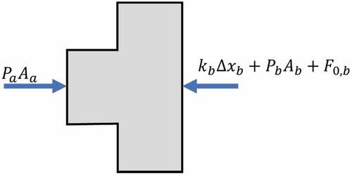
where $P_a$ and $P_b$ are air pressures; $A_a$ and $A_b$ are pressured applied areas; $k_b$ is spring stiffness; $\mathrm{\Delta }{x}_b$ is spring deflection or block displacement; and $F_{0,b}$ is spring preload. This model uses a quasistatic assumption and neglects the inertia of the moving block. By knowing air pressures at both sides and other valve parameters, valve motion ($\mathrm{\Delta }{x}_b$) can be easily determined using Equation (63)(63) $P_a{A}_a=k_b\mathrm{\Delta }{x}_b+P_b{A}_b+F_{0,b}$(63) . Displacements calculated using this model also need to be adjusted by two other physical limitations: (1) when $\mathrm{\Delta }{x}_b$ is less than zero, $\mathrm{\Delta }{x}_b$ is set to be zero and (2) when $\mathrm{\Delta }{x}_b$ is greater than its maximum value, $\mathrm{\Delta }{x}_b$ is set to be its maximum value. Having determined the valve motion, the corresponding orifice opening size is proportional to the displacement.

Abdol-Hamid [52] also developed a locomotive relay valve model in which inertial properties and variable moving masses were considered, i.e., a dynamics model. To keep the present paper concise, the example shown in Figure 9 is used again to discuss the relay valve model:

(64) $P_a{A}_a-\left(k_b\mathrm{\Delta }{x}_b+P_b{A}_b+F_{0,b}\right)=m_{bk}{a}_{bk}$(64)

where $m_{bk}$ is the mass of the block and $a_{bk}$ is the acceleration of the block. The mass of the block can change when the current block comes in contact with other blocks and then they move together. For example, in the AAR 26 C locomotive brake system, the diaphragm-rod block can be in contact with supply and/or exhaust valve blocks to form different combinations of mass blocks. To solve this equation, a numerical integrator is needed. Both quasistatic and dynamic models can be used to simulate valve motions. Obviously, quasistatic models are much easier to solve. However, the dynamic models have the advantage of being able to describe the transitions of valve actions more accurately and are better models for valve designs.

Note that Equation (63)(63) $P_a{A}_a=k_b\mathrm{\Delta }{x}_b+P_b{A}_b+F_{0,b}$(63) and ((64) are two simple examples of quasistatic and dynamic valve motion models. Following the same principles, more elements can be added into the model, for example, multiple-pressure bearing surfaces, multiple springs and multiple mass blocks. When brake valves are positioned vertically, gravitational forces can also be added. Murtaza and Garg [118] developed a dynamics valve motion model to simulate Indian air brake systems. Dynamic valve models were also developed by Bubnov [115] in his PhD thesis. Quasistatic valve motion models were used in [81,94,101].

It is worth mentioning that, by using commercial software packages such as the AMESim, more elements can be added into the valve motion model. For example, in references [102–105], friction forces and vicious damping have been added to valve motion models. Wu et al. [101] developed a n in-house air brake model in which friction forces and viscous damping were also considered. Specifically, when the sum of external forces is no greater than the friction force, the studied block remains still. The consideration of viscous damping was achieved by limiting the velocity of a moving block to an empirical maximum value.

4.4.3. Orifice models

Previously reviewed valve motion models are able to determine connections and disconnections of various components; they should also determine the opening sizes of the connections. The next task is to develop orifice models and determine the status of air flows.

Abdol-Hamid [52] reviewed two different models for square edged orifices and sharp edged orifices (see Figure 10(a)). Modelling of the former was expressed as:

(65) $=\left\{\begin{array}{cc}0.8\sqrt{\frac{2\left({\left(\frac{P_{up}}{P_{dn}}\right)}^{-2/\gamma }-{\left(\frac{P_{up}}{P_{dn}}\right)}^{-\left(\gamma +1\right)/\gamma }\right)}{\left(\gamma -1\right)RT}}{A}_r{P}_{up}& \frac{P_{up}}{P_{dn}}<1.89,subsonic\\ 2.367A_r{P}_{up}& \frac{P_{up}}{P_{dn}}\ge 1.89,supersonic\end{array}\right.$(65)

Figure 10. Orifices: (a)square and sharp edged orifices and (b) orifice flow [48].

where ${\dot{m}}_r$ is orifice flow rate; $P_{up}$ is the upstream pressure; $P_{dn}$ is the downstream pressure; $\gamma$ is specific heat ratio and $A_r$ is the orifice area. Modelling of the sharp edged orifice was expressed as:

(66) ${\dot{m}}_r=0.6{\bar{A}}_r{P}_d\sqrt{\frac{{\left(\frac{P_{up}}{P_{dn}}\right)}^2-1}{RT}}\frac{\left|\frac{P_{up}}{P_{dn}}-1\right|}{\frac{P_{up}}{P_{dn}}-1}$(66)

(67) ${\bar{A}}_r=\frac{1}{\sqrt{\left(1/A_{up}^2\right)+\left(1/A_{dn}^2\right)}}=\frac{A_{up}{A}_{dn}}{\sqrt{A_{up}^2+A_{dn}^2}}$(67)

where $A_{up}$ is the orifice area at upstream; $A_{dn}$ is the orifice area at downstream; ${\bar{A}}_r$ is the equivalent orifice area. According to Abdol-Hamid [52], results calculated using these two orifice models had about 10% differences that were acceptable for engineering applications. However, the sharp edge orifice model does not need to differentiate subsonic or sonic flow. The latter model was used in [52,60,63].

Pugi et al. [71] modelled orifice flows as:

(68) ${\dot{m}}_r=A_r{\delta }_q{\delta }_M\frac{P_{up}}{\sqrt{T_{up}}}$(68)

(69) ${\delta }_M=\left\{\begin{array}{cc}\sqrt{\frac{2\gamma }{R\left(\gamma -1\right)}}\sqrt{\left({\left(\frac{P_{dn}}{P_{up}}\right)}^{2/\gamma }-{\left(\frac{P_{dn}}{P_{up}}\right)}^{\left(\gamma +1\right)/\gamma }\right)}& subsonic\\ \sqrt{\frac{\gamma }{R}{\left(\frac{2}{\gamma +1}\right)}^{\left(\gamma +1\right)/\gamma -1}}& supersonic\end{array}\right.$(69)

(70) ${\delta }_q=0.8414-0.1002\left(\frac{P_{dn}}{P_{up}}\right)+0.8415{\left(\frac{P_{dn}}{P_{up}}\right)}^2-3.9{\left(\frac{P_{dn}}{P_{up}}\right)}^3+4.6001{\left(\frac{P_{dn}}{P_{up}}\right)}^4-1.6827{\left(\frac{P_{dn}}{P_{up}}\right)}^5$(70)

where are ${\delta }_M$ and ${\delta }_q$ are two correction parameters. It can be seen that this model is essentially the same as the model expressed by Equation (65)(65) $=\left\{\begin{array}{cc}0.8\sqrt{\frac{2\left({\left(\frac{P_{up}}{P_{dn}}\right)}^{-2/\gamma }-{\left(\frac{P_{up}}{P_{dn}}\right)}^{-\left(\gamma +1\right)/\gamma }\right)}{\left(\gamma -1\right)RT}}{A}_r{P}_{up}& \frac{P_{up}}{P_{dn}}<1.89,subsonic\\ 2.367A_r{P}_{up}& \frac{P_{up}}{P_{dn}}\ge 1.89,supersonic\end{array}\right.$(65) . The subsonic part of Equation (69)(69) ${\delta }_M=\left\{\begin{array}{cc}\sqrt{\frac{2\gamma }{R\left(\gamma -1\right)}}\sqrt{\left({\left(\frac{P_{dn}}{P_{up}}\right)}^{2/\gamma }-{\left(\frac{P_{dn}}{P_{up}}\right)}^{\left(\gamma +1\right)/\gamma }\right)}& subsonic\\ \sqrt{\frac{\gamma }{R}{\left(\frac{2}{\gamma +1}\right)}^{\left(\gamma +1\right)/\gamma -1}}& supersonic\end{array}\right.$(69) is the same as the square root part of Equation (65)(65) $=\left\{\begin{array}{cc}0.8\sqrt{\frac{2\left({\left(\frac{P_{up}}{P_{dn}}\right)}^{-2/\gamma }-{\left(\frac{P_{up}}{P_{dn}}\right)}^{-\left(\gamma +1\right)/\gamma }\right)}{\left(\gamma -1\right)RT}}{A}_r{P}_{up}& \frac{P_{up}}{P_{dn}}<1.89,subsonic\\ 2.367A_r{P}_{up}& \frac{P_{up}}{P_{dn}}\ge 1.89,supersonic\end{array}\right.$(65) , and the supersonic part of Equation (69)(69) ${\delta }_M=\left\{\begin{array}{cc}\sqrt{\frac{2\gamma }{R\left(\gamma -1\right)}}\sqrt{\left({\left(\frac{P_{dn}}{P_{up}}\right)}^{2/\gamma }-{\left(\frac{P_{dn}}{P_{up}}\right)}^{\left(\gamma +1\right)/\gamma }\right)}& subsonic\\ \sqrt{\frac{\gamma }{R}{\left(\frac{2}{\gamma +1}\right)}^{\left(\gamma +1\right)/\gamma -1}}& supersonic\end{array}\right.$(69) is also a constant. Equations (68)(68) ${\dot{m}}_r=A_r{\delta }_q{\delta }_M\frac{P_{up}}{\sqrt{T_{up}}}$(68) and (69(69) ${\delta }_M=\left\{\begin{array}{cc}\sqrt{\frac{2\gamma }{R\left(\gamma -1\right)}}\sqrt{\left({\left(\frac{P_{dn}}{P_{up}}\right)}^{2/\gamma }-{\left(\frac{P_{dn}}{P_{up}}\right)}^{\left(\gamma +1\right)/\gamma }\right)}& subsonic\\ \sqrt{\frac{\gamma }{R}{\left(\frac{2}{\gamma +1}\right)}^{\left(\gamma +1\right)/\gamma -1}}& supersonic\end{array}\right.$(69) ) were developed with the isentropic assumption; then Equation ((70) was used as a correction parameter to indirectly consider the effects of adiabatic flows. Another orifice model that has essentially the same mathematical expressions can be found in [48]. The contribution of reference [48] in this regard is the introduction of another correction parameter to consider that the effective cross-sectional area of the orifice is smaller than its physical area due to the continuity of the flow path as shown in Figure 10(b).

Piechowiak [81] modelled adiabatic orifice flows as:

(71) ${\dot{m}}_r={\left(\frac{\gamma +1}{2}\right)}^{1/\left(\gamma -1\right)}{\epsilon }^{1/\gamma }\sqrt{\frac{\gamma +1}{\gamma -1}\left[1-{\epsilon }^{\left(\gamma -1\right)/\gamma }\right]}{\epsilon }_{\ast }{A}_r\sqrt{\gamma P_{up}{\rho }_{up}}{\left(\frac{2}{\gamma +1}\right)}^{\gamma +1/2\left(\gamma -1\right)}$(71)

where $\epsilon$ and ${\epsilon }_{\ast }$ are two parameters that are related to orifice geometry; and ${\rho }_{up}$ is the upstream air density. In addition to this adiabatic model, Piechowiak [81] recommended to use a simple model to simulate orifice flows when pressure differences are small:

(72) ${\dot{m}}_r={\delta }_f\left(P_{up}-P_{dn}\right)$(72)

where ${\delta }_f$ is a simple parameter that considers laminar friction. Similar model was used by Bharath et al. [68] to determine mass flow rate between reservoirs and brake cylinders.

Wu et al. [101] followed a fluid dynamics model used for automotive engines and modelled air flow between two volumes as

(73) $\begin{array}{rl}& {\dot{m}}_r=\left\{\begin{array}{c}\frac{P_{up}{A}_r}{v_{s,up}}{\left\{\left(\frac{2{\gamma }^2}{\gamma -1}\right){\left(\frac{P_{dn}}{P_{up}}\right)}^{2/\gamma }\left[1-{\left(\frac{P_{dn}}{P_{up}}\right)}^{\left(\gamma -1\right)/\gamma }\right]\right\}}^{\frac{1}{2}}\frac{P_{dn}}{P_{up}}>{\left(\frac{2\gamma }{\gamma +1}\right)}^{\frac{\gamma }{\gamma -1}}subsonic\\ \frac{P_{up}{A}_r}{v_{s,up}}\gamma {\left(\frac{2}{\gamma +1}\right)}^{\left(\gamma +1\right)/\left[2\left(\gamma -1\right)\right]}\frac{P_{dn}}{P_{up}}\le {\left(\frac{2\gamma }{\gamma +1}\right)}^{\frac{\gamma }{\gamma -1}}supersonic\end{array}\right.\\ & \\ & \end{array}$(73)

where $v_{s,up}$ is the speed of sound at upstream. After some basic mathematic transformations, one can find that Equation (73) is the same as Equation (68)(68) ${\dot{m}}_r=A_r{\delta }_q{\delta }_M\frac{P_{up}}{\sqrt{T_{up}}}$(68) but the former does not have the correction parameters for adiabatic flow.

4.4.4. Fixed and variable volumes

Having determined the mass flow rates of all inlets and outlets, the next step of brake system simulations is to determine the pressure changes in various volumes. These volumes can be fixed volumes or variable volumes. Fixed volumes can be reservoirs, chambers, small bulbs, etc., whilst variable volumes mostly refer to brake cylinders. Brake valves with pistons and diaphragms can also be modelled with variable volumes. However, volume variations in brake valves due to the movements of pistons and diaphragms are usually small and have negligible implications to the overall simulation results; these small volumes are therefore often modelled as fixed volumes and are combined to nearby larger volumes as small additional volumes. For example, a small variable volume in a brake valve can be combined to an auxiliary reservoir (when the small volume is connected to the auxiliary reservoir) by adding a small volume to the fixed volume of the auxiliary reservoir.

Modelling pressure changes in fixed volumes is straightforward and follows:

(74) $\dot{P}=RT\dot{m}/V$(74)

Obviously, it is a derivation of the ideal gas law ($PV=mRT$). This model is universally used across almost all air brake studies. Piechowiak [81] has considered pressure changes due to heat transfers. In this case, heat transfers from atmosphere to reservoir wall, and from reservoir wall to pressurized air need to be calculated. Having determined these heat transfers, by knowing the mass of the pressurized air, temperature changes and pressure changes of the pressurized air can be obtained.

Compared to fixed volume models, variable volume (brake cylinder) models are more complex. The early model reported by Abdol-Hamid [52] had already considered many features including minimum piston travel (minimum cylinder volume), return spring stiffness, return spring preload and maximum piston travel (maximum cylinder volume). It is a quasistatic model; when cylinder volume is greater than the minimum volume and less than the maximum volume, the value is determined similarly to the process shown in Figure 9 for valve motions; friction, viscous damping and piston mass were not considered. In Abdol-Hamid’s model, piston position was redetermined for each time step, then Equation (74)(74) $\dot{P}=RT\dot{m}/V$(74) was used with the current cylinder volume to determine cylinder pressure.

Bharath et al. [68] modelling cylinder piston as a dynamic body:

(75) $M_{ps}{\ddot{x}}_{ps}+c_{ps}{\dot{x}}_{ps}+k_{ps}{x}_{ps}=\left(P_{ps,1}-P_{ps,2}\right)A_{ps}$(75)

where $M_{ps}$ is the piston mass; $x_{ps}$ is the piston displacement; $c_{ps}$ is the viscous damping; $k_{ps}$ is the equivalent spring stiffness; $A_{ps}$ is the piston pressure; and $P_{ps,1}$ and $P_{ps,2}$ are pressures applied at two sides of the piston. Full dynamics piston models were also used by Teodoro et al. [107], a Runge-Kutta method was used by Bharath et al. [68] to solve the dynamics equations and a Euler method was used in [107]. Pugi et al. [71] also modelled the dynamics of brake cylinder pistons; in their model, an extra force of spring preload was considered. Having determined the displacement of cylinder piston, cylinder pressures were expressed as:

(76) $P_b=\frac{1}{x_{ps}\left(t\right)}\left(x_{ps,0}{P}_{b,0}+\frac{1}{RT{A}_{ps}}\underset{0}{\overset{t}{\int }}\dot{m}\left(t\right)dt\right)$(76)

where $P_b$ is the cylinder pressure; $x_{ps,0}$ is the initial displacement of the piston and $P_{b,0}$ is the initial pressure of the cylinder. Another dynamic brake cylinder piston model was developed by Bubnov [115]. It is worth mentioning that dynamics piston models can also be developed by using the commercial software package AMESim as used in [102–105].

Afshari et al. [63] expressed pressure changes in brake cylinders as:

(77) $\dot{P}=\left(RT\dot{m}-P\dot{V}\right)/V$(77)

This is another derivation from the ideal gas law ($PV=mRT$) by assuming that both mass flow and volume are functions of time. The volume changing rate can be obtained using quasistatic methods as used by Abdol-Hamid [52] or the dynamics method as expressed by Equation (75)(75) $M_{ps}{\ddot{x}}_{ps}+c_{ps}{\dot{x}}_{ps}+k_{ps}{x}_{ps}=\left(P_{ps,1}-P_{ps,2}\right)A_{ps}$(75) . A similar model as Equation (77)(77) $\dot{P}=\left(RT\dot{m}-P\dot{V}\right)/V$(77) was used by Piechowiak [81] to model an adiabatic cylinder (a parameter of ratio of specific heats was added). Piechowiak [81] also presented a second brake cylinder model that had more details, in which the cylinder pressure was expressed as:

(78) $P_b{A}_{ps}=F_{ps,0}+F_f\left({\dot{x}}_{ps},P_b\right)+k_{ps}{x}_{ps}+c_{ps}\left(P_b\right){\dot{x}}_{ps}$(78)

(79) ${\dot{P}}_b=\frac{\gamma -1}{V}\dot{q}+\dot{m}\frac{\gamma }{V}RT-\frac{\gamma }{x_{ps,0}+x_{ps}}{\dot{x}}_{ps}$(79)

where $F_f$ is a friction force that is related to piston speed and cylinder pressure; $c_{ps}$ is a viscous damping that is related to cylinder pressure; and $\dot{q}$ is the heat exchange rate. It can be seen that this model has now considered cylinder spring preload, friction force, viscous damping force and heat exchange.

Wu et al. [101] developed a brake cylinder model as:

(80) $\stackrel{=}{P_b}\frac{v_{s,up}^2\dot{m}}{V}-\gamma P_b\dot{V}=\frac{v_{s,up}^2\dot{m}}{V}-\gamma P{A}_{ps}\mathrm{\Delta }{x}_{ps}$(80)

(81) $\dot{V}=A_{ps}\mathrm{\Delta }{x}_{ps}={\dot{P}}_b{A}_{ps}^2/k_{ps}$(81)

Using these two equations, pressure change rate (${\dot{P}}_b$), volume change rate ($\dot{V}$) and piston displacement change ($\mathrm{\Delta }{x}_{ps}$) can be approximated. Then the external force applied on the piston was assessed to determine if the piston change is used or not. If external force is less than static friction, the displacement change will not be applied.

5. Brake rigging and brake shoe (pad) friction

Having determined pressures in brake cylinders, the next step of brake simulation is to convert cylinder pressures to normal forces on brake shoes (or pads) and then to friction forces (or torques) applied on wheels. The conversion from cylinder pressures to brake normal forces is achieved via brake rigging setups. A simplified diagram of brake rigging is shown in Figure 11 where a simple lever is used. In reality, brake rigging is a system of levers and has more complicated mechanisms [48,119]. The arrangement and the layout of the brake rigging can be different when following different standards. Descriptions of some typical North American riggings can be found in [120]. The UIC544-1 Leaflet [121] describes typical riggings that are commonly used in Europe. Brake riggings can also be classified as body mounted and track mounted brake riggings [120]. The former commonly uses one brake cylinder and rigging components are mostly mounted underneath the chassis and provide brake forces to both bogies whilst the latter can use up to two brake cylinders and two less complicated copies of riggings are used to provide brake forces to two bogies respectively.

Figure 11. Brake rigging and wheel-rail adhesion, where $F_{ad}$ is the adhesion force; $r_w$ is wheel radius; $v_{st}$ is wheel translational speed; $\omega$ is wheel rotational speed; $N_b$ is brake shoe normal force; $F_b$ is brake shoe friction force; and $P_b$ is brake cylinder pressure.

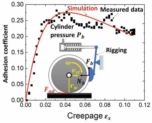
In most brake simulations, friction forces generated from brake shoes ($F_b$ in Figure 11) is used as the brake forces with the assumption that wheel-rail adhesion can provide sufficient tangential forces in wheel–rail interfaces. Martin and Hay [16] calculated brake forces as:

(82) $F_b=\frac{P_{b,t}}{P_{b,max}}{\delta }_{bm\mathrm{\%}}{m}_{car}{\delta }_{total}{\mu }_b$(82)

where ${\delta }_{bm\mathrm{\%}}$ is the brake mass percentage; ${\delta }_{total}$ is the total efficiency of the brake system; and ${\mu }_b$ is the brake shoe Coefficient of Friction (CoF). In reference [7], brake forces were determined as:

(83) $F_b=\left\{\begin{array}{cc}0& P_b<10psi\\ \left(0.025P_b-0.25\right){\mu }_b& P_b>10psi\end{array}\right.$(83)

The model considered the cylinder spring actions and movements of the cylinder piston. When cylinder pressure is little than 10 psi, brake shoes do not press on wheels due to spring forces and piston travels. When cylinder pressure is greater than 10 psi, the normal forces ($N_b$) were modelled as proportional to cylinder pressure with a factor of 0.025.

The most common model used to convert brake pressure to brake forces in open literature can be expressed as:

(84) $F_b=\left(P_b{A}_{ps}-F_{ps}\right){\mu }_b{\delta }_{rigging}{\delta }_{efficiency}{\delta }_{adhesionlimit}{n}_b\frac{r_b}{r_w}-F_f$(84)

where $A_{ps}$ is the cylinder cross-sectional area; $F_{ps}$ is cylinder spring force; ${\delta }_{rigging}$ is rigging factor; ${\delta }_{efficiency}$ is system efficiency coefficient; ${\delta }_{adhesionlimit}$ adhesion limiting factor; $n_b$ is the number of brake cylinder or number of brake discs; $r_b$ is effective brake radius for disc brake; $r_w$ is wheel radius; and $F_f$ is cylinder piston friction. Brake force calculations are also documented in standards such as [121–123].

Equation (84)(84) $F_b=\left(P_b{A}_{ps}-F_{ps}\right){\mu }_b{\delta }_{rigging}{\delta }_{efficiency}{\delta }_{adhesionlimit}{n}_b\frac{r_b}{r_w}-F_f$(84) is a general expression for brake force calculations. Variations exist in different publications. Presciani et al. [6] used the adhesion limiting factor to consider degraded wheel-rail adhesion condition; specifically, 95% was used for degraded adhesion condition. Lee and Kang [11] directly calculated brake torques applied on wheel discs, therefore effective brake radius ($r_b$) and number of brake discs ($n_b$) were considered. References [42,71] included $n_b\frac{r_b}{r_w}$ to simulate brake forces. Aboubakr and Shabana [62] considered cylinder piston friction for their brake force model.

Brake shoe CoFs have usually have different expressions for different materials, a number of examples are given as:

(85) ${\mu }_b=0.82\frac{N_b+100}{7N_b+100}\frac{17v_{km}+100}{60v_{km}+100}+0.0012\left(120-v_{km0}\right)$(85)

(86) ${\mu }_b=0.41\frac{N_b+200}{4N_b+200}\frac{v_{km}+150}{2v_{km}+150}$(86)

(87) ${\mu }_b=0.475\frac{2v_{km}+40}{5v_{km}+40}$(87)

where $N_b$ is the brake shoe normal force; $v_{km}$ is the speed of the vehicle in km/h; and $v_{km0}$ is the initial speed of the vehicle in km/h. Three CoFs equations have considered different influencing factors. The third equation considers vehicle speed only; the second equation considers normal forces applied on wheels as well; and the first equation has added the initial speed of the vehicle into consideration.

6. Wheel-rail adhesion in brake models

As mentioned previously, most brake simulations use brake shoe friction forces ($F_b$ in Figure 11) as the final brake forces. However, it is noted that the actual and meaningful brake forces applied on wheels or vehicles are the adhesion forces generated from wheel-rail interfaces ($F_{ad}$ in Figure 11). The simplification of using friction forces as brake forces is correct and accurate when the following condition is met:

(88) $F_b\le Q_{car}{\mu }_d=F_{ad}$(88)

where $Q_{car}$ is the normal force applied from the wheel to the rail; and ${\mu }_d$ is the dynamic adhesion coefficient that is related to the longitudinal creepage at wheel–rail interface:

(89) ${\epsilon }_x=\frac{r_w\omega -v_{st}}{v_{st}}$(89)

When brake shoe friction force is greater than adhesion force, wheel skidding or wheel sliding will occur. In this case, the actual brake forces are then smaller than brake shoe friction forces. For example, Presciani et al. [6] used a 95% adhesion limiting factor for simulations that had degraded adhesion conditions. As reviewed by Wu et al. [124], most LTD simulations have an adhesion limit applied to brake forces and traction forces. The adhesion limit can be speed dependent and track location dependent.

Considering the relationship between brake shoe friction forces and actual brake forces, i.e., wheel rail adhesion forces, brake models that consider wheel-rail adhesion have greater simulation capabilities. In a brake study carried out by Lee and Kange [11], a 2D vehicle model that has three Degrees of Freedom (DoFs) for each body was developed. The Hertz theory and Polach model were used to determine wheel-rail adhesion forces and eventually brake forces. Researchers in [125–128] have studied implications of brake forces to vehicle dynamics. The focus of these studies was vehicle dynamics and therefore the brake models were very simplified. Shrestha et al. [129] reviewed various other brake-related studies that had a focus on wheel-rail adhesions.

Wu et al. [45] introduced a wheel-rail adhesion model into a full train brake model. In this model, each individual wagon of the train was modelled in 2D with the consideration of wheel-rail contact and frictional suspensions. The Hertz theory and Polach model were used again for the wheel-rail contact model. The train model was solved by using a Parallel Computing technique. An interesting result that was obtained by Wu et al. [45]. is shown in Figure 12 which indicates that the wheel-rail adhesion force, i.e., the actual brake force, is smaller than the brake shoe friction force. The force difference was used to generate declaration for wheelset rotational speed. To match the results of using LTD simulations and 2D train dynamics simulations, influences of wheelset rotational inertia need to be converted to extra mass of the vehicle and considered in LTD simulations.

Figure 12. Brake simulations with wheel-rail adhesion [45].

7. Challenges and research gaps in brake modelling

To spark new ideas in this research field, this section discusses challenges and research gaps in brake modelling, as well as various other brake study-related issues.

7.1. Model fidelity and computational efficiency

When selecting an air brake model or developing a new model for relevant research, the balance between model fidelity and computational efficiency is one of the most common issues. This section discusses several issues in this regard.

7.1.1. Computing speed versus complexity

Models with high fidelity, e.g., fluid dynamics models, commonly have higher model complexity and lower computational speeds. Empirical models, on the other hand, have lower fidelity but are much easier to develop and oftentimes have significantly faster computing speeds. Simulation experience indicates that a fluid dynamics air brake model can be 100 times slower than its empirical counterpart. Real-time fluid dynamics air brake models are rare but almost all empirical air brake models are faster than real-time. Knowing that the slow computational speed is the main disadvantage of fluid dynamics air brake models, some studies have been focused on this disadvantage. Recent advances reported from Dalian Jiaotong University (China) have achieved real-time simulations on quality desktops (CPU clock speed 3.6 GHz or higher) without parallel computing for air brake systems of DP trains (e.g., 1 locomotive + 108 wagons + 1 locomotive +108 wagons).

In addition to low computational speeds, high model complexity is the second challenge of using fluid dynamics models. Fluid dynamics models require simulation of air flows in brake pipes, brake valves and various volumes. Simulations of these air flows and connections among various components are complex as reviewed in this paper.

7.1.2. Selection of brake models

Selection of air brake models should fit the objective of the research. For example, equivalent constant force models as one of the most simplified brake models are often used in signalling design to approximate train braking distances. All other types of empirical models reviewed in this paper have been used in train dynamics simulations, typically in LTD simulations. This is very popular, especially when faster computing speeds are desired and air brake system behaviour is not of particular interest. One justification that is often used is that air brake system behaviour has significant implications for train dynamics but not the other way. Air brake system behaviour can therefore be regarded as prescribed inputs.

While using empirical models, one often used assumption is that the measured air brake behaviour of a longer train can cover that of a shorter train. For example, researchers often use brake behaviour of wagon 001 to wagon 050 measured from a 100 wagon consist to represent that of a train with only 50 wagons. This assumption is understandable and very practical as brake tests are often not able to be performed on all configurations due to time and cost limits. However, it is noted that, when two train consists are significantly different in total lengths, brake behaviour of the shorter consist can be considerably different from that of the longer consist. An interesting research topic can be developed to understand the limit of length differences when this assumption can be safely applied.

The differences in brake systems of long and short train consists mainly originate from the dynamic behaviour of brake pipes. Therefore, the assumption discussed in the previous paragraph can be solved by using fluid or fluid-empirical air brake models. It can also be said that the differences in brake behaviour between a 50 wagon consist and a 100 wagon consist should be captured by a fluid dynamics or a fluid-empirical brake model. Considering that fluid dynamics models have lower computational speeds and are not desired when faster train dynamics simulations are required, fluid-empirical models seem to be a more suitable option to strike a balance between model fidelity and computational speeds. Another good approach to address the previously discussed assumption is to simulate brake behaviour of a specific wagon consist using a fluid dynamics model and then use the air brake simulation results to update an empirical air brake model that can be used in train dynamics simulations.

In addition to the flexibility advantage of fluid dynamics models, an irreplaceable advantage of fluid dynamics models is their descriptions of brake system components (pipes, connections, valves, pistons, etc.). Simulations of these components can provide more direct recommendations for brake system designs. Some studies such as the simulations of Undesired Emergency Brake can only be done using detailed fluid dynamics models. Fluid dynamics models are better options when air brake system behaviours are often the issue of particular interest. Brake availability is another topic that requires fluid dynamics models. For example, in-service simulations considering reservoir refilling and availability for consecutive brake applications, and the likely consequences of delayed refilling.

It is noted that model fidelity is more related to model versatility or flexibility but not necessarily determining model accuracy. As discussed previously, high-fidelity models such as fluid dynamics models are more versatile and can have the capability to simulate trains that the models were not validated with during the development stages. However, there is a risk that empirical models may not be accurate in such cases. For braking scenarios that have sufficient data for model validations, model accuracy is not dependent on model fidelity. In other words, empirical models can be as accurate as the fluid dynamics models for simulation cases where measured data are sufficient.

7.1.3. Mesh sizes of fluid dynamics models

Mesh sizes of brake pipes (Table 2) also have evident implications for simulation results. Finer meshes or smaller mesh sizes enable better simulations of propagation of pressure waves. This is important for models to capture high-frequency phenomena such as the activation of the quick action bulb in brake valve distributors. There should be a limit regarding what size of mesh is required to allow the model to correctly capture these pressure wave propagations. In practical brake modelling, models that have large mesh sizes often need to adjust pipe wall friction (sometimes to unrealistic values) to allow simulation results to match experimental data. However, it has to be pointed out that there should be a balance with computing speed as smaller mesh sizes mean larger models and longer simulations time.

7.1.4. Brake models in railway network simulations

Brake models are important parts of railway network simulations where the movements of multiple trains need to be considered at the same time. Network simulations are of interest not only for planning purposes but also for energy savings. Varying in the levels of details, network simulations can be divided into two groups: discrete [130,131] and continuous [132,133]. Regardless of the modelling methods, brake models in railway network simulations are usually very simplified by using constant or equivalent constant brake forces. Researchers have expressed interests in improving brake models by adding more details. However, the extra details cannot be achieved by using simplified train models. Models to the complexity levels of LTD models are often required to effectively reflect the details of the air brake models. This again raises the computational efficiency issue as LTD models are regarded as slow in this case. Furthermore, the considerations of mechanical parameters in LTD models make it difficult to integrate these models into complex frameworks (such as transport simulation software and smartphone applications). Therefore, there is a need to develop novel and simple brake models and train dynamics models for effective applications in traffic engineering.

7.1.5. Parallel computing

Parallel computing uses multiple-computer cores to process multiple computing tasks simultaneously. The obvious motivation and advantage of using parallel computing is to improve computing speeds. Parallel computing for air brake simulations has been reported by Wu et al. [101] and Teodoro et al. [108]. Two studies used two different parallel computing techniques respectively: Message Passing Interface and Open Multi-Processing. As discussed in Wu et al. [134], these two techniques are different in memory and information sharing. However, both studies partitioned the simulated brake systems in similar ways. Specifically, brake models were partitioned into wagon groups or individual wagons; then the models were linked via the hose connections. This is intuitively understandable as, in reality, brake equipment on individual wagons can be regarded as independent units that are communicating via hose connections. Wu et al. [101] reported 70% of reduction in computing time by using four computer cores while Teodoro et al. [108] reported more than 80% reduction in computing time by using six or eight computing cores. These results are also good examples to show that computing time reductions are not proportional to the number of computing cores that are used. When more computer cores are used, more time is used for communication among parallelized computer cores. Situations are possible when more computer cores are used, the overall computing time increased due to excessive overhead of communications. Therefore, optimal parallel computing scheme for air brake simulations is a valuable research question.

7.2. Determination of model parameters

A brake model has a lot of parameters and models with higher fidelity often have more model parameters. It has been noticed that the determination of air brake model parameters, for both empirical and fluid dynamics models, has been a challenge due to several reasons. Constant force models and look-up table models probably have the least number of parameters needing to be determined; however, they require the support of sufficient experimental data. Other types of empirical models require tuning parameters to allow empirical formulas to fit experimental data. Models with a small number of (e.g., one or two) tuning parameters can be tuned manually. Iterative tuning and curve fitting tools may be required for models that have many (e.g., more than three) tuning parameters. Typically, for empirical models, key model parameters that need to be determined include brake/release delays, pressure changing rates or fitting functions, and steady-state pressures. Those parameters are usually different at different brake and release scenarios, e.g., minimum service brake, maximum service brake, emergency brake and their releases. And multiple parameters are required depends on different forms of fitting functions, e.g, power functions, exponential functions, and polynomial functions.

For fluid dynamics models, the challenge mainly comes from two aspects: information availability and unmodeled details. Some model parameters, such as orifice diameters, spring stiffness and piston travels, are not known to the researcher due to commercial confidentiality. Under such situations, empirical data and reverse-engineering have to be used and the resulting model parameters may not be the accurate data. During air brake modelling, many other parameters, such as valve sliding friction, pipe wall friction, and system damping, are not able to be measured. The values of these parameters are mainly approximated by following theoretical formulas such as the Darcy-Weisbach Equation or by using empirical values. These approximations inevitably introduce errors to the model. The second aspect, i.e., unmodelled details, refers to the details that are not practical to be included in the model but have influences on the simulation results. For example, Cruceanu [48] pointed out that the effective diameter of an orifice can be smaller than its physical diameter due to the continuity of air flows. In this case, even if the researcher has the data of orifice diameter, the final model still has noticeable errors as details of flows passing through the orifice are not practical to be modelled in air brake simulations. Such situations are quite common in air brake modelling as the exact model parameters are often not able to be used in final models. Slight increases or decreases of the exact parameters are often needed to allow good matching with validation data. Another good example is the modelling of connection pipes between an auxiliary reservoir and the main brake valve. Researchers may find that they need to slightly increase the volume of the auxiliary reservoir to achieve better results. This is mainly due to the small volume of the connection pipe which is also too computationally costly to be modelled with comprehensive details.

Typically, for fluid dynamics models, key parameters include pipe diameters, pipe wall friction, connection friction, various orifice diameters, orifice friction, valve spring stiffness, valve friction and effective volumes of various reservoirs and chambers. Note that depends on different levels of model fidelity, the parameter list varies significantly. With many model parameters to be determined, especially for fluid dynamics models, manual tuning is very time-consuming. Parameter identification algorithms (e.g. [135],) and iterative parameter tuning algorithms are good research topics.

7.3. Further detailed brake system modelling

Most brake pipe models do not use the energy conservation equation and do not consider heat transfers in brake operations. Models that have considered heat transfers have rarely studied temperature variations in brake pipes. Piechowiak [81] has presented a short discussion in this regard. It is known that temperature changes in brake pipes can change the speed of sound (propagation speeds of pressure waves) and then change brake and release delays. Research into such temperature changes in brake pipes and even in brake valves and various volumes can be interesting. The same research directions can also be applied to the influences of humidity in brake pipes and valves.

Undesired Emergency Brake (UDE) application studies have been undertaken since the 1980s. However, UDE simulations are still rare. The early model developed by de Leon and Limber [59] considered the movements of the vehicles resulting in air sloshing in brake pipes. Better brake pipe models require the consideration of inter-vehicle impacts and deformation of brake pipes. Design improvements of brake valves have evidently decreased the occurrences of UDE events. However, they are not solved and are still being reported in recent years. Research into this direction is of great engineering interest and research value.

Different types of orifices are used in air brake systems, e.g., sharp-edged, square-edged and concentric orifices. Normally, air brake models do not differentiate these orifices. Abdol-Hamid [52] stated that sharp-edged and square-edged orifice models can have 10% differences in results. Further investigations into the implications of these orifices for brake valve behaviour and air brake simulation results can be interesting.

The literature review carried out for writing this paper shows that dynamics simulations of valve motions are still challenging. Models that consider inertia and acceleration of various valves are rare and dynamics models for whole distributor valves, which may include regulating valves, emergency valves, quick-release valves, etc., are even less in number. Yang [103] developed such a dynamics model for a distributor valve using AMESim. However, such models have not been reported from in-house codes.

Brake simulations with the consideration of wheel-rail adhesion will become a popular topic for future studies. Such simulations require the addition of wheel-rail contact models, especially the creep force models [136] and brake processes can involve large creepages at which the creep forces have the ‘falling’ feature. This falling feature was observed from field testing in which creep forces first increased with creepages but then decreased at large creepages after creep forces reach a certain maximum value. Simulations of such a falling feature is important for brake force studies. For such studies, the Polach model [137] and modified Fastsim [138] are recommended considering their falling feature simulation capability and computational speeds. It can be argued that, under normal operational conditions, the phenomenon of failing friction is more of an issue for traction than braking considering the significantly smaller forces involved with braking (e.g., 0.2 kN per tonne for wagons) than with traction (e.g., 3 kN per tonne for locomotives). Therefore, the failing friction feature is less important if wheel slides are not present. However, for situations where Wheel Sliding Protection (WSP) is required, the failing friction feature becomes necessary. More discussions about WSP will be presented later in this section.

7.4. The use of commercial software packages

Detailed simulations of railway air brakes are still a quite specialized research topic that is confined to a small number of academic and industrial groups. These in-house codes are often an accumulation of many years of research; and the development requires time, knowledge and experience. Commercial software packages such as AMESim and Matlab-Simulink offer great modelling capabilities that can significantly reduce the time investment for researcher who do not have access to legacy codes. However, it has to be pointed out that technical information about air brake systems and specific know-how of air brake modelling are critical for air brake research regardless of the utilization of in-house or commercial software packages.

Fluid dynamics air brake models developed by using commercial software packages also have the issue of low computational speeds. And the biggest disadvantage of using commercial software package is probably their incompatibility with other train dynamics simulation models. Communications between such air brake models and train dynamics models require the development of a co-simulation interface which can be a significant extra cost.

7.5. Modularized air brake modelling

As discussed previously, there are many uncertainties in air brake model parameters and the nonlinearities of these model parameters. Modelling of air brakes involves a significant amount of fine tuning. Due to a lack of knowledge and understanding about the distribution of these parameter uncertainties, the fine-tuned parameters may have influenced model parts that they are not associated with. The final product is a grey-box model. A consequence of such models is that, when a part of the model is changed, parameter tuning may be required outside of the changed mode part as well. For example, changing a 40 L auxiliary reservoir model to a 50 L auxiliary reservoir model for a fine-tuned air brake system model may require slight changes to the orifice diameters as well. This is mainly due to both auxiliary reservoir volume and orifice diameter having influences on the results, and these influences may not be able to be separated during the tuning of the model.

The above discussion shows that there is a challenge to develop modularized air brake models. Such models would have models for individual components fully validated and the assembled system model must also work as expected and be validated. These models are more like a simulation platform; air brake systems that have different components and configurations can be easily assembled from models of individual components. Air brake model libraires developed by Pugi et al. [71] are a good example of such platforms. Commercial software package AMESim also has the same modelling strategy. This kind of procedures has also been proposed and successfully applied for safety relevant plants and networks for oil and energy industries [139,140]. Modularized air brake models are still rare in railway research. During the International Benchmarking of Longitudinal Train Dynamics Simulators [141,142] the organizers had to give up benchmarking of air brakes due to the differences among air brakes that follow different standards and the heavy cost required to modify participants’ air brake models to allow benchmarking of air brake system simulations.

7.6. Designing brake systems with train dynamics simulations

Fluid dynamics air brake simulations can be used with train dynamics simulations to improve the designs of air brake systems. Such research can be carried out in two different ways: forward design and backward design. The forward design changes model parameters, i.e., design parameters, and then simulates the proposed air brake system with train dynamics. Train dynamics are then assessed to confirm the fitness of the design parameter. The backward design first finds brake system characteristics (e.g., brake cylinder pressure variations) that can achieve optimal train dynamics. Then engineers design an air brake system to produce such required characteristics. Directions that are being focused on by some researchers include brake cylinder pressure ascending rates during brake application; brake cylinder pressure descending rates during brake release; quick action and quick service.

7.7. Wear in the shoe-wheel-rail system and profile compatibility

Freight wagons are mostly fitted with tread braking which uses brake shoes pressed on wheels to generate friction forces and eventually brake forces between wheels and rails. As discussed previously in this paper, friction forces between brake shoes and wheels have similar magnitudes as the corresponding wheel-rail brake forces; wear to brake shoes and wheels due to these friction forces are significant and an interesting topic that has good research and engineering values. Considering that wear of brake shoes, wheels and rails interacting with each other during daily operation, researchers have also proposed research topics around systematic profile design and optimization for brake shoes, wheels, and rails to achieve less wear and better performance to the whole system (shoes, wheels, and rails). In such studies, wheel-rail contact forces and the forces between brake shoes and wheels should be considered and simulated in the same model, profile evolutions of brake shoes, wheels and rails should also be dynamically simulated. It is noted that such studies also present great challenges especially around the topic of profile evolutions for brake shoes and wheels. The contact between brake shoes and wheels also presents a conformal contact challenge. In addition to this, the frictional nonlinearity and uncertainty within the shoe-wheel-rail system also present as a great challenge. Existing knowledge indicates that contact friction is influenced by a wide range of factors including temperature, humidity, contamination, surface roughness, and normal forces. And most of these influencing factors are variable during brake applications. Friction modelling considering these influence factors is therefore a challenging and high-value research topic.

7.8. ECP

Technically, ECP was first developed for passenger trains more than 50 years ago. Due to its much more significant benefits in reducing brake delays for freight trains, the discussions nowadays regarding ECP are more related to freight trains. Commercial ECP systems were made available for freight trains more than 20 years ago. However, there has been slow progress in taking up this technology, which, to some extent, indicates that there is room for improvements and for further research. In 2006 the US Department of Transportation (DOT), the Federal Railroad Administration (FRA) and the Booz Allen Hamilton firm in the USA studied the benefits and costs of implementing ECP brake systems on freight trains. In May 2006, the firm released its final report [1] that showed the benefits of implementing the ECP brake systems and their positive impact on enhancing safety, car maintenance, fuel savings, and network capacity for freight train services. Subsequently, Aboubakr et al. [64] compared the ECP and conventional air brake systems. The results also demonstrated the advantages of using the ECP brake systems. However, contrary to these findings, the Transportation Research Board (TRB), after a recent year-long study, stated that the comparison between the effectiveness of ECP and conventional pneumatic brake systems is inconclusive [143]. Furthermore, FRA stated that the added ECP safety benefits do not justify the higher cost of their installation. Based on the TRB and FRA studies, the US Department of Transportation (DOT), in December 2019, rescinded a rule that trains carrying flammable commodities and other hazardous materials must be equipped with the ECP brake system. However, such a decision was made based on preliminary studies that were inconclusive and was not supported by a comprehensive scientific investigation based on virtual models developed using three-dimensional computer algorithms that integrate detailed air brake and coupler force models. Further research into this direction would be of great engineering value.

7.9. Simulations of innovations in railway brakes

Various other innovations have been developed for air brake systems. Simulations of these innovations make great research topics. The challenge and research gap are not only about the innovations themselves, but also about how to adapt future brake models to alternative and/or new solutions brought by these innovations, as well as how to change testing programsin order to considered specific features of new technologies.

7.9.1. Wheel slide protection (WSP)

When the issue of power supply is solved on freight wagons (via ECP or other means), a WSP system is one of the often-proposed additions to existing wagons. Modelling of such devices would represent another research interest. First of all, this would add complexity to the pneumatic parts. Extra control valves would be introduced, for example, between the distributor and brake cylinder. These control valves adjust brake pressures according to the dynamics of the wheelset. Depending on the level of details a researcher wants to include, wheel-rail contact models and adhesion characteristics [129] can also be included. Simulations of such systems then require a co-simulation or model integration to link the air brake model and train dynamics model. Moreover, WSP valve actions will cause the application/release of brake forces at frequencies that are much higher than those typical of emergency braking. This means that the response bandwidth of the rigging may affect the performance of the system. The effect of recovery springs, leverages and other mechanical components can also be studied. Relevant research can be interesting.

WSP devices would have considerable influences on train-braking distances of freight trains. An interesting topic is the estimation of stopping distances under degraded friction conditions, e.g., wet or icy rails. This is of particular interest for freight trains travelling in mountainous regions where low friction joined with significant slopes may lead to severe increases of stopping distances. Researchers are also reminded of the wheel cleaning effects [144] potentially applied to rails. If not considered in simulations with degraded adhesion conditions, wheel lock-up would most likely occur. Actually, the first wheelset of a consist, even during lock-up, is able to produce a sort of cleaning effect, removing part of the water/ice that may be present on the rails. Each of the following wheelsets will also perform a similar task, leading to a progressive increase of the friction coefficient. A possible challenging aspect for the modelling of the braking system would thus involve being able to estimate this cleaning effect according to the sequence of wagons and their mass and therefore predicting the adhesion limit for each of the wheelsets along the consist.

7.9.2. ‘Segmented electro-pneumatic (SEP)’ brake system

Wei et al. [145] studied a new type of air brake system called SEP brake system that shares a similar basic idea of ECP and End-of-Train devices by adding extra air outlets for brake applications. However, SEP is different from ECP as SEP is radio-controlled and onboard devices on wagons are powered by batteries. Note that radio-controlled ECP systems also exist. However, most ECP currently in use are wired systems. In addition, only one SEP device is installed on a small consist of wagons, e.g., once every 10 wagons, which significantly reduces the upgrade costs. SEP uses a ‘balancing reservoir’ which is similar to the regulating reservoir in locomotive brake systems. Such systems influence both brake and release actions of the air brake systems. Related simulation research can be good research topics.

7.9.3. Brake command detection using pipe pressure variations

In Europe, radio communicated DP trains are being studied and tested. One possible scenario is that the remote locomotive consists failed to receive the radio signal due to various reasons. A new approach has been proposed to solve such problems. This new approach enables the remote locomotive consist to ‘decipher’ an operational command of the leading locomotive consist from the pressure changing pattern in the brake pipe. To achieve such a system, it is necessary to accurately compute the gradient of the pressure reduction in the brake pipe in order to try to distinguish which type of brake application the driver has commanded and replicate it at the remote locomotive consist.

This system presents various challenges, one of which is about the detection process. During a braking application, broad-spectrum waves are produced, and it is difficult to distinguish the transmitted original signal from the background noise. Furthermore, high- and low-frequency waves interact differently with the thermodynamics of the brake pipe boundaries and more sophisticated pneumatic models are needed to capture the conjugate fluid structure thermodynamics. The need for such a complex dynamics system originates from the temperature variations caused by air compression and rarefaction sequencies which couple with the thermal inertia of the metal pipe; depending on the wave frequency, the coupling can result in a damping effect that prevents the wave from propagating efficiently.

7.9.4. Digital automatic couplings (DACs)

DACs have been proposed to be used on freight trains in Europe. These new couplers have the possibility to vent the brake pipe locally (as in ECP), therefore this sparks a new topic for simulations studies. DACs have another function to automatically decouple wagons or wagon consists for yard work. However, one of the issues that have been found in operations is that, when a pair of couplers are stretched, they are not able to be decoupled even if the wagon brakes are released. Therefore, a smarter system should avoid such situation by considering both in-train forces and the train brake process. This requires simulations of LTD at zero speed after the brake release; decouple actions should be triggered before tensile forces appear in the coupling system. It is noted that simulations of such systems focus on train dynamics at low speeds or zero speed, which is often neglected in normal LTD simulations.

7.9.5. New friction material

Composite brake blocks are gradually replacing traditional cast-iron blocks. Published data [119,135] has shown that brake CoFs cannot be considered a function of speed. At the same speed, brake CoFs can also change with initial speeds. This is likely due to the temperature dependence of CoFs. In particular, increasing temperature seems to lead to lower friction coefficients. When dealing with heavy freight trains performing emergency braking from a relatively high speed (e.g., 100 km/h), or a sequence of braking, thermal effects may play a significant role. A lower friction may influence stopping distances as well as in-train forces. So, one target of relevant research will be to develop a model that is able to predict the value of friction coefficient as a function of normal force on pads, relative speed and temperature. This may lead to the introduction of a thermal model in the loop allowing estimating temperature at the contact interface. An attempt to modify conventional equations is presented by Vakkalagadda et al. [47], where CoFs are also a function of the distance travelled.

Frictional temperature measurements conducted in Australia also found ambient humidity can change the temperatures of frictional parts, which introduces an extra variable to be considered. More comprehensive tests are required to have a better understanding of the detailed implications.

A research topic that results from the change of CoFs is the adjustments of brake riggings. As the final brake force is a product of brake friction force and brake riggings, existing braking systems and brake rigging architecture may need changes when CoFs are evidently changed. This is especially the case if the new type of shoes has different frictional characteristics with respect to the previously used type of brake shoes. Due to the huge efforts in the design of many new compounds for railway brake shoes, which feature a wide range of different frictional properties, one of the challenges that must be faced consequently is the development of new pneumatic systems able to adjust the braking force accordingly to the different types of brake shoes that can be installed on the vehicle. Sub-optimal rigging designs may result in brake faults such as brake binding [146] or insufficient braking.

Authors of this paper have also suggested that wear and roughness of brake blocks also have evident implications for brake CoFs. Relevant experimental and simulation studies are interesting and can be used to further detail friction modelling by adding more variables.

7.9.6. Automatic parking brakes (APBs)

Various types of APB are used on railway vehicles; their working mechanisms can be significantly different from each other. In some cases, APBs are connected to a brake pipe which is used as air supply; therefore, there is a common assumption that the operation of the APB is triggered by a brake pipe pressure reduction. This is not always the case with modern designs supplying air to APBs via a supplementary reservoir. Simulations of APBs and their interactions with the main air brake systems are interesting research topics but have not been found in open literature. Such simulations require modelling of various pneumatic components (valves, cylinders, and reservoirs) and mechanical components (riggings, springs and brake blocks).

7.9.7. Brake blending

Conventional air brakes and ECP systems both require two factors that could have undesired influences on other aspects of train operations. These factors are friction between brake shoes and wheels and adhesion (friction) between wheel and rail. Brake shoe friction generates wear to wheel and brake shoes. More importantly, frictional heat can degrade train braking performance and, in some cases, present danger to train operations. One of practical cases is the Chinese Sichuang-Tibet railway that has 3% gradients over significantly long distances. Under such simulations, air brake blending with non-air braking equipment such as dynamic, rheostatic, regenerative and hydrodynamic brakes can be a good research topic. Research could consider the effectiveness of various system interfaces that ensure the Net Braking Ratio (NBR) does not fall below a set minimum during any transition from air brake to non-air brake and vice versa.

In the meantime, with the emphasis on energy saving in train operations, operators are exerting pressure for introducing light-weight designs of railway vehicles. The utilization of light weight designs means that available adhesion forces from wheel-rail contact also decrease and this is also the case for adhesive brake forces. This then becomes another motivation for brake blending and relevant studies.

7.10. Managing of simulation data for digital twins

Large-scale and long-term simulation technologies such as the Digital Twins concept is a popular direction for simulation research. For railway air brakes, detailed models used with LTD simulations and even three-dimensional train dynamics simulations will also generate big data. Manual processing of these simulation results then becomes impractical. Smart data processing technologies such as Machine Learning is a good research topic. Such applications are already in use for crash simulation analysis [147].

8. Conclusions

This paper reviewed dynamics models used for train air brake simulations. The review had a focus on freight trains, but most models can be used for passenger train studies as well. Reviewed models cover pneumatic components, brake riggings and wheel-rail adhesion. Models for pneumatic components were classified as empirical models, fluid dynamics models and fluid-empirical dynamics models. Empirical models are relatively simple and faster in computational speeds. However, their simulation capabilities (valid simulation scenarios) heavily depend on the measured data used to develop the model. Fluid dynamics models describe air flows in brake pipes, brake valves and various other volumes by following fluid dynamics theories. They are better models to describe dynamics behaviour of brake systems but are slower in computational speed and more complicated for development. Fluid-empirical models combine fluid dynamics brake pipe models and empirical brake valve models. They were developed to achieve a balance between model fidelity and computational speeds.

Simulations of brake riggings consider rigging factors, transmission coefficients and various other factors such as friction resistance in brake cylinders and variable friction in brake shoes. CoFs in brake shoes can change with vehicle initial speeds, operational speeds and temperature. Wheelrail adhesion poses another limit to the final brake forces. Creep force modelling has been considered in brake simulations. Creep force laws such as Polach models and modified Fastsim are recommended for brake simulation considering the falling friction feature and computational speed.

Various aspects of challenges and research gaps in railway air brake research have been discussed to spark new ideas and encourage new studies in this research field.

Acknowledgments

Dr Qing Wu is the recipient of an Australian Research Council Discovery Early Career Award (project number DE210100273) funded by the Australian Government. The editing contribution of Mr. Tim McSweeney (Adjunct Research Fellow, Centre for Railway Engineering) is gratefully acknowledged. Per author contributions, the leading authors from Central Queensland University conceived the presented idea and drafted the paper framework (50% of the current content) with an initial list of references (50% of the current list). All other co-authors by invitations added references and descriptions and discussions of known and unknown air brake models. Co-authors also wrote the section “Challenges and research gaps in brake modelling” which comprises 20% of the paper texts. Dr Qing Wu compiled all writings into the final presentation. After the compilation, all authors commented and revised the paper for publication. The order of authorship is mainly determined alphabetically per institution names.

Disclosure statement

No potential conflict of interest was reported by the author(s).

Additional information

Funding

This work was supported by the Australian Research Council [DE210100273].

References

- FRA. ECP brake system for freight service (Final report), Federal railroad administration. 2006.
- Lazaryan VA. Investigation of transient modes for train operations under full brake application and the transition through crests of longitudinal track profile. Coll Works DIIT. 1953;28:5–23. In Russian
- Lazaryan VA. Application of mathematical machines of continuous action for solving dynamics tasks of rolling stock. Moscow: Transzheldorizdat; 1962. in Russian
- Howard S, Gill L, Wong P. Review and assessment of train performance. Transp Res Rec. 1989(917):1:6.
- Barney D, Haley D, Nikandros G. Calculating train braking distance. Paper presented at: 6th Australian Workshop on Safety Critical Systems and Software (SCS’01), Brisbane, 2001 July 6.
- Presciani P, Malvezzi M, Bonacci L, et al. Development of a braking model for speed supervision systems. Paper presented at: World Congress on Railway Research (WCRR2001), Cologne, Germany, 2001 Nov 21- 27.
- Brosseau J, Ede B. Development of a n adaptive predictive braking enforcement algorithm. Federal Railroad Administration. Report No. DOT/FRA/ORD-09/13. 2009.
- Mitsch S, Gario M, Budnik C, et al. Formal verification of train control with air pressure brakes. Lect Notes Comput Sci. 2017;10598:173–191.
- Reibenschuh M, Oder G, Cus F, et al. Modelling and analysis of thermal and stress loads in train disc brakes – braking from 250 km/h to standstill. J Mech Eng. 2009;55(7–8):494–502.
- Kuciej M, Grzes P, Wasilewski P. A comparison of 3D and 2D FE frictional heating models for long and variable applications of railway tread brake. Material. 2020;13(13):4846.
- Lee N, Kang C. The effect of a variable disc pad friction coefficient for the mechanical brake system of a railway vehicle. PLoS ONE. 2015;10(8):e0135459.
- Ahmad H. Dynamic braking control for accurate train braking distance estimation under different operating conditions. PhD Thesis, Virginia Polytechnic Institute and State University, 2013, VA, USA.
- Parolini L, Schuler S, Anta A. Benchmark problem: an air brake model for trains. EPiC Ser Comput Sci. 2015;34:43–48.
- Wei L, Zheng B, Zeng J. Braking induced impact for train to train rescue. Veh Syst Dyn. 2017;55(4):480–500.
- Murtaza MA, Garg BL. Transients during a railway air brake release demand. J Rail Rapid Transit. 1990;204(1):31–38.
- Martin GC, Hay WW. Method of analysis for determining the coupler forces and longitudinal motion of a long freight train. Urbana (IL): University of Illinois; 1967.
- Blokhin EP, Manashkin LA. Train dynamics (unsteady longitudinal oscillations) [Dinamika poyezda (nestatsionarnye prodolnye kolebaniya)]. Moscow: Transport publ; 1982 p. 222 in Russian .
- Blokhin EP, Manashkin LA, Stambler EL, et al. Calculation and tests of heavy haul trains [Raschety i ispytaniya tyazhelovesnykh poyezdov]. editor Blockhin EP, Moscow: Transport publ;1986.263 in Russian.
- Pudovikov OE. Simulation of regulating mode of long train/Pudovikov, Oleg E., Murov, Sergey A./. World Transp Transport. 2015;13(2):28–33. in Russian
- Nikiforov BD, Golovin VI, Kytyev G. Automation of train braking control [Avtomatizatsiia upravleniem tormozheniem poezdov]. Moscow: Transport publ; 1985 p. 263 in Russian .
- Cruceanu C. Brakes for railway vehicles. Bucharest: MatrixRom; 2009. in Romanian
- Computational Mechanics Ltd. Simulation of longitudinal train dynamics, User’s manual. Bryansk, Russia; 2015.
- Lingaitis LP, Vaičiūnas G, Liudvinavičius L, et al. Methods of calculation line optimum travel of trains with consideration of longitudinal dynamic efforts. Transport Prob. 2013;8(2):25–34.
- Pshinko O, Ursulyak L, Kostrytsia S, et al. The influence of the «train-track» system parameters on the maximum longitudinal forces’ level. Transport Prob. 2019;14(4):161–172.
- Grebenyuk PT. Lateral forces in freight trains with air and electro-pneumatic trains. In: Investigation of automatic braking equipment on the railways of USSR. Moscow: Transzheldorizdat, 1961: 180–208. In Russian.
- Wikander OR. Draft-gear action in long trains. Trans ASME. 1935:57;317–334.
- Karvatchi BL. Common theory of automatic brakes. Moscow: Transzheldorizdat; 1947. in Russian
- Grebenyuk PT. Brake dynamics of heavy haul trains. Russian. Moscow:: Transport Publishing House; 1977. in Russian.
- Sun X. Technical manual of detailed train operation simulation program (TOS-A). Chegdu (China): Rail Vehicle Institute of Southwest Jiaotong University; 1989. in Chinese
- Nasr A, Mohammadi S. The effects of train brake delay time on in-train forces. J Rail Rapid Transit. 2010;224(6):523–534.
- Mohammadi S, Nasr A. Effects of the power unit location on in-train longitudinal forces during brake application. Int J Veh Syst Model Test. 2010;5(2/3):176–196.
- Mohammadi S, Serajian R. Effects of the change in auto coupler parameters on in-train longitudinal forces during brake application. Mech Indus. 2015;16(2): 205-1-14.
- Serajian R, Mohammadi S, Nasr A. Influence of train length on in-train longitudinal forces during brake application. Veh Syst Dyn. 2019;57(2):192–206.
- Sun S. Research on heavy haul train longitudinal impulse dynamics. [PhD Thesis] Chengdu (China): Southwest Jiaotong University, 2014. [ in Chinese]
- Murtaza MA, Garg BL. Brake modelling in train simulation studies. J Rail Rapid Transit. 1989;203(2):87–95.
- Ursuliak L, Shvets A, Zhelieznov K. Personal correspondence, 2021.
- Lang C, Ying Z, Wang Q. Simulation of braking calculation model and simulator for 160km/h quasi-high-speed train. J Shanghai Inst Railway Technol. 1994;15(2):39–46. In Chinese
- Kang C. Analysis of the braking system of the Korean high-speed train using real-time simulations. J Mech Sci Technol. 2007;21(7):1048–1057.
- Kuang Y, Wan G, Liu W, et al. Intelligent control of freight train braking system based on hardware-in-the-loop simulation platform. Paper presented at: 2019 Photonics & Electromagnetics Research Symposium, Rome, Italy, 17–20 June.
- Kuzmina EI. Choice of an optimal diagram for filling air brakes of a locomotive. Vestnik VNIIZHT. 1962;4:40–44. in Russian
- Choi D, Jeong R, Kim Y, et al. Comparisons between braking experiments and longitudinal train dynamics using friction coefficient and braking pressure modeling in a freight train. Open Transport J. 2020;14(1):154–163.
- Sharma SK. Multibody analysis of longitudinal train dynamics on the passenger ride performance due to brake application. Proceed Inst Mech Eng Part K J Multi-body Dynam. 2019;233(2):266–279.
- Sharma SK, Chaturvedi S; Sharma. SK and Chaturvedi S. Jerk analysis in rail vehicle dynamics. Perspect Sci. 2016;8:648–650.
- Sharma SK, Kumar A. Impact of longitudinal train dynamics on train operations: a simulation-based study. J Vibration Eng Technol. 2018;6(3):197–203.
- Wu Q, Cole C, Spiryagin M. Train braking simulation with wheel-rail adhesion model. Veh Syst Dyn. 2020a;58(8):1226–1241.
- Murtaza MA. Railway air brake simulation: an empirical approach. J Rail Rapid Transit. 1993;207(F1):51–56.
- Vakkalagadda M, Srivastava D, Mishra A. Racherla. Performance analyses of brake blocks used by Indian Railways. Wear. 2015;328-329(328–329):64–76.
- Cruceanu C. Train braking. In: Perpinya X, editor. Reliability and safety in railway. Vienna: InTech; 2012. p. 29–74. Chapter 2.
- Oprea RA, Cruceanu C, Spiroiu MA. Alternative friction models for braking train dynamics. Veh Syst Dyn. 2013;51(3):460–480.
- Cracium C, Cruceanu C. The effects of filling characteristics on the longitudinal forces developed in the braking train. 2019, MATEC Web Conferences, 290, 08005, Sibiu, Romania.
- Abdol-Hamid KS, Limbert DE, Gauthier RG, et al. Simulation of a freight train air brake system. Paper presented at: 1986 ASME winter annual meeting; 1986 7–12 December; Anaheim (CA).
- Abdol-Hamid KS. Analysis and simulation of the pneumatic braking system of freight train. PhD thesis, University of New Hampshire, 1986.
- Johnson MR, Booth GF, Mattoon DW. Development of practical techniques for the simulation of train air brake operation. Paper presented at: 1986 ASME winter annual meeting; 1986 7–12 December; Anaheim (CA).
- Funk JF, Robe TR. Transients in pneumatic transmission lines subjected to large pressure changes. Int J Mech Sci. 1970;12(3):245–257.
- Munson B, Yong D, Okiishi T, et al. Fundamentals of fluid mechanics. Sixth Edition. Hoboken, New Jersey: Wiley J, and Inc S; 2010.
- Ho AK. A study on the effect of leakage for scaled-down brakepipe model, Master’s thesis, Concordia University, Montreal, Canada, 1981.
- Abdol-Hamid KS, Limbert DE, Chapman GA. The effect of leakage on railroad brake pipe steady state behavior. J Dyn Sys Meas Control. 1988;110(3):329–335.
- Carlson F. Undesired emergency brake applications-Transportation test centre UDE tests. AAR Report R-761, 1990.
- de Leon MH, Limbert DE. MOVPIPE-The moving brake pipe simulation model: analysis and development. Association of American Railroads report R-755, 1990.
- Specchia S, Afshari A, Shabana A, et al. A train air brake force model: locomotive automatic brake valve and brake pipe flow formulations. J Rail Rapid Transit. 2013;227(1):19–37.
- Shabana A, Aboubakr A, Ding L. Use of the non-inertial coordinates in the analysis of train longitudinal forces. J Comput Nonlinear Dynam. 2012 Jan;7(1):011001.
- Aboubakr AK, Shabana AA. Numerical study on the delay effect of air brake mass flow on train coupler forces. Proceedings of the 2020 Joint Rail Conference JRC2020 April 20-22, 2020, St. Louis, MO, USA JRC2020-8013.
- Afshari A, Specchia S, Shabana A, et al. A train air brake force model: car control unit and numerical results. J Rail Rapid Transit. 2013;227(1):38–55.
- Aboubakr AK, Volpi M, Shabana AA, et al. Implementation of electronically controlled pneumatic brake formulation in longitudinal train dynamics algorithms. J Multi-Body Dyn. 2016;230(4):505–526.
- Klauser PE. Advances in the simulation of long train longitudinal dynamics. Veh Syst Dyn. 1988;17(s1):210–214.
- Andersen DR, Booth GF, Vithani AR, et al. Train Energy and Dynamics Simulator (TEDS)-A state-of-the-art longitudinal train dynamics simulator. Paper presented at: the ASME 2012 Rail Transportation Division Fall Technical Conference (RTDF2012), October 16-17, 2012, Omaha NE.
- Murtaza MA, Garg BL. Parametric study of a railway air brake system. J Rail Rapid Transit. 1992;206(1): 21–16.
- Bharath S, Nakra BC, Gupta KN. Modelling and analysis of pneumatic railway brake system. Appl Math Modell. 1990;14(2):58–66.
- Muller L, Dirk H, Witt T. TRAIN- a computer model for the simulation of longitudinal dynamics in trains. Paper presented at: 1998 Conference on Railway Engineering, September 7- 9, 1998, Rockhampton, Australia.
- Witt T, Muller L. Methods for the validation of algorithms for the simulation of longitudinal dynamics. Veh Syst Dyn. 1999;33(S):386–393.
- Pugi L, Malvezzi M, Allotta B, et al. A parametric library for the simulation of Union Internationale des Chemins de Fer (UIC) pneumatic braking system. J Rail Rapid Transit. 2004;218(2):117–132.
- Pugi L, Palazzolo A, Fioravanti D. Simulation of railway brake plants: an application to SAADKMS freight wagons, J. Rail Rapid Transit. 2008;222(4):321–329.
- Pugi L, Rindi A, Ercole A, et al. Preliminary studies concerning the application of different braking arrangements on Italian freight trains. Veh Syst Dyn. 2011;49(8):1339–1365.
- Pugi L, Malvezzi M, Papini S, et al. Design and preliminary validation of a tool for the simulation of train braking performance. J Mod Transport. 2013;21(4):247–257.
- Pugi L, Malvezzi M, Papini S, et al. Simulation of braking performance: the AnsaldoBreda EMU V250 application. J Rail Rapid Transit. 2015;229(2):160–172.
- Cantone L. TrainDy: the new Union Internationale Des Chemins de Fer software for freight train interoperability. J Rail Rapid Transit. 2011;225(1):57–70.
- Cantone L, Crescentini E, Verzicco R, et al. A numerical model for the analysis of unsteady train braking and releasing manoeuvres. J Rail Rapid Transit. 2009;223(3):305–317.
- Cantone L, Arcidiacono G, Placidoli P. Autonomous determination of pneumatic parameters of TrainDy. Int J Mech Eng Technol. 2018;9(9):1507–1515.
- Arcidiacono G, Cantone L. A model of control valve for wagons equipped by k-blocks. Adv Sci Eng Inform Technol. 2018;8(1):285–291.
- Cantone L, Arcidiacono G. A study on releasing manoeuvre to improve freight safety and efficiency. Int J Mech Eng Technol. 2018;9(3):899–909.
- Piechowiak T. Pneumatic train brake simulation method. Veh Syst Dyn. 2009;47(12):1473–1492.
- Piechowiak T. Verification of pneumatic railway brake models. Veh Syst Dyn. 2010;48(3):283–299.
- Piechowiak T. Longitudinal dynamics of the rail vehicles. J Mech Transp Eng. 2017;68(4):47–62.
- Belforte P, Cheli F, Diana G, et al. Numerical and experimental approach for the evaluation of severe longitudinal dynamics of heavy freight trains. Veh Syst Dyn. 2008;46(s1):937–955.
- Melzi S, Grasso A. Development of a numerical model of railway air brake and validation against experimental data. J Adv Vehicle Eng. 2018;5(1):10–17.
- Cheli F, Di Gialleonardo E, Melzi S. Freight trains dynamics: effect of payload and braking power distribution on coupling forces. Veh Syst Dyn. 2017;55(4):464–479.
- Di Gialleonardo E, Cazzulani G, Melzi S, et al. The effect of train composition on the running safety of low-flatcar wagons in braking and curving manoeuvres. J Rail Rapid Transit. 2017;231(6):666–677.
- Schick. A digital test bench for pneumatic brakes simulating the brake behaviour of freight trins. Master’s Thesis, KTH Sweden, 2021.
- Kharrazi AA. Freight train model for real-time simulation. Paper presented at IAVSD 2017, the 25th Symposium of the International Association of Vehicle System Dynamics, 14-18 August 2017, Rockhampton, Queensland, Australia.
- Wei W, Chang S, Liu Q. A study on characteristic of pressure reduction of air brake system in long train. J Dalian Railway Inst. 1992;13(4):43–49. In Chinese
- Wei W, Zhang K. A mathematical model of air brake system of trains. J Southwest Jiaotong Univ. 1994;29(3):283–288. In Chinese
- Wei W, Chen Q, Wang X. Prediction of service application performance of connected trains. J Southwest Jiaotong Univ. 1995;30(3):307–311. In Chinese
- Wei W, Lin Y. Simulation of a freight train brake system with 120 valves. J Rail Rapid Transit. 2009;223(1):85–92.
- Wei W, Hu Y, Wu Q, et al. An air brake model for longitudinal train dynamics studies. Veh Syst Dyn. 2017;55(4):517–533.
- Wei W, Zhao X, Jiang Y, et al. The integrated model of train air brake and longitudinal dynamics. J China Railway Soc. 2012;34(4):39–46. In Chinese
- Wei W. Simulated comparisons of initial charge tests for two types of valves. Rolling Stock. 2007;45(9):4–8. In Chinese
- Wei W. Computer simulation of 120 valve and experimental bench. J China Railway Soc. 2000;22(1):31–35. In Chinese
- Liu J, Wang C, Ma D, et al. Numerical simulation on charging characteristics of heavy haul train air brake pipe system. China Railway Sci. 2004;25(1):13–19.
- Zhao X, Wang C, Liu J, et al. Numerical simulation on air-charging characteristic of heavy haul train air brake pipe system and auxiliary reservoir. Railway Locomot Car. 2004;24(s):53–57. In Chinese
- Tian G. Study on system dynamics of heavy haul train. Master’s thesis, Southwest Jiaotong University, Chengdu China. 2009. [ In Chinese]
- Wu Q, Cole C, Spiryagin M, et al. Railway air brake model and parallel computing scheme. J Comput Nonlinear Dynam. 2017 Sep;12(5):051017.
- Yang R. Research on 120-cars unit train brake performance simulation. Master’s thesis, Southwest Jiaotong University, Chengdu China, 2016. [ In Chinese]
- Yang C. Modeling and simulation research on freight train braking system. Master’s thesis, Southwest Jiaotong University, Chengdu China, 2010. [ In Chinese]
- Zen J. Test and simulation on air braking system features of freight trains. Master’s thesis, Xiangtan University, Changsha China, 2019. [ In Chinese]
- Feng Z. Modeling and simulation of heavy haul freight train braking system. Master’s thesis, Southwest Jiaotong University, Chengdu China, 2016. [ In Chinese]
- Ribeiro D, Teodoro I, Botari T, et al. Simulation of a railway pneumatic brake system. Paper presented at: 18th International Wheelset Congress (IWC). 7th −10th Nov., 2016, Chengdu China.
- Teodoro I, Ribeiro D, Botari T, et al. Fast simulation of railway pneumatic brake systems. Proc IMechE Part F: J Rail and Rapid Transit. 2019;233(4):420–430.
- Teodoro I, Eckert J, Lopes P, et al. Parallel simulation of railway pneumatic brake using OpenMP. Int J Rail Trans. 2020;8(2):180–194.
- Eckert JJ, Teodoro IP, Teixeira LH, et al. A fast simulation approach to assess draft gear loads for heavy haul trains during braking. Mech Based Des Struct Mach. 2021;1–20. DOI:10.1080/15397734.2021.1875233.
- Ripley I. An investigation of brake application delays in Australian train brake systems. Master’s thesis, Central Queensland University, Rockhampton Australia, 2004.
- McClanachan M, Payne B. Improving brake propagation in long freight trains. Paper presented at: Conference on Railway Engineering (CORE 2008), 7-10 September 2008, Perth, Australia.
- Popov VE, Elsakov GM. Device for modeling the processes of filling and emptying the brake line of railway rolling stock. Patent for the invention of the USSR, No. 1277151, publ. 15.12.1986, bulletin No. 46 [ in Russian]
- Popov VE. Device for modeling the processes of filling and emptying the brake line of railway rolling stock. Patent for the invention of the USSR, No. 1345221, publ. 15.10.1987, bulletin No. 38 [ in Russian]
- Popov VE. Improving the efficiency of braking systems of rolling stock based on improving the processes of controlling auto brakes of freight trains. Abstract of the dissertation for the degree of Doctor of Technical Sciences. Moscow, 1992 [ in Russian]
- Bubnov V. Reduction of longitudinal forces in wagons couplings during the movement of heavy and long-component freight trains. Dissertation for the degree of Candidate of Technical Sciences. St. Petersburg, 2005 [in Russian]
- Mokin O, Mokin B, Lobatiuk Y. Simulation Model for the monitoring system of air brake of the train and determining the place of breakage. Int J Traffic Transport Eng. 2014;3(4):184–188.
- Mokin O, Mokin B, Lobatiuk Y. Synthesis of mathematical model for diagnostics of pneumatic brake system of electric train. Energet Elect Eng. 2013(1):1:6.
- Murtaza MA, Garg BL. Dynamic response of a railway vehicle air brake system. Int J Veh Syst. 1989;10(4):481–496.
- Gunay M, Korkmaz M, Ozmen R. An investigation on braking systems used in railway vehicles. Eng Sci Technol Int J. 2020;23(2):421–431.
- Wabtec. Freight car brake rigging arrangements. In: Student Workbook; 2004 June Vol. TP2008; 1-42, Pittsburgh, Pennsylvania, USA.
- UIC 544-1: 6ED. Brakes- braking performance. Union Internationale des Chemins de Fer; 2014. Paris, France.
- EN 14531-1:2015. Railway applications - Methods for calculation of stopping and slowing distances and immobilization braking
- TB-1407-2018, Railway train traction calculations [ in Chinese].
- Wu Q, Spiryagin M, Cole C. Longitudinal train dynamics: an overview. Veh Syst Dyn. 2016;54(12):1688–1714.
- Zhang Z, Dhanasekar M. Dynamics of railway wagons subjected to braking/traction torque. Veh Syst Dyn. 2009;47(3):285–307.
- Yang L, Kang Y, Luo S, et al. Assessment of the curving performance of heavy haul trains under braking conditions. J Mod Transp. 2015;23(3):169–175.
- Liu P, Wang K. Effect of braking operation on wheel–rail dynamic interaction of wagons in sharp curve. J Multi-body Dynam. 2017;231(1):252–265.
- Pshinko OM, Ursulyak LV, Zhelieznov KI, et al. To the problem of train running safety. Paper presented at: 15th International Scientific and Technical Conference “Problems of the railway transport mechanics” (PRTM 2020), 2020 May 27-29, Dnipro, Ukraine; 2020; 985: 012014.
- Shrestha S, Wu Q, Spiryagin M. Review of adhesion estimation approaches for rail vehicles. Int J Rail Trans. 2019;7(2):79–102.
- Radtke A, Hauptmann D. Automated planning of timetables in large railway networks using a microscopic data basis and railway simulation. Computers in Railways IX, Allan J, Brebbia CA, Hill RJ, Sciutto G, Sone S. 2004.
- Grube P, Nunez F, Cipriano A. An event-driven simulator for multi-line metro systems and its application to Santiago de Chile metropolitan rail network. Simul Modell Pract Theory. 2011;19(1):393–405.
- Nash A, Huerlimann D. Railroad simulation using Opentrack. WIT Trans Built Environ. 2004;74(10):45–54.
- Ma B, Jia W, Chen S, et al. A computer-aided multi train simulator for rail traffic. Paper presented at: 2007 IEEE International Conference on Vehicular Electronics and Safety. 13-15Dec 2017. Beijing China.
- Wu Q, Spiryagin M, Cole C, et al. Parallel computing in railway research. Int J Rail Trans. 2020;8(2):111–134.
- Cantone L, Ottati A. Modelling of friction coefficient for shoes type LL by means of polynomial fitting. Open Transport J. 2018;12(1):114–127.
- Vollebregt E, Six K, Polach O. Challenges and progress in the understanding and modelling of the wheel–rail creep forces. Veh Syst Dyn. 2021;59(7):1026–1068.
- Polach O. Influence of locomotive tractive effort on the forces between wheel and rail. Veh Syst Dyn. 2001;35(S):7–22.
- Spiryagin M, Polach O, Cole C. Creep force modelling for rail traction vehicles based on the Fastsim algorithm. Veh Syst Dyn. 2013;51(11):1765–1783.
- Martínez GS, Sieria S, Karhela T, et al. Automatic generation of a high-fidelity dynamic thermal-hydraulic process simulation model from a 3D plant model. IEEE Access. 2018;6:45217–45232.
- Pugi L, Conti R, Nocciolini D, et al. A tool for the simulation of turbo-machine auxiliary lubrication plants. Int J Fluid Power. 2014;15(2):87–100.
- Spiryagin M, Wu Q, Cole C. International benchmarking of longitudinal train dynamics simulators: benchmarking questions. Veh Syst Dyn. 2017;55(4):450–463.
- Wu Q, Spiryagin M, Cole C, et al. International benchmarking of longitudinal train dynamics simulators: results. Veh Syst Dyn. 2018;56(3):343–365.
- Friedman D. Comments of the American fuel & petrochemical manufacturers on the pipeline and hazardous materials safety administration’s “electronically controlled pneumatic braking – updated regulatory impact analysis” DOCKET NO. PHMSA-2017-0102-0014, (October 13, 2017).
- Shrestha S, Spiryagin M, Harisson H, et al. Introduction of rail cleaning effect into locomotive traction study based on tribometer measurements. Paper presented at: Second International Conference on Rail Transportation, Chengdu, China, July 5-6,2021.
- Wei W, Jiang Y, Zhang Y, et al. Study on a segmented electro-pneumatic braking system for heavy-haul trains. Transport Safe Environ. 2020;2(3):216–225.
- Khandelwal K. Smart system to prevent axle seizure in rolling stocks (Trains). Int J Sci Res. 2017;6(7):966–968.
- Bohna B, Garckea J, Iza-Teranb R, et al. Analysis of car crash simulation data with nonlinear machine learning methods. Paper presented at: International Conference on Computational Science, June 5- 7, 2013, Barcelona, Spain.