A method for in-field railhead crack detection using digital image correlation

ABSTRACT

Railway infrastructure managers must decide when and how to maintain rails. However, they often have insufficient information about railhead cracks. Therefore, we propose a new method for rail crack detection using a train-mounted digital image correlation (DIC) camera system. The measurement train’s weight cause rail bending, allowing the DIC to measure strain concentrations caused by surface-breaking cracks. In this study, we evaluate the method under laboratory conditions. The detected cracks correlate to the actual crack network in the analysed rail field sample. Furthermore, finite element simulations show the method’s high sensitivity to crack depths. Existing methods, such as ultra-sonic and eddy-current, produce damage severity indications. The proposed method complements these techniques by providing a discrete description of the surface-breaking cracks and their depth. This information enables infrastructure managers to optimize rail maintenance. Additionally, such detailed measurements can be valuable for research in railhead damage evolution.

KEYWORDS:

• Conditioning monitoring
• digital image correlation
• crack detection
• railway maintenance
• safety

1. Introduction

In 2012, the annual cost for railway infrastructure maintenance and renewal across Europe was estimated to be €15-25 billion [1]. The cost of rail defects alone in the 1990s was estimated at €2 billion per year [2]. This figure equates to about €6700/km in Europe’s 300,000 km long railway network [3]. These costs do not include the socio-economic costs associated with delays due to unscheduled repairs.

Today, many infrastructure managers have insufficient information about the damage state in the rails. To mitigate this lack of information, they need efficient and reliable condition monitoring systems. Manual inspection is still commonly used, but it requires highly trained personnel and is labour-intensive. Several automated condition monitoring methods for railhead cracks already exist, the most common being ultrasonic and eddy-current [4].

Ultrasonic testing can detect relatively large cracks at high inspection speeds. Speeds up to 100 km/h have been reported [5], noting that the accuracy decreases as the operating speed increases. As for the detectable defect size, Marais and Mistry [6] were able to detect cracks with a linear size larger than 5mm. Hence, ultrasonic testing is mostly applicable to detect large sub-surface cracks. However, such cracks might be concealed by shallow surface cracks [2].

Eddy-current testing complements ultrasonic testing by detecting shallow surface defects. Rajamäki et al. [7] found a penetration depth of 3 mm to be the practical limit as the resolution decays exponentially with depth. At ideal laboratory conditions, crack depths of 5 mm have been identified, see e.g. Kishore et al. [8]. Similar to ultrasonic testing, high inspection speeds (up to 70 km/h) have been reported in the literature [9].

In addition to the methods described above, several others have been investigated in the literature. A method based on magnetic flux leakage could identify artificial surface cracks but was less accurate for natural cracks [10]. The alternating current field method detects disturbances of an induced current in a thin layer close to the surface, caused by surface defects. This method is less sensitive to the sensor–rail spacing compared to ultrasonic and eddy-current testing. Furthermore, quite accurate crack sizes and inclinations can be measured [4]. However, the inspection speed is low (2–3 km/h) [5]. Another approach is to use the thermoelastic effect that causes a temperature change due to an applied load. Greene et al. [11] detected surface defects with this method by using differential imaging. As an alternative to applying a mechanical load, other heating sources, such as eddy-current, have also been used [12].

While the various automated approaches discussed above have many advantages, manual inspection by experienced staff is still a common approach. However, computer vision systems with very high accuracy have been developed for, e.g., detecting fastener defects [13] and corrosion [14]. Inspired by such results and the potential cost benefits, researchers have investigated the use of surface image processing to detect surface rail defects [15–18]. However, this approach has significant challenges in uncontrolled environments due to, e.g., contaminants on the rail surface.

Digital Image Correlation (DIC) is often employed in mechanical testing to calculate the strain fields. When a crack mouth opens a high strain concentration is measured. DIC can thus be used for crack detection, see e.g. Mohan and Poobal [19] for an overview in concrete structures. DIC uses the differences between two images to detect cracks. For example, Jessop et al. [20] used the difference between the undamaged and the damaged states in a low cycle fatigue steel test bar. In this paper, however, we consider the difference between two images at different load levels. Our novel idea is to use the varying bending moment caused by the measurement train to detect cracks using DIC. The proposed system has two train-mounted cameras. One close to a wheel, where the bending moment is high, and a second camera far from the wheels, where the bending moment is negligible. As the system is train-mounted, it can automatically characterize cracks along a railway line. The method is less sensitive to surface contaminants than direct optical methods, as the displacements are evaluated rather than the surface structure. In fact, surface contaminants may even improve the pattern recognition and hence the reliability.

The purpose of this study is to investigate the feasibility of this novel rail crack detection method under laboratory conditions. First, the methodology for rail crack detection using DIC is described, followed by the analysis and experimental setup used to verify the methodology’s feasibility. Section 4 contains the results of this verification using a field rail sample. Additionally, Section 5 includes finite element simulations that show how different crack morphologies affect the DIC measurements. Section 6 starts by discussing the present findings. The challenges to be addressed before implementations are reviewed next. Finally, potential future extensions of the proposed method are discussed.

2. Description of the proposed method

Table 1. Simulation parameters, see also Figure 1 for the definitions of lengths.

Parameter	Value
Elastic modulus of ground	150 MPa
Poissons ratio of ground	0.3
Depth of ground under sleeper	2.0 m
Ground thickness (plane strain)	0.5 m
Sleeper dimension along track	0.25 m
Sleeper spacing	0.65 m
Spring stiffness of rail pad	120 kN/mm
Rail elastic modulus	210 GPa
Rail moment of inertia	2074 cm^4
Total rail length (free ends)	65.0 m
Wheel spacing, $L_{\mathrm{w}\mathrm{h}}$	1.8 m
Bogie spacing, $L_{\mathrm{b}}$	8.8 m
Waggon spacing, $L_{\mathrm{w}\mathrm{a}}$	13.8 m
Load from each wheel	122.6 kN

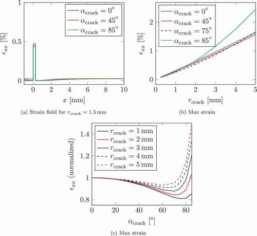
Figure 1. Rail deflection and bending moment due to a train passage. Camera A measures the undeformed rail surface while Camera B measures the deformed surface. The dimensions $L_{\mathrm{w}\mathrm{h}}$, $L_{\mathrm{b}}$, and $L_{\mathrm{w}\mathrm{a}}$ are described in Table 1, and $L_{\mathrm{c}}$ is the distance from the wheel to Camera B.

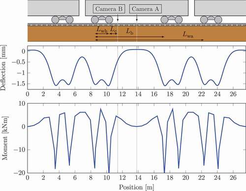
Rails, sleepers and the ground deflects when a train rolls over, as illustrated in Figure 1. These results are calculated for a freight train with a 25-ton axle load using the methodology described in Section 5.1. The rail deflections give rise to bending moments in the rail. Figure 1 shows that the bending moment in the middle of each waggon is approximately zero. Camera A can then take a reference image, showing the rail surface without an applied bending moment. When the train has moved so that Camera B is approximately in Camera A’s previous position, Camera B acquires an image of the same area as Camera A’s reference image. This approximate position is calculated from the train speed. The DIC pattern recognition is then used in an optimization loop to accurately determine the relative position of the images. The image from camera B shows the surface being affected by tensile strains due to a positive rail bending moment. These tensile strains cause the cracks to open, see Figure 2. The crack opening causes a displacement jump over the crack mouth leading to an infinite strain. However, in DIC, the strain is calculated based on displacement between points with a finite spacing. Therefore, the strain illustrated in Figure 2 is not a Dirac delta function. If the point spacing is small enough, a high strain concentration is detected around the crack mouth. This strain concentration is the proposed crack indicator. Finally, we note that the train direction does not matter: the reference image from Camera A can be taken before or after the image from Camera B.

Figure 2. Illustration of the measured strain around a crack mouth in a rail subjected to a positive bending moment.

3. Experimental setup

The initial evaluation of the crack detection method consists of two experimental parts. First, a rail sample is mounted in a test rig, subjected to a bending moment, and analysed using DIC. Second, the crack networks in the examined rail part are characterized by serial sectioning. The investigated field sample was taken from the Swedish mainline (Gothenburg–Stockholm) and has sustained 11 years of traffic, corresponding to approximately 165 MGT. Further details, including the rail’s chemical composition, are given in Meyer et al. [21].

3.1. Crack detection using DIC

Two rail field samples were connected by threaded rods, as shown in Figure 3. Two hydraulically connected cylinders load the samples in 4-point bending. This setup gives a constant bending moment in the part of the rail located between the cylinders. The hydraulic pressure was controlled by a manual pump and measured by an electronic pressure sensor.

Figure 3. DIC experimental setup with the yellow hydraulic cylinders exerting a 4-point bending in the rail samples.

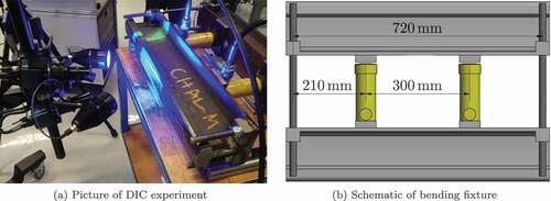
The commercial GOM stereo-DIC system used in this study relies on a speckle pattern to create a 3-dimensional surface. We applied this pattern by first spray-painting the railhead black, followed by spraying white paint at approximately 50% coverage. The surface strains were then measured for the unloaded reference state and at two additional pressure levels, corresponding to bending moments of approximately 7.5 kNm and 15 kNm. Stitching together eight different camera positions (2x4) increased the covered portion of the rail.

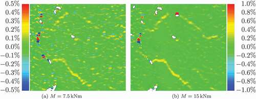
Figure 4 shows that strain concentrations can be observed at a 7.5 kNm bending moment. Increasing the bending moment to 15 kNm improves the Signal to Noise Ratio (SNR) and makes the strain concentrations clearer, see Figure 4(b). The results in Figure 1 only show a 3.8 kNm bending moment. However, this moment can be increased to above 10 kNm following the optimization of train parameters described in Section 5.1.

Figure 4. Surface strain distribution along the rail (horizontal in this figure), measured by DIC.

3.2. Rail sectioning

The proposed crack detection method is based on surface strains. To investigate how this method performs, detailed information about the true crack network is required. To this end, the analysed section of the rail was extracted and characterized using serial sectioning and microscopy, see Figure 5. The extracted sample was surface ground, followed by polishing, in increments of approximately 0.25 mm. From the initial height, $h_0$ in Figures 5(b), 9 mm was taken off starting from the gauge corner. A 1 mm wide, 0.25 mm deep, reference line for positioning was milled on one side. This line is shown in Figure 5(b).

Figure 5. The extracted sample used to characterize the crack networks.

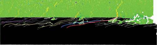
Using a 5X objective lens, resulting in a pixel size of 0.88 µm, 74 mm along the rail was characterized. Multiple image tiles were taken and stitched into one image. For this stitching to work efficiently, a mirror-polished surface is not favourable. For that reason, and from a time-efficiency perspective, grinding marks are still clearly visible in Figure 6. A semi-automated procedure for generating binary images was therefore adopted. Two image layers were created, where the bottom layer contained the raw image. Large dark areas in the bottom layer were filled to become fully black. In the initially transparent top layer, a stylus was used to mark cracks by a 10 pixel (8.8 µm) wide line. After that, we binarized the bottom layer with a threshold of 3 on a 255-level greyscale where 0 is black. Hence, only very dark areas became black. Subsequently, Gaussian filtering (size 20.5 pixels), followed by a binarization (threshold 127), was applied three times to smoothen the image. At this point, the binarized bottom layer contained all large defects that could be identified automatically. As a final step, the top layer, with cracks marked by a stylus, was projected onto the bottom layer.

Figure 6. Example of conversion from optical microscopy images to binary images. The shown images are $1.5\mathrm{m}\mathrm{m}\times 1.5\mathrm{m}\mathrm{m}$.

4. Experimental results

4.1. DIC measurements

The strain field in Figure 7 is visualized for a 15 kNm bending moment. The reference mark, see Figure 5, is on the right side of the strain field. Furthermore, the reference line in Figure 7 shows the horizontal direction in the section images that is along the rail. Hence, it is perpendicular to the reference mark shown in Figure 5(b).

Figure 7. DIC results, viewed from above the microscopy sections. The black rectangle at $x=y=0$ shows the location of the reference mark, and axes correspond to the axes in .Figure 9 with dimensions in mm. The same strain scale as in Figure 4(b) is used. The coloured circles show the end-points of the cracks marked with the corresponding translucent colour in Figure 9

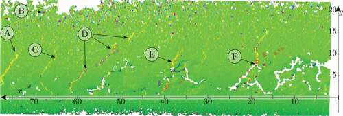
Two types of artefacts are observed in Figure 7. First, the white areas are places where the DIC algorithm was unable to identify the surface. Typically, these artefacts are caused by severe surface irregularities, for example at crack mouths. At reference mark F in Figure 7, the artefact is located in the lower part of the crack mouth, where the geometry is too irregular to be accurately captured by the DIC system. In the upper part, the strain concentration is visible.

The second artefact is the occurrence of red and blue dots. They typically occur in pairs (see e.g. reference mark B). This result implies that high strains of opposite signs are detected close to each other, and the effect cancels out. When these appear just at points and do not coalescence into bands, they can be identified as non-physical artefacts. Two images were taken at each load level when acquiring the DIC results. When comparing these, the red and blue pairs do not remain constant, as opposed to the images’ remaining features. Hence, we conclude that most of these pairs are just random errors stemming from the DIC image processing.

The DIC results provide two relevant sources of information. Firstly, an accurate 3D-map of the rail surface is obtained. This map describes the surface state and the degree of spalling. Secondly, and the primary purpose of the present study, is the strain field due to rail bending. As previously discussed, some strain concentrations continue from regions with high surface irregularities (e.g. at F and E). For the bands denoted by D, several bands almost coalesce into one very long band. At A and C, there are also pronounced bands of high strain concentration. All of these results show the pattern expected based on the simple illustration in Figure 2.

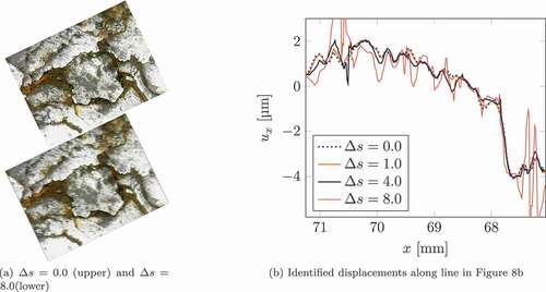
A major drawback with the methodology described so far, is its reliance on a painted speckle pattern. Taken by a simple, low-resolution, USB-microscope, the image in Figure 8(a) shows the rail surface’s natural texture. While the GOM DIC system with the lens used herein gives a 78 pixels/mm resolution, the 640 × 480 USB-microscope’s resolution is $123pixels/mm$. Using this 1.6 times higher resolution enabled subset matching. The open-source software DICe [22] was used to simplify the data processing. While the measured strain field is rather noisy, the displacement field in Figure 8(b) shows a distinct crack (highlighted by the black solid line).

Figure 8. 2D DIC displacement identification based on the natural speckle pattern.

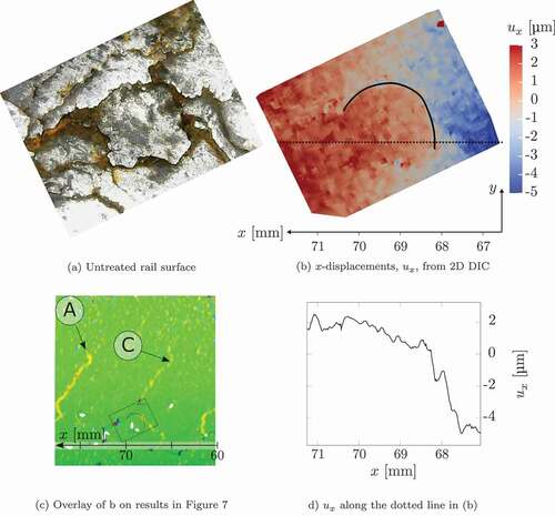
Figure 8(c) shows the location of the 2D-DIC analysis in the 3D-stereo results from Figure 7. The crack indicated in Figure 7 is clear but less severe than some other cracks. To further visualize the displacement jump, Figure 8(d) shows the $x$-displacements jump over the crack mouth. The analysis in Appendix A shows that this 2D-DIC processing also works when considering motion blurring effects. For currently available cameras an analysis speed of 100 km/h is possible considering the motion blurring effect.

4.2. Rail sectioning

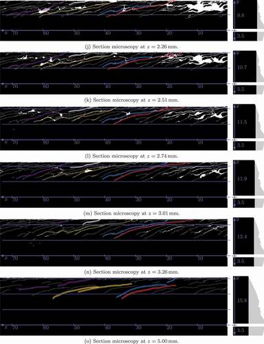
Figure 9 shows microscopy sections with approximately 0.25 mm spacing down to $z=3.26\mathrm{m}\mathrm{m}$, as well as the section at $z=5.00\mathrm{m}\mathrm{m}$. On the right side, the side view of the sectioned part’s profile is shown for clarity. Ground off material is marked with a grey colour. The upwards arrow indicates the approximate distance from the reference line ($y=0$) to the end of the ground surface. The sections in Figure 9 were processed further to improve crack visibility and reduce the manuscript’s file size.¹ The full-sized images are available as a dataset [23]. These binary images also contain sections at 3.75, 4.5, 7.0 and 9.0 mm, which are not included in Figure 9 due to space constraints. Only cracks close to the surface appear in the sections at $z=7.0\mathrm{m}\mathrm{m}$ and $z=9.0\mathrm{m}\mathrm{m}$.

Figure 9. Sections showing the crack patterns with inverted colours compared to Figure 6. All coordinates are in mm. The horizontal lines have 5 mm spacing, the numbers next to the positive and negative y-axes denote the respective axis’ length, and the $z$-coordinate is defined in Figure 5(b). The translucent colours show how different cracks evolve between the sections and their top endpoints are marked by circles of the corresponding colour in Figure 7

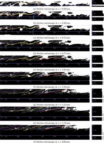
Figure 9. Continued.

The first section, Figure 9(a), was made after a skim pass in the surface grinder and defines $z=0.00\mathrm{m}\mathrm{m}$. Distinct cracks appear as thin white lines against the ground surface appearing black. Depressions due to plastic deformation and material fall-out (spalling) result in larger white areas. Throughout the sections, we will follow five cracks, indicated by purple, yellow, blue, red and white colours. In the supplementary material ‘CracksToDIC_Correlation.pdf’, the sections are put on top of the results in Figure 7 to facilitate interpretation. As an example, the results for $z=-1.51\mathrm{m}\mathrm{m}$ are shown in Figure 10.

Figure 10. Correlation between cracks and DIC surface strains at $z=-1.51\mathrm{m}\mathrm{m}$. More sections are available in the supplementary material ‘CracksToDIC_Correlation.pdf’.

The purple crack breaks the surface at $z=0.00\mathrm{m}\mathrm{m}$ around $x=62\mathrm{m}\mathrm{m}$. Moving down $0.28\mathrm{m}\mathrm{m}$, it extends quite far along the rail ($x$-direction), just under the surface. The crack keeps appearing in roughly the same location, slightly shifting in the positive $y$-direction as the depth increases. Its surface-breaking point also shifts in the positive $y$-direction which is also observed in the DIC results in Figure 7, indicated by the purple circles. The crack appears to be shallow in Figure 9(n). It is marked further into the material as it likely remains connected in the $z$-direction, based on observations in the next section at $z=3.75\mathrm{m}\mathrm{m}$ (only included in supplementary materials). Parts of the crack is also visible in Figure 9(o) ($z=5.00\mathrm{m}\mathrm{m}$), and an approximate crack depth of 1.5 mm can be inferred. Note that the $z$-coordinate does not indicate the crack depth: it is measured perpendicular to the surface (see the profile views on the right in Figure 9.)

The uncertainty in the colour marks are highlighted by the purple crack: the cracks are part of an intricate crack network and it is difficult to tell which cracks are connected between the sections. For example, there is another surface-breaking crack at $x\approx 65\mathrm{m}\mathrm{m}$, that is connected to the purple crack. However, at its surface-breaking point, there are no visible strain concentrations in Figure 7. This crack diminishes after $z=1.24\mathrm{m}\mathrm{m}$, explaining why it doesn’t cause a clear strain concentration. The next surface-breaking crack, around $x=68\mathrm{m}\mathrm{m}$, is also connected to the same network. From around $z=0.77\mathrm{m}\mathrm{m}$, it remains unconnected to the purple network for about 10 mm in the $x$-direction. Consequently, it causes a strain concentration visible around reference marker C in Figure 7.

The yellow crack breaks the surface at $z=0.00\mathrm{m}\mathrm{m}$ around $x=40\mathrm{m}\mathrm{m}$. This point coincides with where the blue and the red crack also break the surface. We will return to these cracks in the next paragraph. Around $x=40\mathrm{m}\mathrm{m}$, $y=4\mathrm{m}\mathrm{m}$ there is a lot of spalling. Consequently, the surface topology is irregular and this can also be observed in the DIC results. At around $y=8\mathrm{m}\mathrm{m}$, at the top of the section at $z=1.73\mathrm{m}\mathrm{m}$, the surface-breaking point of the yellow crack is more distinct. A high strain concentration is measured by the DIC system. Following the yellow crack, it can be seen that it extends very far in the $x$-direction and connects to the purple crack network several centimetres to the left. By using sections between $z=3.26\mathrm{m}\mathrm{m}$ and $z=5.00\mathrm{m}\mathrm{m}$, one can observe that this crack is quite deep, around 3 mm from the surface.

We will now consider the near-surface geometry of the blue crack that also break the surface around $x\approx 40\mathrm{m}\mathrm{m}$ in Figure 9a. From the first 3 sections, the blue crack seems to extend normal to the surface. At its initial surface-breaking point at $x=44.5\mathrm{m}\mathrm{m}$, $y=2.0\mathrm{m}\mathrm{m}$, a slight strain concentration can be observed in Figure 7. Within the first 0.28 mm the crack mouth moves quite a lot to the right, indicating an almost horizontal crack plane, even if the part of the crack around $y=0\mathrm{m}\mathrm{m}$ extends downwards. No clear strain concentration occurs in Figure 7 at the first 5 blue dots. This observation indicates that the DIC results are less sensitive in areas with almost horizontal cracks.

Considering the near-surface geometry of the red crack, a strong strain concentration is observed around its mouth at $x\approx 40\mathrm{m}\mathrm{m}$. Due to the sectioning direction, it is difficult to verify if this result is caused by the red crack or by the larger flake under which the yellow crack seems to pass. The crack morphology is particularly intricate in this area with several long cracks intersecting, in combination with the previously mentioned large spalling. Consequently, it is not possible to determine the depth causing the particular strain concentration at $x\approx 40\mathrm{m}\mathrm{m}$ and $y\approx 4\mathrm{m}\mathrm{m}$ in Figure 7.

The blue and red cracks’ mouths shift far in the negative $x$-direction as we consider deeper sections. In particular, they seem to coalesce into one crack from $z=1.01\mathrm{m}\mathrm{m}$ to $z=3.01\mathrm{m}\mathrm{m}$. At this point, they appear separated again and the red crack seizes to break the surface while the blue remains surface-breaking. For the coalesced sections, only the red crack mouths are marked in Figure 7. We can observe when they again become individual cracks based on the changed strain concentration at reference mark F. As for the yellow crack, the red and blue crack seem, in Figure 9o, to extend some 3 mm below the surface. Still, it is difficult to be certain which cracks they are connected to in that section.

Finally, we will consider the white crack that breaks the surface at $x\approx 53\mathrm{m}\mathrm{m}$. It does not cause a strain concentration in Figure 7, and it is, therefore, important to investigate why. Its markings start in Figure 9d, although it becomes more clear in the later sections. Following this crack until $z=3.26\mathrm{m}\mathrm{m}$, it never extends far into the material: The maximum depth is $0.75\mathrm{m}\mathrm{m}$, and it is reasonable that it is not detected. More surface-breaking cracks than those described above exist. However, the larger cracks surrounding these cracks likely shield the smaller cracks, which reduces the strain concentrations.

5. Numerical evaluation

5.1. Simulation of rail bending

The proposed method relies on the bending moment in the rail caused by the passing measurement train. This initial study only considers slow-moving trains and, therefore, the analyses are quasi-static. The parameters for calculating the bending moments are given in Table 1. Additionally, the code is available as a dataset [24]. The vehicle parameters are from the simulated freight train in Nielsen et al. [25]. We simulate a standard 50E3 rail profile as an Euler-Bernoulli beam, supported by sleepers with 0.65 m spacing via a rail pad. Ballast properties are taken from Li et al. [26], and a representative support width of 0.5 m was chosen for each sleeper, see [24]. Many of these stiffness parameters do not significantly influence the resulting moment, which is of interest in the present study. The main factors influencing the moment distribution are the wheel spacings and the wheel load.

Figure 1 gives the bending moment for a certain position of the train relative to the sleepers. As the train moves forward, the bending moment under the two camera positions changes slightly. This effect is shown in Figure 11a. At Camera A, the moment is rather constant and very close to zero. However, at Camera B, the moment fluctuates when rolling between two sleepers. To maximize the method’s sensitivity for all positions, we must maximize the minimum moment over such a cycle by adjusting the camera position, $L_{\mathrm{c}}$ (see Figure 1 for the definition of $L_{\mathrm{c}}$). Figure 11b shows how the minimum moment varies with camera position. The maximum moment is also included as a reference. The black dot marks the minimum moment at the position of camera B that maximizes the minimum moment. For the parameters in Table 1, this bending moment is 3.8 kNm. The DIC method can calculate the average surface strain and thereby also the bending moment. Hence, a varying bending moment during rolling does not pose an issue for the proposed method. For shallow cracks, there is no discernible difference between a tensile strain for the entire rail or a bending strain in the railhead. Therefore, the method can account for varying complex static and dynamic loading conditions.

Figure 11. Moment variation beneath cameras during rolling. (a) shows the moment variation for the position of Camera B indicated by the black circle in (b).

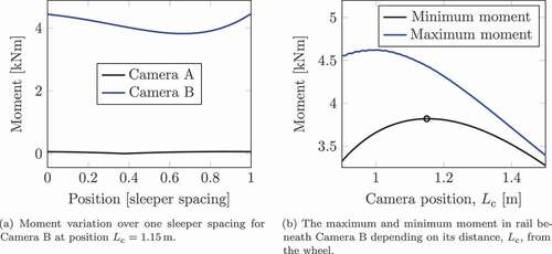
In Section 3.1, we discussed how the Signal-to-Noise-Ratio (SNR) increases with increasing load, illustrated in Figure 4. Therefore, it would be advantageous to increase the bending moment of 3.8 kNm. With the parameters from Table 1, the maximum and minimum rail bending moments are 8.0 kNm and −21.1 kNm respectively. To calculate this, 50 different train positions relative to the sleepers are considered. By adjusting the train’s wheel positions, the bending moment at the camera location can be increased without increasing the load on the rail. Using $L_{\mathrm{w}\mathrm{h}}=1.0\mathrm{m}$, $L_{\mathrm{b}}=8.0\mathrm{m}$, and $L_{\mathrm{w}\mathrm{a}}=14.0\mathrm{m}$, the maximum and minimum rail bending moments become 6.1 kNm and −20.3 kNm respectively. However, the minimum bending moment at Camera B’s position becomes 5.1 kNm.

There are several recommendations for determining the maximum allowable rail bending stress [27]. Most are based on the rail material’s yield strength, ${\sigma }_{\mathrm{y}}$, and give the maximum bending stress, ${\sigma }_{\mathrm{b},\mathrm{m}\mathrm{a}\mathrm{x}}$, as

(1) ${\sigma }_{\mathrm{b},\mathrm{m}\mathrm{a}\mathrm{x}}=\frac{\sigma y-\sigma T}{(1+A)(1+B)(1+C)(1+D)}$(1)

where ${\sigma }_{\mathrm{T}}$ is the thermal stress. The safety factors $A$, $B$, $C$, and $D$ vary. Denoting $s=(1+A)(1+B)(1+C)(1+D)$, the different recommendations in Robnett et al. [27] yield $s\in [1.81,2.14]$. Taking the yield stress for R260 of 534 MPa [28] and assuming a 30°C temperature drop, the conservative maximum bending stress ${\sigma }_{\mathrm{b},\mathrm{m}\mathrm{a}\mathrm{x}}$ becomes 228 MPa. For the rail foot of a 50E3 rail, this corresponds to a bending moment of −49 kNm. Hence, the wheel load can be doubled without violating this limit, if the train is slow enough to neglect dynamic effects . In this case, the minimum bending moment at Camera B’s position becomes 10.2 kNm. In Figure 4, a reasonably good SNR is obtained at 7.5 kNm, hence 10.2 kNm should give a good SNR .

5.2. Finite element modelling of cracks

Figure 7 shows the heterogeneous surface strain caused by cracks. Figure 9 reveals an intricate crack network with a maximum depth of about 3 mm. To better understand the correlation between surface strains and crack morphologies (Figure 12), we use a linear elastic finite element study of a cracked rail subjected to a 15 kNm bending moment (Figure 13). Specifically, we investigate how different crack inclinations, ${\alpha }_{\mathrm{c}\mathrm{r}\mathrm{a}\mathrm{c}\mathrm{k}}$ (Figure 12b), affect the surface strains. Note that the $xyz$-coordinate system here is only approximately equal to the coordinate system used on the field sample. The crack is further parameterized by the crack depth, $r_{\mathrm{c}\mathrm{r}\mathrm{a}\mathrm{c}\mathrm{k}}$. This depth is also the radius of the crack projection onto the $yz$-plane. As shown in Figure 12a, the crack is located in the middle of the gauge corner on the nominal rail profile. Symmetry boundary conditions are applied on the right side sufficiently far from the crack to ensure homogeneous strains at the boundary.

Figure 12. Dimensions of the crack in the finite element model.

Figure 13. Longitudinal strain for a 5 mm deep crack with ${\alpha }_{\mathrm{c}\mathrm{r}\mathrm{a}\mathrm{c}\mathrm{k}}={45}^{\circ }$. Displacements are amplified 50 times.

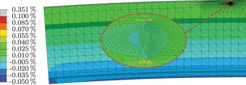
As discussed in conjunction with Figure 2, the DIC method uses the displacement in a discrete set of points to calculate the strain. A facet size of 19 pixels, corresponding to 0.25 mm, was used in the present study. The strains in Figure 14 were calculated from displacements projected onto a grid with 0.25 mm spacing. Hence, these strains can be compared with the strains in Figure 7.

Figure 14. FE-modelling results.

The surface strains at the cracks in Figure 7 are about 0.5%, corresponding to the maximum depth of about 3 mm (Figure 9). The finite element simulation predicts a crack depth of 1.5 mm for 0.5% strain (Figure 14b). Hence, if processing the finite element results as DIC results, strains with the same order of magnitude are found. However, these predictions assume an ideal elliptical crack whose opening is perpendicular to the applied stress. The investigated rail’s crack network is complicated with various angles and interactions between cracks and surface irregularities. Even so, these predictions are useful to understand how the surface strain field can predict the crack severity.

Figure 14a shows the strain along the $x$-axis for three crack angles, ${\alpha }_{\mathrm{c}\mathrm{r}\mathrm{a}\mathrm{c}\mathrm{k}}$, with a crack depth $r_{\mathrm{c}\mathrm{r}\mathrm{a}\mathrm{c}\mathrm{k}}=1.5\mathrm{m}\mathrm{m}$. Due to the numerical approximation of the strain described above, the width of the strain concentration band is 0.25 mm. While the vertical crack has the highest strain concentration at $r_{\mathrm{c}\mathrm{r}\mathrm{a}\mathrm{c}\mathrm{k}}=1.5\mathrm{m}\mathrm{m}$, Figure 14b shows that this trend reverses for deeper cracks with high ${\alpha }_{\mathrm{c}\mathrm{r}\mathrm{a}\mathrm{c}\mathrm{k}}$. The strain concentration increases approximately linear with crack depth, up to a depth of 5 mm and for ${\alpha }_{\mathrm{c}\mathrm{r}\mathrm{a}\mathrm{c}\mathrm{k}}<{75}^{\circ }$. Furthermore, the strain concentration is not strongly dependent on the crack angle. Figure 14c shows this independence: The strain concentration changes less than 20 for ${\alpha }_{\mathrm{c}\mathrm{r}\mathrm{a}\mathrm{c}\mathrm{k}}<{80}^{\circ }$. The strain concentrations for cracks almost parallel to the surface (high angle) are strongly affected by their angle. However, friction, roughness, and non-planar crack surfaces are not considered in the finite element simulations. These features influence such high-angle cracks more than the low-angle cracks. Therefore, a less excessive strain concentration will occur in the field for high-angle cracks.

6. Discussion

The discussion is split into three parts. First, the main findings in the present study are elaborated. Second, solutions to the challenges remaining before the method can be used in the industry are discussed. Finally, possible future enhancements of the method are proposed.

6.1. Main findings

The proposed method utilizes the variation in rail bending stresses inflicted by the measurement train. To assess the feasibility of the proposed method, a simplified quasi-static finite element model is used to obtain the bending moment variation. The exact bending moments in the field are affected by many factors, such as hanging sleepers and dynamic loads. However, the proposed method can determine the variation in bending moment via the average surface strains, and this variation is, therefore, not an issue. Our results show that the quasi-static bending moments can be increased safely by using alternative train configurations. This modification is required for the stereo DIC resolution used in the present work. An alternative is to increase the magnification, as was done for 2D-DIC, to reduce the required bending moment.

The maximum crack depth in our field sample was 3 mm which is similar to other works in the literature: Stock and Pippan [29] produced crack depths around 2 mm in controlled laboratory conditions after ${10}^5$ wheel passages during accelerated testing 23-ton wheel load). For field tests, they found a crack depth of 1.1 mm after 125 MGT in the R260 rail.

This study hypothesizes that the depths of cracks correlate with the surface strain concentration. By tracking the crack network over multiple microscopy sections, we could correlate surface-breaking cracks to the identified strain concentrations. However, the complex crack network of cracks nearly parallel to the surface makes it difficult to establish a clear correlation between each crack and the surface strain concentrations. The strength of the proposed DIC method is that the surface-breaking crack mouths can be individually characterized. Such a high level of detail can provide vital input to research on rail damage. It may also complement traditional techniques, such as ultrasonic and eddy-current. The correlation between crack depth and strain concentration can give early warnings about cracks growing downwards with the potential of causing rail fractures.

6.2. Remaining challenges

6.2.1. Interpretation of results

An efficient condition monitoring system depends on interpretable results that eventually lead to decision making. One advantage of the proposed method is that the results are explicit in terms of individual cracks. This feature is in contrast to other NDT methods that consider so-called indications, cf. A388/A388 M-19 [30]. The more explicit damage detection by the present method can enable differentiation between defects, such as head checks and squats. In this work, an initial study showed the method’s sensitivity to the crack depth. However, more work is required to assess the severity of the damage based on the DIC results. Both numerical studies of different crack morphologies and field studies on various defects should be conducted. Eventually, limit values for various damage types are required for efficient integration in maintenance planning. As the proposed method can characterize the surface profile, results may also be applied to other indices for railway maintenance planning, such as indices developed to estimate the risk of derailment [31].

6.2.2. Design of measurement system

The DIC system must be softly suspended to avoid transferring train vibrations. While the stereo DIC setup is very sensitive to relative motion between the two cameras, much larger motions between the camera setup and the measurement object can be tolerated. Still, the camera positions should adapt to the train motion to capture the rail surface: Firstly, the centre part of each waggon (at Camera A) will move laterally during cornering. Secondly, the camera height must remain fairly constant to maintain image focus. While this is a challenging engineering problem, it seems solvable by using established techniques. Even so, these challenges may limit the maximum speed at which the system can operate. Another engineering challenge is the physical protection of the camera lenses against contamination and damage in snowy and dusty environments. Protection against gravel impacts can be obtained by tight covers having only an opening the size of the field-of-view on top of the rail. Such covers will also limit the influence of changing ambient light conditions. Secondly, an outgoing airflow can prevent dust and water contamination. We stress, however, that designing such a system is not part of the present study.

Without a speckle pattern, a resolution of 123 pixels/mm was used. Measuring a 30 mm wide band thus requires approximately 0.5 megapixels/mm. This pixel density corresponds to 0.5 MB/mm for 8-bit greyscale images. A train moving at 100 km/h will then produce about 14 GB/s per camera. High-performance network communication standards, such as HDR InfiniBand, surpass this requirement by achieving 50 GB/s. Another concern is the data amounts generated. The uncompressed raw data from characterizing a 500 km railway line with four cameras is 1000 TB. Such amounts can be stored by using a sufficient number of drives. However, permanently storing the raw data is not necessary. At the end of a measurement series, the data can be moved to a stationary computer resource for processing, after which only the result must be stored. For example, a damage indicator could be stored with a 1 m resolution. Such data produces 2 MB for 500 km if single-precision floats are used.

6.3. Future developments

The proposed system does not require additional actuators, as in e.g. ultrasonic and eddy-current testing. It is, therefore, suitable for combination with other measurement techniques. For example, surface defects might obscure the large defects that ultrasonic testing should detect. By combining the proposed method with ultrasonic testing, such surface defects may be characterized. Potential risk areas, in which defects may be hidden from the ultrasonic measurements, can then be identified. Furthermore, Rajamäki et al. [7] suggest that eddy-current measurements should be complemented by visual inspection methods. For that purpose, the proposed method could be used as a high-fidelity visual inspection system. Additionally, combining the surface topology with numerical simulations of contact conditions, such as in Li et al. [32], can further improve the damage severity assessment accuracy. Further combinations with railway structural health monitoring (cf [33].) can give accurate load descriptions.

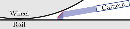
The current study only includes strains due to a positive rail bending moment, compared to a zero moment reference state. This method is the typical application of DIC in crack detection. Most cracks in fatigue loaded samples are perpendicular to the surface and the applied loading direction. Compressive loading will close these cracks. However, typical rail cracks are oriented at an angle when breaking the surface. Therefore, examining the strain field of rails exposed to large negative bending moments could increase the method’s detection capabilities. This measurement can be accomplished by using special lenses as illustrated in Figure 15. Additionally, the crack tip displacements during compressive bending stresses can give further information about the crack opening stress. This will be related to the thermal stress in the rail, potentially giving indications of the risks for sun-kinks during summer and rail fracture during winter.

Figure 15. Custom lens (red) to capture the compressive strains close to the wheel.

7. Concluding remarks

To improve the knowledge of the current rail health status of a railway network, we have proposed a new method for efficient rail crack monitoring. The load from a measurement train induces a strain field on the railhead surface that is measured using Digital Image Correlation (DIC). For bending moments within the safe limits for rail loading, a sufficient signal-to-noise ratio is achieved allowing cracks to be detected.

As opposed to currently used non-destructive tests, the present method can explicitly describe surface-breaking cracks. Supplemented by finite element analyses, we have demonstrated that the method is highly sensitive to crack depth. Using serial sectioning, the 3-dimensional crack networks are characterized and the correlation to the surface strain field is shown. With further research, additional crack characteristics may be identified, such as differentiating between squats and head-checks. Finally, possible strategies for industrial implementations are discussed. In conclusion, the proposed method has the potential to improve rail condition monitoring.

Acknowledgements

This work is part of the activities within the CHARMEC Centre of Excellence at Chalmers University of Technology. Parts of the study have been funded within the Shift2Rail Joint Undertaking in European Union’s Horizon 2020 research and innovation programme in the project In2Track2 and In2Track3 under grant agreements nos. 826255 and 10102456. Our colleague Sebastian Almfeldt at the Architecture and Civil Engineering department kindly lent us their DIC equipment along with his expertise, which was greatly appreciated by the authors.

Disclosure statement

No potential conflict of interest was reported by the author(s).

Supplementary material

Supplemental data for this article can be accessed here

Correction Statement

This article has been republished with minor changes. These changes do not impact the academic content of the article.

Additional information

Funding

This work was supported by the Horizon 2020 Framework Programme [In2Track2, 826255,In2Track3, 10102456].

Notes

1. First, the resolution was decreased by scaling the image down by 80%. Second, it was filtered by a Gaussian filter with size 1 before a threshold of 2 (greyscale 0–255, where 255 is white) was applied. Finally, the resolution was again reduced by 50%.

Appendices

A Motion blur

Subset pattern identification without a speckle pattern succeeded for a $8.13\mu \mathrm{m}$ pixel size. When moving at 100 km/h, it only takes 0.29 s to pass one of these pixels. Hence, very short shutter (exposure) times are necessary to obtain a clear picture for strain identification. To analyze this, we apply a motion blur filter to the images used in Figure 8. The filter is a smoothing filter along the $x$-direction where the contribution to the current pixel is calculated by integrating the fraction of the area covered during the shutter time. We assume a constant velocity motion from position $s_1$ to $s_2$, where $s_{\bullet }$ is measured in pixels. The kernel filter value at position $i$, before normalization, is given by $k_i(\mathrm{\Delta }s)=f_i(-\mathrm{\Delta }s/2)-f_i(\mathrm{\Delta }s/2)$ where $f_i(s)$ is defined as

(2) $f_i(s)=\left\{\begin{array}{cc}0& s\in [-\mathrm{\infty },i-1]\\ 0.5{\left[s-[i-1]\right]}^2& s\in [i-1,i]\\ 1-0.5{\left[i+1-s\right]}^2& s\in [i,i+1]\\ 1& s\in [i+1,\mathrm{\infty }]\end{array}\right.$(2)

This motion blur filter has $i=0$ in the centre and is normalized by ${\sum }_{i=-N}^N{k}_i(\mathrm{\Delta }s)$. For a few examples of $\mathrm{\Delta }s$, the kernels are

(3) $\begin{array}{cc}\mathrm{\Delta }s[\mathrm{p}\mathrm{i}\mathrm{x}\mathrm{e}\mathrm{l}\mathrm{s}]& \mathrm{K}\mathrm{e}\mathrm{r}\mathrm{n}\mathrm{e}\mathrm{l}(1\times 2N+1)\\ 1.0& \left[18,34,18\right]\\ 2.0& \left[14,12,14\right]\\ 4.0& \left[18,14,14,14,18\right]\end{array}$(3)

By applying these filter kernels to raw reference and deformed images like the one in Figure 8a, we simulate a motion blur effect, see Figure 16a. When too much blurring occurs, fewer subsets can be identified in the DIC analysis. Errors are thus introduced in the displacements. Figure 16b shows this effect. In contrast to Figure 8, the image was rotated before the DIC analysis, causing a slightly different result for $\mathrm{\Delta }s=0.0$. Travelling 1 pixel during the exposure time, $\mathrm{\Delta }s=1.0$, has minimal impact on the results. At $\mathrm{\Delta }s=4.0$, the noise increases, but the displacement step around $x=64.7\mathrm{m}\mathrm{m}$ is still distinct. However, for a longer exposure time, $\mathrm{\Delta }s=8.0$, the data noise are at a similar level to the displacement step. In conclusion, an exposure time resulting in 4 pixels traversed provides sufficient measurement accuracy.

From the conducted analysis, a maximum exposure time of 1.16 µs can be accepted. Several commercial high-speed cameras meet this requirement. The remaining challenge is then providing sufficient resolution to cover a wide enough patch of the rail. Providing a $2048\times 1952$ resolution at 3270 fps, the Phantom T1340 camera [34] can cover an approximately 16 mm wide band. Its exposure time is down to 0.5 µs. Hence, based on the above analysis, current commercial cameras appear sufficient for the proposed crack detection system to operate at 100 km/h. Finally, the development of high-speed cameras is rapidly progressing and have not yet approached the theoretical lowest exposure time of 0.024 ns [35]. Future improvements to high-speed imaging can thus reduce the costs and further improve the accuracy and speed of the proposed system.

Figure 16. The motion blur effect.

References

- Heiming M, Candfield J, Lochman L. Track Maintenance & Renewal; 2012. Available from: http://www.cer.be/sites/default/files/publication/2353_7473-11_MARKET_STRATEGY_A4_FINAL.pdf.
- Cannon DF, Edel KO, Grassie SL, et al. Rail defects: an overview. Fatigue Fracture Eng Mater Struct. 2003;26(10):865–886.
- Lidén T, Joborn M. Dimensioning windows for railway infrastructure maintenance: cost efficiency versus traffic impact. J Rail Transp Plann Manage. 2016;6(1):32–47.
- Rowshandel H, Nicholson GL, Davis CL, et al. A robotic approach for NDT of RCF cracks in rails using an ACFM sensor. Insight: Non-Destructive Testing and Condition Monitoring. 2011;53(7):368–376.
- Innotrack. D4.4.1 – rail inspection technologies. : Innotrack; 2008. www.innotrack.eu
- Marais JJ, Mistry KC. Rail integrity management by means of ultrasonic testing. Fatigue Fracture Eng Mater Struct. 2003;26(10):931–938.
- Rajamäki J, Vippola M, Nurmikolu A, et al. Limitations of eddy current inspection in railway rail evaluation. Proc Inst Mech Eng F J Rail Rapid Transit. 2018;232(1):121–129.
- Kishore M, Park J, Song S, et al. Characterization of defects on rail surface using eddy current technique. J Mech Sci Technol. 2019;33(9):4209–4215.
- Pohl R, Erhard A, Montag HJ, et al. Ndt techniques for railroad wheel and gauge corner inspection. NDT E Int. 2004;37(2):89–94.
- Gao Y, Tian GY, Li K, et al. Multiple cracks detection and visualization using magnetic flux leakage and eddy current pulsed thermography. Sens Actuators A. 2015;234:269–281.
- Greene RJ. Crack detection in rail using infrared methods. Opt Eng. 2007;46(5):051013.
- Abidin IZ, Tian GY, Wilson J, et al. Quantitative evaluation of angular defects by pulsed eddy current thermography. NDT E Int. 2010;43(7):537–546.
- Zhan Y, Dai X, Yang E, et al. Convolutional neural network for detecting railway fastener defects using a developed 3D laser system. Int J Rail Trans. 2021;9(5):424–444. Available from.
- Safa M, Sabet A, Ghahremani K, et al. Rail corrosion forensics using 3D imaging and finite element analysis. Int J Rail Trans. 2015;3(3):164–178.
- Deutschl E, Gasser C, Niel A, et al. Defect detection on rail surfaces by a vision based system. In: IEEE Intelligent Vehicles Symposium, 2004, Parma, Italy; IEEE; 2004. p. 507–511.
- Vijaykumar VR, Sangamithirai S. Rail defect detection using Gabor filters with texture analysis. 2015 3rd International Conference on Signal Processing, Communication and Networking, ICSCN 2015, Chennai, India. 2015:6–11.
- Zhuang L, Wang L, Zhang Z, et al. Automated vision inspection of rail surface cracks: a double-layer data-driven framework. Transp Res Part C Emerging Technol. 2018;92(May):258–277.
- Lee JS, Hwang SH, Choi IY, et al. Estimation of crack width based on shape-sensitive kernels and semantic segmentation. Struct Control Health Monit. 2020;27(4):1–21.
- Mohan A, Poobal S. Crack detection using image processing: a critical review and analysis. Alexandria Eng J. 2018;57(2):787–798.
- Jessop C, Ahlström J, Persson C, et al. Damage evolution around white etching layer during uniaxial loading. Fatigue Fracture Eng Mater Struct. 2020;43(1):201–208.
- Meyer KA, Nikas D, Ahlström J. Microstructure and mechanical properties of the running band in a pearlitic rail steel: comparison between biaxially deformed steel and field samples. Wear. 2018;396-397:12–21.
- Turner D. Digital image correlation engine (dice). Sandia Report, SAND2015-10606 O; 2015.
- Meyer KA, Gren D. Rail crack microscopy sections. Available from. 2021; DOI:10.17632/h56kbg2h52.1
- Meyer KA. A simple model to calculate rail bending. Available from. 2021; DOI:10.17632/h355wmc5cf.1
- Nielsen JCO, Kabo E, Ekberg A. Alarm limits for wheel–rail impact loads – part 1: rail bending moments generated by wheel flats. Gothenburg: Chalmers University of Technology; 2009. Available from: https://research.chalmers.se/en/publication/107339.
- Li X, Nielsen JC, Torstensson PT. Simulation of wheel–rail impact load and sleeper–ballast contact pressure in railway crossings using a Green’s function approach. J Sound Vib. 2019;463:1–16.
- Robnett QL, Thompson MR, Hay WW, et al. Technical data bases report, Ballast and foundation materials research program, Report no. FRA-OR&D-76-138. Washington, D.C: U.S. Department of Transportation; 1975. Available from: https://railroads.dot. gov/sites/fra.dot.gov/files/fra_net/15881/1975_TECHNICAL%20DATA% 20BASES%20REPORT%20BALLAST%20AND%20FOUNDATION.PDF.
- Meyer KA, Ekh M, Ahlström J. Modeling of kinematic hardening at large biaxial deformations in pearlitic rail steel. Int J Solids Struct. 2018;130-131:122–132.
- Stock R, Pippan R. Rail grade dependent damage behaviour - Characteristics and damage formation hypothesis. Wear. 2014;314(1–2):44–50.
- ASTM International. A388/A388M Standard Practice for Ultrasonic Examination of Steel Forgings; 2019.
- Janatabadi F, Mohammadzadeh S, Nouri M. A robust complementary index for railway maintenance planning based on a probabilistic approach. Int J Rail Trans. 2021;9(4):380–404. Available from.
- Li Z, Zhao X, Dollevoet R. An approach to determine a critical size for rolling contact fatigue initiating from rail surface defects. Int J Rail Trans. 2017;5(1):16–37.
- Kouroussis G, Kinet D, Moeyaert V, et al. Railway structure monitoring solutions using fibre Bragg grating sensors. Int J Rail Trans. 2016;4(3):135–150.
- Phantom t1340 camera [https://www.phantomhighspeed.com/products/cameras/tseries/t1340]; Accessed: 2021August20.
- Etoh TG, Nguyen AQ, Kamakura Y, et al. The theoretical highest frame rate of silicon image sensors. Sensors. 2017;17(3):8–13.