Physical modelling of pressure flushing of sediment using lightweight materials

Abstract

While designing physical hydraulic model tests to investigate the efficiency of pressure flushing, it is most likely that very fine sediments of cohesive nature are required to satisfy the relevant scaling criteria. Cohesive sediments have different physical properties than sand, and a possibility to avoid such scale effects is to use lightweight materials with a specific gravity larger than water but lower than sand as model sediment. This paper addresses this issue by presenting results from laboratory experiments mimicking pressure flushing through a bottom outlet by using different lightweight materials and sand as model sediments. The results consolidate conclusions of previous studies carried out solely with sand and show that lightweight models can be used to predict the length and volume of flushing cones. Empirical relations to predict the length and volume of flushing cones are proposed and validated against a small set of experimental data from a previous study.

Keywords:

• pressure flushing
• reservoir
• flushing cone
• bottom outlet
• physical modelling
• lightweight sediment

1. Introduction

Reservoir sedimentation is a global problem resulting in continuous depletion of storage capacity of reservoirs by 0.5–1% (Schleiss et al. 2016). In the case of reservoirs used for the generation of hydroelectricity, sediments do not only continuously reduce the live storage capacity but may also induce severe damages on hydro-mechanical components. To counter and/or mitigate reservoir sedimentation, various techniques ranging from reduction of sediment yield by watershed management to evacuation of deposited sediments have been proposed and implemented (Annandale et al. 2016; Basson and Rooseboom 1997; Brandt 2000; Morris and Fan 2010; Schleiss et al. 2016; Wen Shen 1999). Among these techniques, hydraulic flushing is a common worldwide strategy (Lai and Shen 1996) for restoring reservoir storage capacity. In fact, past experiences have shown that flushing is an effective technique to remove sediment deposits in small reservoirs (storage capacity <100 × 10⁶ m³) as well as in large-scale reservoirs (storage capacity up to 10,000 × 10⁶ m³) (Paul and Dhillon 1988).

Pressure flushing removes sediment deposits through bottom outlets, while the reservoir water level is maintained not to be lower than the minimum operating level. Compared to free-flow flushing, in which the reservoir water level is drawn down completely, pressure flushing is less efficient and only scours sediment deposits in the vicinity of bottom outlets by creating a funnel-shaped crater commonly designated as the flushing cone or flushing half-cone (Emamgholizadeh et al. 2006; Mahmood 1987; Meshkati et al. 2010; Wen Shen 1999). A simplified sketch of a flushing cone and associated parameters is shown in Figure 1. Despite its spatially limited extent, pressure flushing is crucial for hydropower reservoirs when sediment deposition levels near intakes have to be controlled to prevent the passage of sand through the turbines while the hydropower plant is in operation (Basson and Rooseboom 2007; Fang and Cao 1996). Moreover, it can be the only feasible option for reservoirs in water-scarce regions, which cannot afford emptying the reservoir for free-flow flushing (Emamgholizadeh et al. 2006; Kondolf et al. 2014; Meshkati et al. 2010).

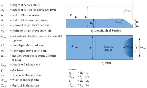
Figure 1. Sketch of a flushing cone and its associated parameters.

Several experimental studies have been carried out to improve the understanding of the processes governing pressure flushing and to address the effect of various hydraulic and sediment parameters on the formation of scour cones. The results from previous studies had established that as soon as the gate of the bottom outlet is opened for pressure flushing, a scour is initiated due to excess shear stress (Powell 2007; Powell and Khan 2012). Large amounts of sediment are released in this first phase, resulting in the formation of the scour cone (Fang and Cao 1996). After the scour cone formation, vortices with vertical axes occur randomly and govern the equilibrium size of the flushing cone by entraining further deposited sediment particles into the flow so that they are flushed through the outlet (Powell 2007; Powell and Khan 2012). With progressing time, the scour cone becomes stable in shape and size with no further sediment removal from the cone (Di Silvio 1990). At this stage, the flushing cone is assumed to achieve an equilibrium for the given hydraulic conditions.

The flushing process can be continued further by drawing down the reservoir water level (Scheuerlein et al. 2004). For a constant outlet discharge, the flushing cone volume increases with a decrease in reservoir water level (Emamgholizadeh et al. 2006; Meshkati et al. 2010). On the other hand, for a constant reservoir water level, an increase in the outlet discharge will further increase the flushing cone volume (Emamgholizadeh et al. 2006; Meshkati et al. 2010). Moreover, it had been found that for a constant outlet discharge (which was regulated in the corresponding experiments) and reservoir water level, the flushing cone increases with an increase in the size of the bottom outlet (Meshkati et al. 2010). However, the flushing cone size not only depends on the opening area of the outlet, but also on its shape. For the outlets with the equivalent opening area, square outlets produce bigger flushing cones than circular outlets (Dreyer and Basson 2018; Hajikandi et al. 2018) but smaller flushing cones than flat rectangular outlets (Dreyer and Basson 2018). For an outlet of specific shape and size, the maximum flushing efficiency can be achieved by flushing at the lowest operational reservoir level, while the bottom outlets are fully opened (Emamgholizadeh et al. 2006; Meshkati et al. 2010).

Besides hydraulic parameters, the size of the flushing cone also depends on sediment properties like the characteristic particle size d_s and thickness of sediment deposit above the outlet’s sill level h_s. The size of the flushing cone increases with decreasing d_s of non-cohesive sediment since finer sediments have a lower angle of repose and are subjected to higher buoyant forces (Fathi-Moghadam et al. 2010). The flushing cone size also increases with increasing h_s due to the additional availability of sediment to be flushed. According to a sensitivity analysis by Emamgholizadeh et al. (2013), the net sediment height above the mid-height of outlet opening H_snet, the characteristic sediment size d_s, the outlet opening diameter D, the average velocity at the outlet u and the net flow depth above the mid-height of outlet opening H_wnet are the most significant parameters regarding the flushing cone dimension and volume. Here, these parameters have been listed in descending order of their significance which means that the sediment properties H_snet and d_s affect the flushing cone geometry more than the hydraulic parameters u and H_wnet.

Although the effect of different hydraulic and sediment parameters on the final geometry of flushing cones was shown experimentally by various authors, it is still difficult to analytically predict the combined effect of all parameters since pressure flushing is a complex three-dimensional phenomenon (Scheuerlein et al. 2004). Therefore, different empirical relationships (Table 1) have been developed by various researchers to predict the flushing cone’s dimensions and volume in a dimensionless framework. However, these empirical relationships provide partly contrasting results. For example, Emamgholizadeh et al. (2013) and Karmacharya et al. (2019) compared the predictions for the scour cone volume based on Equations (4.1) and (5.1) (Table 1) and showed that the corresponding results were significantly different. This can be explained by the fact that the experiments by Meshkati et al. (2010) were carried out with constant values of specific gravity of sediment particles G_s, characteristics sediment size d_s and thickness of sediment deposit H_s, whereas the experiments by Fathi-Moghadam et al. (2010) were performed with constant values of G_s, D and H_s. Therefore, Equations (4.1) and (5.1) may not able to predict the effect of variation in the parameters that were kept constant in the respective experiments.

Table 1. Empirical equations to predict volume and length of a flushing cone

Reference	Empirical equations	Eq. no.
Emamgholizadeh et al. (2006)	${\displaystyle \frac{V_{\text{s}}^{1/3}}{H_{\text{s,net}}}}=0.6139{\left({\displaystyle \frac{u}{\sqrt{g{H}_{\text{w,net}}}}}\right)}^{0.0062}{\left({\displaystyle \frac{H_{\text{s,net}}}{d_{\text{s}}}}\right)}^{0.05}{\left({\displaystyle \frac{H_{\text{s,net}}}{H_{\text{w,net}}}}\right)}^{0.0036}$	1
	where g is the acceleration due to gravity
Powell (2007)	$Z_{\text{max}}={\displaystyle \frac{18576{\displaystyle \frac{H_{\text{wnet}}}{D}}+33273}{{\displaystyle \frac{\rho u}{\mu }}{\left({\displaystyle \frac{d_{\text{s}}}{H_{\text{wnet}}}}\right)}^{0.1}}}$	2.1
	${\displaystyle \frac{W_{\text{max}}}{2}}={\displaystyle \frac{55789{\displaystyle \frac{H_{\text{wnet}}}{D}}+144557}{{\displaystyle \frac{\rho u}{\mu }}{\left({\displaystyle \frac{d_{\text{s}}}{H_{\text{wnet}}}}\right)}^{0.1}}}$	2.2
	$L_{\text{max}}={\displaystyle \frac{72017{\displaystyle \frac{H_{\text{wnet}}}{D}}+45656}{{\displaystyle \frac{\rho u}{\mu }}{\left({\displaystyle \frac{d_s}{H_{\text{wnet}}}}\right)}^{0.1}}}$	2.3
	$V_{\text{s}}=0.673L_{\text{max}}{\displaystyle \frac{W_{\text{max}}}{2}}{Z}_{\text{max}}$	2.4
Shahmirzadi et al. (2010)	${\displaystyle \frac{V_{\text{s}}}{H_{\text{w,net}}^3}}=0.042{\left({\displaystyle \frac{u}{\sqrt{g{H}_{\text{w,net}}}}}\right)}^{0.149}{\left({\displaystyle \frac{H_{\text{s,net}}}{H_{\text{w,net}}}}\right)}^{3.082}{\left({\displaystyle \frac{A}{H_{\text{w,net}}^2}}\right)}^{0.174}$	3.1
		3.2
	${\displaystyle \frac{L_{\text{max}}}{H_{\text{w,net}}}}=0.031{\left({\displaystyle \frac{u}{\sqrt{g{H}_{\text{w,net}}}}}\right)}^{0.104}{\left({\displaystyle \frac{H_{\text{s,net}}}{H_{\text{w,net}}}}\right)}^{0.733}{\left({\displaystyle \frac{A}{H_{\text{w,net}}^{\text{2}}}}\right)}^{0.146}$
	where A is the opening area of the bottom outlet
Meshkati et al. (2010)	${\displaystyle \frac{V_{\text{s}}}{H_{\text{w,net}}^{\text{3}}}}=4.6{\left({\displaystyle \frac{u}{\sqrt{g\left(G_{\text{s}}-1\right)d_{\text{s}}}}}\right)}^{0.21}{\left({\displaystyle \frac{H_{\text{s,net}}}{H_{\text{w,net}}}}\right)}^{2.2}{\left({\displaystyle \frac{D}{H_{\text{w,net}}}}\right)}^{0.89}$	4.1
		4.2
	${\displaystyle \frac{L_{\text{max}}}{H_{\text{w,net}}}}=0.02{\left({\displaystyle \frac{u}{\sqrt{g\left(G_{\text{s}}-1\right)d_{\text{s}}}}}\right)}^{0.1}{\left({\displaystyle \frac{H_{\text{s,net}}}{H_{\text{w,net}}}}\right)}^{0.75}{\left({\displaystyle \frac{D}{H_{\text{w,net}}}}\right)}^{0.34}$
	where Gs is the specific gravity of sediment particles and D is the diameter of outlet’s opening
Fathi-Moghadam et al. (2010)	${\displaystyle \frac{V_{\text{s}}^{1/3}}{D}}=5.28{\left({\displaystyle \frac{u}{\sqrt{g\left(G_{\text{s}}-1\right)d_{\text{s}}}}}\right)}^{0.1}{\left({\displaystyle \frac{H_{\text{w,net}}}{H_{\text{s,net}}}}\right)}^{-0.046}$	5.1
		5.2
	${\displaystyle \frac{L_{\text{max}}}{D}}=8.19{\left({\displaystyle \frac{u}{\sqrt{g\left(G_{\text{s}}-1\right)d_{\text{s}}}}}\right)}^{0.1}{\left({\displaystyle \frac{H_{\text{w,net}}}{H_{\text{s,net}}}}\right)}^{-0.033}$
Dreyer and Basson (2018)	${\displaystyle \frac{L_{\text{max}}}{h_{\text{w}}}}=1.206\text{Ln}\left({\displaystyle \frac{h_{\text{w}}}{h_{\text{w}}-h_{\text{s}}}}\right)-1.4594\text{Ln}\left({\displaystyle \frac{u}{\sqrt{g{h}_{\text{w}}}}}\right)+0.0536\text{Ln}\left({\displaystyle \frac{b_{\text{oc}}+b_{\text{oe}}}{h_{\text{w}}}}\right)$	6.1
		6.2
	${\displaystyle \frac{W_{\text{max}}}{h_{\text{w}}}}=2.3065\text{Ln}\left({\displaystyle \frac{h_{\text{w}}}{h_{\text{w}}-h_{\text{s}}}}\right)-3.4197\text{Ln}\left({\displaystyle \frac{u}{\sqrt{g{h}_{\text{w}}}}}\right)+0.136\text{Ln}\left({\displaystyle \frac{b_{\text{oc}}+b_{\text{oe}}}{h_{\text{w}}}}\right)$
	${\displaystyle \frac{Z_{\text{max}}}{h_{\text{w}}}}=0.7615\text{Ln}\left({\displaystyle \frac{h_{\text{w}}}{h_{\text{w}}-h_{\text{s}}}}\right)-0.7519\text{Ln}\left({\displaystyle \frac{u}{\sqrt{g{h}_{\text{w}}}}}\right)+0.0278\text{Ln}\left({\displaystyle \frac{b_{\text{oc}}+b_{\text{oe}}}{h_{\text{w}}}}\right)$	6.3
	${\displaystyle \frac{V_{\text{s}}}{h_{\text{w}}^3}}={\left({\displaystyle \frac{L_{\text{max}}}{h_{\text{w}}}}\right)}^{1.9529}{\left({\displaystyle \frac{W_{\text{max}}}{h_{\text{w}}}}\right)}^{-0.3787}{\left({\displaystyle \frac{Z_{\text{max}}}{h_{\text{w}}}}\right)}^{1.3663}$	6.4
	where boc is the outlet width over the centreline and boe is the outlet width at the edge

This study evaluates the predictions of those available empirical relations on our experimental data and proposes new empirical relations based on the experimental data. Laboratory experiments were conducted on pressurised flushing of non-cohesive sediment deposit through a bottom outlet by using model sediments of different specific gravities. The objective of this study is to assess the applicability of properly scaled lightweight materials, having a specific gravity lower than sand but higher than water, as model sediment in physical hydraulic modelling specifically in predicting flushing cone geometry. The scaling conditions adopted for selecting model sediments are described in Section 2. Section 2 also describes the experimental setup and procedure for the study. The results of the experiments are presented and discussed in Section 3 in which also new empirical relationships are derived. Section 4 concludes the paper and makes recommendations for future studies.

2. Method

2.1. Experimental setup

Experiments were carried out at the hydraulic laboratory of Norwegian Institute of Science and Technology (NTNU) in Trondheim, Norway, and the hydraulic laboratory of Hydro Lab in Lalitpur, Nepal. The experimental setups at both laboratories were constructed to be hydraulically identical, so that the results are directly comparable. The experimental setup consisted of an inlet tank, a 6 m long, 0.6 m wide and 0.75 m high horizontal flume, and an outlet tank. The inlet tank was connected to the laboratory’s water storage reservoir via a pump and supply pipe. A box with calibrated V-notch was installed at the end of the supply pipe to measure the discharge fed into the inlet tank. At the downstream end, the flume was equipped with a 5 cm × 5 cm orifice at the centreline representing a sluice gate, i.e. a bottom outlet. The sill level of the orifice was kept 6 cm above the flume bed (i.e. a₀ = 6 cm) to allow the free formation of the flushing cone and to avoid the influence of the downstream flow. The opening height of the orifice could be varied from 0 to 5 cm by a vertical slide gate. An outlet tank was installed at the downstream end of the flume to settle the flushed sediment before the outlet discharge was finally released back to the water storage reservoir.

2.2. Model sediments

In total, five sets of experiments were carried out with five different model sediments (Table 2). The model sediments designated as LW-1, LW-2 and LW-3 were lightweight materials and the ones designated as Sand-1 and Sand-2 represented sand. Theoretically, properly scaled lightweight materials can be used in scale models to represent fine sand in the prototype situation, which otherwise would have to be modelled by silt or clay, i.e. by cohesive sediment, hence producing erroneous results due to contrasting sediment properties. Each of the three lightweight sediments had cylindrical grains with a uniform grain size distribution. For the experiments carried out with Sand-1 and Sand-2, poorly graded sands were used keeping the characteristics particle size d₅₀ as close as possible to that estimated by the adopted scaling criteria. The particle size distribution (PSD) curves of selected model sediments are presented in Figure 2. The sorting coefficient C_s from the PSD curves of the Sand-1 and Sand-2 sediments were estimated according to Folk and Ward (1957) to be 0.174 and 0.202, respectively (Table 2). According to the classification scheme by Folk and Ward (1957), sand with C_s< 0.35 is very well sorted. Similarly, the uniformity coefficient C_u for both Sand-1 and Sand-2 were below 6, hence both can be considered as poorly graded sand. Therefore, both Sand-1 and Sand-2 can be considered as very well sorted. The average angle of repose for all the model sediments used in this study including lightweight sediments was ∼35° in dry condition.

Figure 2 PSD of selected model sediments.

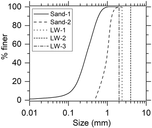
Table 2. Sediments used for the experiments and their properties

Exp. set no.	Sediment material ID	Name of material	Size (ds) mm	Specific gravity (Gs)	Geometric mean size (dg)	Geometric standard deviation $\left({\sigma }_{\text{g}}\right)$	Sorting coefficient (Cs)	Uniformity coefficient, Cu= d60/d10
1	LW-1	Poly-methyl methacrylate (PMMA)	2.40	1.180	2.40	1.00	0	1.00
2	Sand-1	Natural sand	0.30	2.650	0.30	1.67	0.174	2.50
3	LW-2	Masterbatch	4.00	1.400	4.00	1.00	0	1.00
4	Sand-2	Natural sand	1.05	2.650	0.93	1.25	0.202	1.76
5	LW-3	Polystyrene	2.00	1.058	2.00	1.00	0	1.00

The characteristic particle size d_s and specific gravity G_s of the selected sediments were chosen in such a way that LW-1 and Sand-1 can be scaled up to a common arbitrary prototype by scaling the Sand-1 model as a ‘Best model’ [as per classification by Kamphuis (1985)] and the LW-1 model as an undistorted ‘Densimetric Froude model’ [as per classification by Kamphuis (1985)]; hereby, it was assumed that both models have the same length scale ratio L_r, where the subscript ‘r’ defines the ratio of prototype and model properties. A similar scaling relation was maintained between LW-2 and Sand-2 by selecting appropriate values of d_s and G_s. LW-3 was not paired with a sand material as the scaling criteria demanded a very fine sand (d_s< 0.07 mm) which is close to the sand–silt boundary and possibly be subjected to cohesion. However, experiments with LW-3 were carried out to achieve additional data for regression analysis.

For Sand models to be designed as a Best model, similarity in Froude number (F_r = 1), densimetric Froude number (F_*r = 1), relative density of sediment (ρ_s /ρ) and relative roughness (h/d_s) need to be maintained between the model and prototype, where ρ_s is the density of sediment, ρ is the density of fluid, i.e. water, and h is the flow depth. The densimetric Froude number, also known as Shield’s number, represents the ratio of the bed shear stress to the submerged weight of a single sediment particle, and is defined as $F_{\ast }=u_{\ast }^2/\left[\left(G_{\text{s}}-1\right)g{d}_{\text{s}}\right]$, where u_* is the shear velocity. For simplification, the unidirectional flow was assumed in the present flume experiments so that the shear velocity can be defined as $u_{\ast }=\sqrt{\left(ghS\right)}$, where S is the energy gradient of the flow. Since the hydraulics inside a scour cone is complicated to be defined mathematically, uniform flow conditions in the straight reach were considered for scaling the model sediments. The similarity criteria for the ‘Best model’ can be achieved by scaling down the required model sediment diameter with the geometric scale L_r and using the same specific gravity as the prototype sediment, i.e. d_sr = L_r and G_sr = 1.

For a densimetric Froude model of the prototype, similarity in Froude number (F_r = 1) is required and the lightweight sediment must be chosen so that similarity in the densimetric Froude number (F_*r = 1) between the model and the prototype is satisfied. Combining the similarity criteria for densimetric Froude models, i.e. F_r = 1 and F_*r = 1, a simplified relation among the scaling parameters can be derived to design the lightweight sediment models: (7) $L_{\text{r}}={\delta }^2(G_{\text{s}}-1{)}_{\text{r}}{d}_{\text{sr}}$(7)

Here, $\delta$ denotes the distortion ratio (ratio of the horizontal length scale factor to vertical length scale factor) which is equal to unity for geometrically undistorted models.

2.3. Experimental procedure

Each of the five sets of experiments consisted of 32 individual tests which were performed under steady flow conditions for a range of different parameter values (Table 3). Additional 32 tests were carried out for H_s= 100 mm with LW-1 and Sand-1 to provide additional data for validation purposes. Hence, in total, 192 tests were performed in this study. The flume width (B = 0.6 m) and orifice width (b = 0.05 m) were kept constant throughout all the tests. At the beginning of each test, the flume was manually filled with a sediment deposit of uniform thickness H_s. Then the inflow discharge was slowly fed into the flume without disturbing the initial sediment deposit, and the water level was allowed to rise. When the desired water level H_wnet was reached, the gate was opened up to the desired opening height a. The water level H_wnet was chosen from the rating curve of the outlet orifice for the selected opening height, so that the outflow discharge Q was equal to the inflow discharge for the selected water level and the orifice opening height. All tests were carried out without sediment feeding into the inlet discharge. When the flushing cone reached the equilibrium state, the bottom outlet was closed and the water inside the flume was drained slowly without disturbing the shape and size of the flushing cone. The flushing cones were assumed to achieve equilibrium when there was no further sediment erosion inside the cones and their geometry remained stable for the given hydraulic conditions. The achievement of the equilibrium condition in each test was determined by visual observation only. Just to be more certain, the tests were continued to run for some time even after reaching the equilibrium condition. Figure 3 shows examples of flushing cones formed with different model sediments.

Figure 3 Flushing cone formed with (a) LW-1, (b) Sand-1, (c) LW-2, (d) Sand-2 and (e) LW-3.

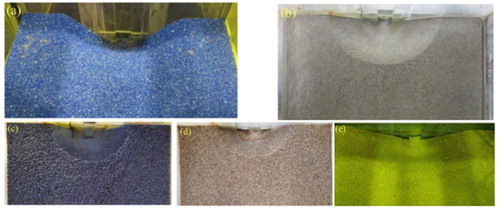
Table 3. Input parameters for 32 tests in each set of experiments

	a	Q	Hwnet	Hsnet		a	Q	Hwnet	Hsnet
Test no.	m	lps	m	m	Test no.	m	lps	m	M
1	0.02	1.3	0.197	0.070	17	0.02	1.3	0.197	0.050
2	0.02	1.7	0.303	0.070	18	0.02	1.7	0.303	0.050
3	0.02	2.0	0.453	0.070	19	0.02	2.0	0.453	0.050
4	0.02	1.8	0.383	0.070	20	0.02	1.8	0.383	0.050
5	0.03	1.8	0.169	0.065	21	0.03	1.8	0.169	0.045
6	0.03	2.2	0.251	0.065	22	0.03	2.2	0.251	0.045
7	0.03	2.6	0.339	0.065	23	0.03	2.6	0.339	0.045
8	0.03	3.0	0.443	0.065	24	0.03	3.0	0.443	0.045
9	0.04	2.5	0.164	0.060	25	0.04	2.5	0.164	0.040
10	0.04	3.2	0.274	0.060	26	0.04	3.2	0.274	0.040
11	0.04	3.9	0.375	0.060	27	0.04	3.9	0.375	0.040
12	0.04	4.3	0.490	0.060	28	0.04	4.3	0.490	0.040
13	0.05	3.2	0.179	0.055	29	0.05	3.2	0.179	0.035
14	0.05	3.8	0.242	0.055	30	0.05	3.8	0.242	0.035
15	0.05	4.7	0.339	0.055	31	0.05	4.7	0.339	0.035
16	0.05	5.0	0.417	0.055	32	0.05	5.0	0.417	0.035

Finally, the surface profile of the flushing cone was measured for each test. For the experimental sets 1 and 5 (Table 2), which were performed at the hydraulic laboratory of NTNU, the surface profiles of the flushing cones were measured using a SeaTek 5 MHz ranging system consisting of 32 acoustic transducers. In the experimental sets 2, 3 and 4, which were carried out at the hydraulic laboratory of Hydro Lab, a point gauge of 1 mm accuracy was used to measure the final flushing cone for each test. The data were used to determine the flushing cone volume with the help of 3D data interpolation function in MATLAB.

3. Results and discussion

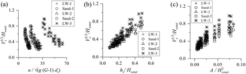
The experimental results were analysed in a dimensionless framework by the following functional relationship that results from a dimensional analysis regarding the flushing cone volume: (8) $\frac{{V_{\text{s}}}^{1/3}}{H_{\text{wnet}}}=f\left(\frac{u}{\sqrt{g\left(G_{\text{s}}-1\right)d_{\text{s}}}},\frac{h_{\text{s}}}{H_{\text{wnet}}},\frac{A}{H_{\text{wnet}}^2}\right)$(8) where $u=Q/A$ and h_s = H_s − a₀. The plots, as shown in Figure 4, of dimensionless flushing cone volume $\left(\frac{{V_{\text{s}}}^{1/3}}{H_{\text{wnet}}}\right)$ against each of $\frac{u}{\sqrt{g\left(G_{\text{s}}-1\right)d_{\text{s}}}}$, $\frac{h_{\text{s}}}{H_{\text{wnet}}}$ and $\frac{A}{H_{\text{wnet}}^2}$ show that the data points for the aforementioned pairs of lightweight sediment and sand are almost overlapping and show a similar trend. Therefore, it can be concluded that the chosen lightweight sediments satisfy the scaling criteria and that they behave similar to sand so that they represent suitable model sediments.

Figure 4 Plots of $\frac{V_s^{1/3}}{H_{wnet}}$ against (a) $\frac{u}{\sqrt{g(G_s-1)d_s}}$, (b) $\frac{h_s}{H_{wnet}}$ and (c) $\frac{A}{H_{wnet}^2}$ for different ‘a’ and $h_s$.

3.1. Flushing cone geometry

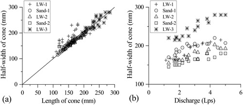
The planform of the final flushing cones after reaching equilibrium conditions was close to a semi-circular shape. The centre of the semi-circular shape was at the middle of the orifice, i.e. the flushing cone width was about twice as long as the length (Figure 5(a)). This result complies with the results obtained by Meshkati et al. (2010), Shahmirzadi et al. (2010), Powell and Khan (2012), Dreyer and Basson (2018) and Sawadogo et al. (2019). It also shows that the flushing cone geometry formed by lightweight sediment is similar to that formed by sand. According to Meshkati et al. (2010) and Powell and Khan (2012), the flushing cone length and width increase with increasing outflow discharge. The overall trend of data points for each model sediment presented in Figure 5(b) shows that the width of flushing cones formed with sand as well as lightweight sediments in the present study was increasing with the increase in outflow discharge and confirms hence these results. A direct comparison of the trends in data points for the tests carried out with Sand-1 and Sand-2 indicates that for the same specific gravity of non-cohesive sediment material, the size of the flushing cone increases as the particle size decreases. This consolidates the conclusions made by Scheuerlein et al. (2004), Fathi-Moghadam et al. (2010) and Powell and Khan (2012). It can also be observed that, in response to changes of the outlet discharge, the overall trend in the width (or length) of the flushing cones formed by lightweight sediment is comparable to the ones formed by sand.

Figure 5 Half-width v/s (a) length of flushing cones, (b) discharge for $H_s=140\mathrm{m}\mathrm{m}$.

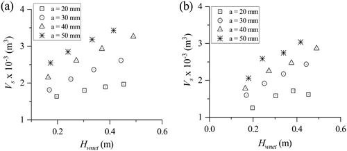
3.2. Flushing cone volume

For a constant orifice area, the flushing cone volume increased with increasing net available head and hence with increasing outlet discharge. Since the geometry of flushing cones formed with lightweight sediments responded to different hydraulic conditions in a similar way as those formed with sand, the plots of lightweight sediments LW-1 and LW-2 for H_s = 140 mm only are presented in Figure 6 for illustration. Figure 6 also shows that the flushing cone volume increases with increasing opening area of the orifice under a constant net head. The results support hence the conclusions made by Emamgholizadeh et al. (2006), Meshkati et al. (2010), Shahmirzadi et al. (2010), Fathi-Moghadam et al. (2010), Dreyer and Basson (2018) and Sawadogo et al. (2019). The results show that the maximum volume of sediment deposit can be flushed when the outlet discharge is the maximum for a given outlet opening. Ideally, the combination of the lowest reservoir level and maximum outlet discharge, which can be achieved by a bigger outlet opening, produces the maximum flushing efficiency. However, providing large outlets in a dam, especially in high head dams, is not always feasible and hence the optimisation of outlet opening size with respect to required minimum reservoir operation level and available discharge for flushing is essential for best results in practice.

Figure 6 Plot of $V_s$ against $H_{wnet}$ for $H_s=140\mathrm{m}\mathrm{m}$ using (a) LW-1 and (b) LW-2.

3.3. Comparison between lightweight sediment and sand

Since the lightweight sediments LW-1 and LW-2 were paired with Sand-1 and Sand-2 sediments, respectively, the results from these tests can be directly compared using scale-invariant dimensionless parameters. Figure 4 shows that the plots of the dimensionless variables for the lightweight sediment and its paired sand extend over the same range under identical test conditions. The dimensionless length $\left(\frac{L_{\text{max}}}{H_{\text{wnet}}}\right)$ and dimensionless volume $\left(\frac{{V_{\text{s}}}^{1/3}}{H_{\text{wnet}}}\right)$ of flushing cones formed with lightweight material and its paired sand are presented in Table 4. For the sand and its paired lightweight models, the dimensionless flushing cone length and volume were in good agreement, as shown in Figure 7(a,b), respectively. Hence, it can be concluded that properly scaled lightweight materials in physical hydraulic models can replicate the pressure flushing of non-cohesive sediment in the prototype. In this study, uniform-sized lightweight materials were used in the model to represent graded sand. Therefore, the results also support the practice of using lightweight materials that are uniformly sized to the required characteristic particle diameter d₅₀ in order to represent graded sand.

Figure 7 Comparison of (a) $\frac{L_{max}}{H_{wnet}}$ and (b) $\frac{V_s^{1/3}}{H_{wnet}}$ for the Sand/Lightweight sediment pairs.

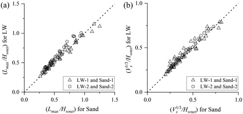
Table 4. Output parameters from 32 tests performed with selected model sediments

	Vs^1/3/Hwnet					L/Hwnet
Test no.	LW-1	Sand-1	LW-2	Sand-2	LW-3	LW-1	Sand-1	LW-2	Sand-2	LW-3
1	0.53	0.62	0.55	0.53	0.72	0.82	0.86	0.76	0.66	1.12
2	0.38	0.41	0.38	0.35	0.48	0.57	0.58	0.54	0.46	0.73
3	0.27	0.28	0.26	0.25	0.33	0.40	0.41	0.35	0.33	0.51
4	0.31	0.32	0.31	0.28	0.39	0.46	0.48	0.42	0.37	0.61
5	0.69	0.78	0.69	0.65	0.88	1.03	1.12	0.95	0.83	1.36
6	0.50	0.53	0.49	0.47	0.62	0.73	0.78	0.68	0.60	0.92
7	0.39	0.40	0.38	0.35	0.47	0.57	0.60	0.50	0.44	0.74
8	0.32	0.31	0.30	0.27	0.37	0.45	0.46	0.43	0.36	0.60
9	0.80	0.81	0.74	0.73	0.98	1.16	1.25	1.01	0.95	1.43
10	0.52	0.49	0.48	0.46	0.62	0.74	0.73	0.69	0.58	0.91
11	0.41	0.37	0.36	0.34	0.47	0.57	0.55	0.52	0.44	0.72
12	0.32	0.29	0.29	0.26	0.38	0.45	0.42	0.42	0.34	0.57
13	0.79	0.77	0.71	0.70	0.97	1.12	1.12	0.92	0.89	1.42
14	0.62	0.57	0.57	0.52	0.74	0.87	0.85	0.79	0.68	1.05
15	0.47	0.42	0.41	0.39	0.55	0.66	0.60	0.59	0.50	0.80
16	0.39	0.35	0.35	0.32	0.45	0.55	0.50	0.48	0.43	0.68
17	0.49	0.54	0.48	0.47	0.59	0.70	0.76	0.69	0.63	0.91
18	0.35	0.36	0.33	0.31	0.41	0.49	0.48	0.46	0.45	0.66
19	0.24	0.25	0.23	0.23	0.29	0.34	0.35	0.33	0.31	0.44
20	0.28	0.29	0.27	0.26	0.34	0.39	0.41	0.38	0.35	0.52
21	0.63	0.64	0.61	0.57	0.77	0.88	0.86	0.86	0.71	1.15
22	0.45	0.45	0.43	0.41	0.54	0.63	0.62	0.60	0.56	0.84
23	0.36	0.34	0.32	0.31	0.42	0.49	0.46	0.46	0.41	0.68
24	0.29	0.26	0.26	0.24	0.33	0.39	0.37	0.38	0.33	0.52
25	0.72	0.67	0.67	0.62	0.85	0.99	0.98	0.95	0.82	1.25
26	0.47	0.42	0.42	0.39	0.54	0.64	0.59	0.57	0.51	0.77
27	0.37	0.32	0.32	0.29	0.41	0.49	0.44	0.40	0.37	0.65
28	0.29	0.24	0.25	0.23	0.33	0.39	0.35	0.34	0.30	0.51
29	0.70	0.64	0.64	0.59	0.85	0.97	0.92	0.92	0.78	1.28
30	0.55	0.47	0.49	0.45	0.65	0.75	0.67	0.68	0.58	0.95
31	0.42	0.36	0.36	0.33	0.49	0.57	0.49	0.50	0.43	0.71
32	0.35	0.30	0.30	0.27	0.40	0.47	0.42	0.42	0.36	0.58

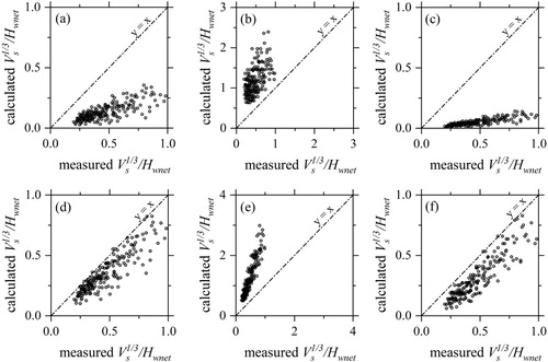
3.4. Comparison of past empirical relations

The performance of past empirical equations to estimate dimensionless flushing cone volume for our experimental data were also evaluated by comparing the measured dimensionless flushing cone volume against that predicted by each of the empirical equations, Equations (1)–(6) as listed in Table 1. Figure 8 shows that the equations proposed by Emamgholizadeh et al. (2006), Shahmirzadi et al. (2010), Meshkati et al. (2010) and Dreyer and Basson (2018) under-estimated the dimensionless volume of the flushing cone, whereas the equations proposed by Powell (2007) and Fathi-Moghadam et al. (2010) over-estimated it. Comparatively, equations proposed by Meshkati et al. (2010) and Dreyer and Basson (2018) made better predictions than others, though the results are under-estimated. The underestimation of the flushing cone volume by Equation (4) could be due to the difference in the shape of the outlets, since Meshkati et al. (2010) used circular outlets, whereas square and flat rectangular outlets were used in this study. Hajikandi et al. (2018) and Dreyer and Basson (2018) had shown that square and flat rectangular outlets produce bigger flushing cones than the circular one. However, Equation (6) also considers outlet’s shape in terms of b_oc and b_oe but still under-estimated the flushing cone volumes. The possible reason behind the over-estimation of flushing cone volume by empirical equations proposed by Powell (2007) could be that the equations were derived for the constant thickness of sediment deposit with its surface at the level of outlet’s sill, i.e. h_s = 0. It may overestimate the volume while extrapolating for h_s > 0. Fathi-Moghadam et al. (2010) also over-estimated the dimensionless flushing volume which consolidated the conclusion made by Emamgholizadeh et al. (2013). Equations (1), (2), (3) and (5) seem to be unsuitable for the range of parameters used in this study. Since the available empirical relations did not fit well in our data, new regression-based empirical relations were derived to predict dimensionless volume and length of flushing cones.

Figure 8 Comparison of measured dimensionless volume $V_s^{1/3}/H_{wnet}$ against that predicted using empirical equations proposed by (a) Emamgholizadeh et al. (2006), (b) Powell (2007), (c) Shahmirzadi et al. (2010), (d) Meshkati et al. (2010), (e) Fathi-Moghadam et al. (2010) and (f) Dreyer & Basson (2018).

3.5. Regression analysis

Out of 160 experimental data points for all 5 model sediments with H_s = 120 and 140 mm, 120 data points were randomly selected as the training data set for regression analysis. The remaining 40 data points were combined with the additional 32 data points (16 from each of LW-1 and Sand-1 model tests with H_s = 100 mm) and used as the testing data set for validation of the regression model. Based on the functional relationship given by Equation (8), multi-variate non-linear regression analyses were carried out and Equations (9) and (10) were derived to predict the dimensionless flushing cone volume and length, respectively (9) $\begin{array}{rl}\frac{{V_{\text{s}}}^{1/3}}{H_{\text{wnet}}}& =1.173{\left(\frac{u}{\sqrt{g\left(G_{\text{s}}-1\right)d_{\text{s}}}}\right)}^{0.203}\\ & \times {\left(\frac{h_{\text{s}}}{H_{\text{wnet}}}\right)}^{0.522}{\left(\frac{A}{H_{\text{wnet}}^2}\right)}^{0.221}\end{array}$(9) (10) $\begin{array}{rl}\frac{L_{\text{max}}}{H_{\text{wnet}}}& =1.311{\left(\frac{u}{\sqrt{g\left(G_{\text{s}}-1\right)d_{\text{s}}}}\right)}^{0.286}\\ & \times {\left(\frac{h_{\text{s}}}{H_{\text{wnet}}}\right)}^{0.588}{\left(\frac{A}{H_{\text{wnet}}^2}\right)}^{0.203}\end{array}$(10)

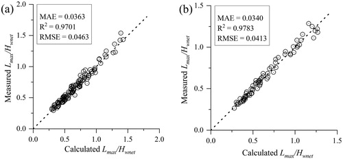
Figure 9(a,b) shows the plots of measured $\frac{{V_{\text{s}}}^{1/3}}{H_{\text{wnet}}}$ against $\frac{{V_{\text{s}}}^{1/3}}{H_{\text{wnet}}}$ estimated by Equation (9) for training and testing datasets, respectively. In the same way, Figure 10(a,b) shows the plots of measured $\frac{L_{\text{max}}}{H_{\text{wnet}}}$ against $\frac{L_{\text{max}}}{H_{\text{wnet}}}$ estimated by Equation (10) for training and testing datasets, respectively. The statistics regarding validation of Equations (9) and 10 (Figures 9(b) and 10(b), respectively) show that the proposed equations provide good predictions even when the testing dataset also includes H_s = 100 mm data, while the training data only account for H_s = 120 and 140 mm.

Figure 9 Plot of measured $\frac{V_s^{1/3}}{H_{wnet}}$ against estimated $\frac{V_s^{1/3}}{H_{wnet}}$ for (a) training dataset and (b) testing dataset.

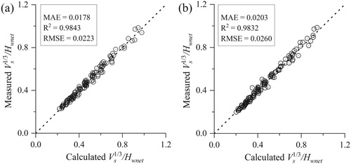
Figure 10 Plot of measured $\frac{L_{max}}{H_{wnet}}$ against estimated $\frac{L_{max}}{H_{wnet}}$ for (a) training dataset and (b) testing dataset.

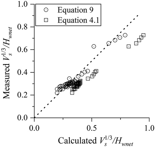
To further test Equation (9), 45 experimental data from Fathi-Moghadam et al. (2010) were extracted and used to predict the dimensionless flushing cone volume (Figure 11). Moreover, the dimensionless flushing cone volume was also predicted using the empirical equations proposed by Meshkati et al. (2010). Figure 12 shows the comparison of measured $\frac{{V_{\text{s}}}^{1/3}}{H_{\text{wnet}}}$ values against the predictions made by Equations (9) and (4.1). The figure shows that estimations of $\frac{{V_{\text{s}}}^{1/3}}{H_{\text{wnet}}}$ by Equation (9) for the data from Fathi-Moghadam et al. (2010) are more accurate than those by Equation (4.1). As mentioned before, Meshkati et al. (2010) carried out experiments with constant H_snet, G_s and d_s and varied A, whereas Fathi-Moghadam et al. (2010) performed experiments with constant H_snet, G_s and A and varied d_s. Hence, Equation (4.1) might be unable to predict the variation in $\frac{{V_{\text{s}}}^{1/3}}{H_{\text{wnet}}}$ due to changes in d_s and H_snet values. However, in this study, experiments were carried out with varying H_snet, G_s, d_s and A (Table 3), and therefore, Equation (9) is able to predict $\frac{{V_{\text{s}}}^{1/3}}{H_{\text{wnet}}}$ for variation in all these parameters.

Figure 11 Prediction of $\frac{V_s^{1/3}}{H_{wnet}}$ for Fathi-Moghadam et al. (2010) experimental data using Eq. 9.

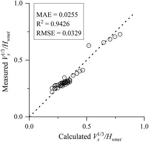
Figure 12 Prediction of $\frac{V_s^{1/3}}{H_{wnet}}$ for Fathi-Moghadam et al. (2010) experimental data using Eq. 4.1 and Eq. 9.

4. Conclusions and recommendations

An experimental investigation of pressure flushing of non-cohesive sediment deposits through a bottom outlet was carried out by using three lightweight materials and two sand materials as model sediments. Two lightweight materials LW-1 and LW-2 were paired with sand material Sand-1 and Sand-2, respectively. The lightweight sediment and sand from each pair were selected in such a way that they can be scaled up to a common arbitrary prototype by scaling the Sand-1 model as a ‘Best Model’ and the LW-1 model as an undistorted ‘densimetric Froude model’.

The experimental results consolidated the conclusions made by previous authors on the geometry of the flushing cones. The plan of flushing cones is close to semi-circular in shape and has its centre at the middle of the outlet’s opening width. The experimental results for lightweight sediment satisfied the functional relationship of dimensionless variables, thus to confirm that the lightweight sediment can mimic the processes of natural sediment. The trends in dimensionless variables for lightweight sediment and its paired sand were comparable. The dimensionless flushing cone length and volume for lightweight sediments are close to those for the respective natural sand in each pairing. Thus, it can be concluded that properly designed densimetric Froude models with lightweight sediments can be used to fairly replicate prototypes with very fine sand, specifically in the case of pressure flushing of non-cohesive sediment deposit through bottom outlets. As per the experimental results, it can be added that uniform-sized lightweight materials can be used in physical hydraulic models to represent graded sand in the prototype. Finally, regression-based empirical equations to predict the length and volume of the flushing cone were proposed. However, the range of variables in this study was constrained by the capacity of laboratory facilities and hence the proposed equations might not be viable for significantly different range of variables.

It should be noted that the average angle of repose for the selected model sediments was approximately close to each other (about 35°) when measured in the dry state. The angle of repose is a significant parameter to determine the final geometry of flushing cones. The replication of flushing cone experiments with sand by using lightweight materials having a significantly different angle of repose may produce different results. Hence, further study in future is recommended using lightweight materials having a different angle of repose. In this study, both sand and lightweight materials were treated as model sediments which satisfy the selected scaling criteria. Future studies with lightweight material as model sediment and sand as prototype sediment by using scaled-up experimental setup for sand model are recommended to quantify the scale effects. The validation of the proposed empirical relation against existing reservoir data as far as possible is also recommended for further study. This study does not cover time scaling in physical hydraulic models. Mobile bed models have different time scales for hydrodynamics and sediment motion. Further studies on time scaling are recommended specially for unsteady flow conditions.

Nomenclature

a	=	opening height of the bottom outlet
a0	=	height of the bottom sill above the flume bed
A	=	cross-sectional area of the orifice
b	=	opening width of the bottom outlet
boc	=	outlet width over the centreline
boe	=	outlet width at the edge
B	=	width of the flume
ds	=	characteristic sediment particle size
D	=	diameter of the circular bottom outlet
g	=	acceleration due to gravity
Gs	=	specific gravity of sediment particles
hs	=	sediment height above outlet’s sill
Hs	=	sediment height above the flume bed
Hsnet	=	net sediment height above the centre of the outlet opening
hw	=	flow depth above outlet’s sill
Hw	=	flow depth above flume bed
Hwnet	=	net flow depth above the centre of the outlet opening
Lmax	=	length of the flushing cone at equilibrium
Q	=	discharge
u	=	average flow velocity at the orifice
Vs	=	equilibrium volume of the flushing cone
Wmax	=	width of the flushing cone at equilibrium
Zmax	=	depth of the flushing cone at equilibrium

Additional information

Funding

This study was conducted as a joint collaboration between Norwegian Institute of Science and Technology (NTNU), Norway, and Hydro Lab Pvt. Ltd, Nepal, under SediPass programme with funding from The Research Council of Norway.

Notes on contributors

Sanat Kumar Karmacharya

Sanat Kumar Karmacharya is a PhD candidate at Department of Civil and Environmental Engineering from Norwegian University of Science and Technology (NTNU). He has more than 10 years of experience in physical hydraulic model studies, sediment sampling and laboratory analyses and field measurements of hydraulic and sedimentological parameters. His main research interests include hydraulic modelling, sedimentation, hydraulic structures and hydrology.

Nils Ruther

Nils Ruther is a Professor at Department of Civil and Environmental Engineering from Norwegian University of Science and Technology (NTNU). He has over 15 years’ experience in the field of hydraulic and sediment transport engineering His research interests are mainly within the fields of numerical modelling of sediment transport, fluvial hydraulics, environmental river mechanics, basic sediment transport, ecohydraulics and hydraulic structures. He has also been contributing to advancements in measurement technology for sediment transport quantification in fluvial environment.

Jochen Aberle

Jochen Aberle is a Professor at Leichtweiß-Institut für Wasserbau, Technische Universität Braunschweig, Germany, and has also 20% involvement as a Professor at Department of Civil and Environmental Engineering from Norwegian University of Science and Technology (NTNU). His main research includes scale model studies, experimental methods and instrumentation, flow–sediment–vegetation interaction, bed stability and sediment transport, and turbulent flow field over rough surfaces.

Sudhir Man Shrestha

Sudhir Man Shrestha earned a Master’s degree in Hydropower Development from Norwegian University of Science and Technology (NTNU) in 2019. He is interested in scale models, hydraulic structures related to hydropower and sedimentation studies. He was involved in this study as a part of his Master’s thesis.

Meg Bahadur Bishwakarma

Meg Bahadur Bishwakarma is the General Manager of Hydro Lab Pvt Ltd, Nepal. He has above 25 years of experience in planning, design, construction supervision, contract management/administration and the environmental mitigation and monitoring of hydro projects. Last 13 years of his work experience involves hydraulic design, physical hydraulic modelling, intensive research on sediment measurement and cost-effective sediment handling including 5 years part time teaching at the Norwegian University of Science and Technology (NTNU).

References

- Annandale GW, Morris GL, Karki P. 2016. Extending the life of reservoirs: sustainable sediment management for dams and run-of-river hydropower [Internet]. Washington (DC): The World Bank. doi:10.1596/978-1-4648-0838-8.
- Basson GR, Rooseboom A. 1997. Dealing with reservoir sedimentation. Pretoria (South Africa): Water Research Commission.
- Basson GR, Rooseboom A. 2007. Mathematical modeling of sediment transport and deposition in reservoirs (bulletin no 140). Int Comm Large Dams.
- Brandt S. A. 2000. A review of reservoir desiltation. Int J Sediment Res. 15(3):321–342.
- Di Silvio G. 1990. Modeling desiltation of reservoirs by bottom-outlet flushing. In: Shen HW, editor. Movable bed phys models [Internet]. Dordrecht: Springer Netherlands; p. 159–171. doi:10.1007/978-94-009-2081-1_16.
- Dreyer S, Basson G. 2018. Investigation of the shape of low-level outlets at hydropower dams for local pressure flushing of sediments. In: SANCOLD 2018 Sustain Dam Eng Ever-Chang World. Cape Town, South Africa.
- Emamgholizadeh S, Bateni SM, Jeng D-S. 2013. Artificial intelligence-based estimation of flushing half-cone geometry. Eng Appl Artif Intell. 26:2551–2558.
- Emamgholizadeh S, Bina M, Fathi-moghadam M, Ghomeyshi M. 2006. Investigation and evaluation of the pressure flushing through storage reservoir. ARPN J Eng Appl Sci. 1(4):7–16.
- Fang D, Cao S. 1996. An experimental study on scour funnel in front of a sediment flushing outlet of a reservoir. In: Proc 6th Fed Interag Sediment Conf. Las Vegas; p. I.78–I.84.
- Fathi-Moghadam M, Emamgholizadeh S, Bina M, Ghomeshi M. 2010. Physical modelling of pressure flushing for desilting of non-cohesive sediment. J Hydraul Res. 48:509–514.
- Folk RL, Ward WC. 1957. Brazos river bar [Texas]; a study in the significance of grain size parameters. J Sediment Res. 27:3–26.
- Hajikandi H, Vosoughi H, Jamali S. 2018. Comparing the scour upstream of circular and square orifices. Int J Civ Eng. 16:1145–1156.
- Kamphuis JW. 1985. On understanding scale effect in coastal mobile bed models. In: Dalrymple RA, editor. Physical modelling in coastal engineering. Rotterdam (Netherlands): A. A. Balkema; p. 141–162.
- Karmacharya SK, Henry P-Y, Bishwakarma M, Aberle J, Rüther N. 2019. Physical modelling of pressurized flushing of non-cohesive sediment using lightweight material. J Phys: Conf Ser. 1266:012012.
- Kondolf GM, Gao Y, Annandale GW, Morris GL, Jiang E, Zhang J, Cao Y, Carling P, Fu K, Guo Q, et al. 2014. Sustainable sediment management in reservoirs and regulated rivers: experiences from five continents: KONDOLF. Earths Future. 2:256–280.
- Lai J-S, Shen HW. 1996. Flushing sediment through reservoirs. J Hydraul Res. 34:237–255.
- Mahmood K. 1987. Reservoir sedimentation: impact, extent, and mitigation [Internet]. [place unknown]: The World Bank; [cited 2019 Oct 14]. Available from: http://documents.worldbank.org/curated/en/888541468762328736/Reservoir-sedimentation-impact-extent-and-mitigation.
- Meshkati MEM, Dehghani AA, Sumi T, Naser G, Ahadpour A. 2010. Experimental investigation of local half-cone scouring against dam. Proc Int conf fluv hydraul; Braunschweig, Germany, p. 1267–1273.
- Morris GL, Fan J. 2010. Reservoir sedimentation handbook: design and management of dams, reservoirs, and watersheds for sustainable use. New York: McGraw-Hill.
- Paul TC, Dhillon GS. 1988. Sluice dimensioning for desilting reservoirs. Int Water Power Dam Constr. 40:40–44.
- Powell D. 2007. Sediment Transport Upstream of Orifices [PhD Thesis], [Internet]. Clemson (SC): Clemson University. Available from: https://tigerprints.clemson.edu/all_dissertations/140.
- Powell DN, Khan AA. 2012. Scour upstream of a circular orifice under constant head. J Hydraul Res. 50:28–34.
- Sawadogo O, Basson GR, Schneiderbauer S. 2019. Physical and coupled fully three-dimensional numerical modeling of pressurized bottom outlet flushing processes in reservoirs. Int J Sediment Res. 34(5):461–474. https://doi.org/10.1016/j.ijsrc.2019.02.001.
- Scheuerlein H, Tritthart M, Gonzalez FN. 2004. Numerical and physical modelling concerning the removal of sediment deposits from reservoirs. In: Proc Int Conf Hydraul Dams River Struct. Tehran, Iran: CRC Press. https://doi.org/10.1201/b16994.
- Schleiss AJ, Franca MJ, Juez C, Cesare GD. 2016. Reservoir sedimentation. J Hydraul Res. 54:595–614.
- Shahmirzadi MEM, Dehghani AA, Meftahh M, Mosaedi A. 2010. Experimental investigation of pressure flushing technique in reservoir storages. Water Geosci. 1:132–137.
- Wen Shen H. 1999. Flushing sediment through reservoirs. J Hydraul Res. 37:743–757.