Multi-class dynamic traffic assignment with physical queues: intersection-movement-based formulation and paradox

ABSTRACT

This paper proposes an intersection-movement-based variational inequality formulation for the multi-class dynamic traffic assignment (DTA) problem involving physical queues using the concept of approach proportion. An extragradient method that requires only pseudomonotonicity and Lipschitz continuity for convergence is developed to solve the problem. We also present a car–truck interaction paradox, which states that allowing trucks to travel or increasing the truck flow in a network can improve network performance for cars in terms of the total car travel time. Numerical examples are set up to illustrate the importance of considering multiple vehicle types and their interactions in a DTA model, the effects of various parameters on the occurrence of the paradox, and the performance of the solution algorithm.

KEYWORDS:

• Multi-class dynamic traffic assignment
• approach proportion
• variational inequality
• extragradient method
• paradox

1. Introduction

Dynamic traffic assignment (DTA) is an important topic due to its wide applications in transport planning and management (Szeto and Lo 2006). In general, DTA can be classified into the simulation-based approach (e.g. Yagar 1971; Mahmassani, Hu, and Jayakrishnan 1995; Mahut and Florian 2010) and the analytical approach (see Ran and Boyce 1996; Peeta and Ziliaskopoulos 2001; Szeto and Lo 2005; and Szeto and Wong 2012 for comprehensive reviews). The simulation-based approach focuses on enabling practical deployment for realistic networks, its applicability in real-life networks, and its ability to capture traffic dynamics and microscopic driver behaviour such as lane-changing behaviour. However, the solution properties of the corresponding models, such as solution existence and uniqueness, are not guaranteed and cannot be determined in advance.

In contrast, the analytical approach is more suitable for analysing the properties of DTA via various frameworks. These frameworks include the optimisation model (Merchant and Nemhauser 1978a, 1978b; Carey 1987; Carey and Watling 2012), optimal control (Friesz et al. 1989; Ran, Boyce, and LeBlanc 1993; Chow 2009a, 2009b; Ma et al. 2014a, 2014b), variational inequality (Friesz et al. 1993; Ran and Boyce 1996; Chen and Hsueh 1998; Huang and Lam 2002; Lo and Szeto 2002a, 2002b; Szeto and Lo 2004, 2006; Han, Friesz, and Yao 2013c), nonlinear complementarity problem (NCP) (Wie, Tobin, and Carey 2002; Ban et al. 2008), nonlinear equation system (Long et al. 2015b), fixed point problem (Szeto, Jiang, and Sumalee 2011; Meng and Khoo 2012), differential variational inequality (Friesz et al. 2013; Friesz and Meimand 2014), and differential complementarity problem (Ban et al. 2012b) frameworks.

All of the preceding analytical frameworks are formulated as either path-based models (e.g. Friesz et al. 1993; Huang and Lam 2002; Lo and Szeto 2002a, 2002b; Szeto and Lo 2004, 2006; Perakis and Roels 2006; Szeto 2008; Szeto, Jiang, and Sumalee 2011) or link-based models (e.g. Carey 1987; Ran and Boyce 1996; Chen and Hsueh 1998; Wie, Tobin, and Carey 2002; Ban et al. 2008). The merit of path-based models is that the path-related information, such as path flows and sets, can be obtained and imported to dynamic network loading (DNL) models to model flow propagation at merges and diverges and track spillback queues. Nevertheless, a path-based model normally suffers from the computational burden of path enumeration or relies on path-generation heuristics with no guarantee on convergence to handle huge path sets, even for medium networks. Instead, link-based models can avoid these two demerits and thus be applied to large networks. However, link-based models cannot be used to capture realistic traffic dynamics such as queue spillback (in one exception, Ma et al. (2014b) proposed a link-based dynamic user optimal (DUO) model that could capture queue spillback for single-destination cases). If it is not captured, the flow pattern and locations of severe congestion may be estimated incorrectly and the strategy adopted may actually worsen network performance (Lo and Szeto 2004, 2005).

To retain the benefits of both the link- and path-based models, Long et al. (2013, 2015a) developed intersection-movement-based DTA models for general networks with multiple destinations. They formulated the traffic assignment problem in terms of approach proportions, that is, the proportion of traffic on the current link or node that selects a downstream link when leaving an intersection (or a node). This definition requires either two adjacent links or one origin link and one outgoing link to define an intersection movement. This is different from the classical definition, according to which only downstream links are used to define the proportion. An approach-proportion implicitly contains the traveller’s path information, as a path can be deduced by checking the downstream links involved in defining the approach proportions from origin to destination. As a result, this type of model can retain the advantages of both the link- and path-based models. First, as in link-based models, path enumeration and path-set generation can be avoided in the solution procedure for intersection-movement-based models. Second, as in path-based models, the realistic effects of physical queues can be captured in intersection-movement-based models when a physical queue DNL model is adopted, as the approach proportions contain the traveller’s path information. However, compared with link-based models, intersection-movement-based models have more decision variables, as each link flow or demand rate is disaggregated by downstream links (which very often number more than one) to define intersection movements and the corresponding approach proportions.

Most of the preceding models, including the intersection-movement-based DTA models, consider only a single vehicle class. It is important to capture multiple vehicle classes in a DTA model and the interactions between different types of vehicles for several reasons. First, interactions between vehicle classes have been identified as a cause of traffic hysteresis, capacity decreases, and the wide scattering of flow–density relationships in a congested regime (Ngoduy 2010). Second, it is clear that trucks have a great influence on highway capacity, as they travel more slowly than cars and can become moving bottlenecks. Therefore, without considering different vehicle types and their interactions, realistic traffic dynamics and queue spillback cannot be modelled properly and the total system travel time cannot be estimated precisely. Third, many empirical studies have shown that vehicle emissions are closely related to speed and vehicle type; for example, the emissions of trucks are greater than those of cars. Therefore, it is important to capture traffic heterogeneity in estimating total vehicle emissions. Fourth, it is essential to distinguish user classes in the application of class-specific or priority control or when different types of traffic information are available to different user classes (Ngoduy 2010).

This paper develops a multi-class intersection-movement-based DTA model based on the DUO principle and concept of approach proportion. The problem is formulated as a VI problem. The DNL model proposed by Bliemer (2007) is modified and incorporated into the VI formulation. Unlike some single-class DNL models (Ban et al. 2012a; Han, Friesz, and Yao 2013a, 2013b), this DNL model can capture car–truck interactions and allow approach proportions to be used as inputs. An extragradient method that requires only mild assumptions is adopted to solve the problem. Numerical examples are set to illustrate the importance of considering multiple vehicle classes. In addition, a car–truck interaction paradox, which states that allowing trucks to travel in a network or increasing the demand of trucks can improve total car travel time, is proposed, discussed, and examined. The findings have important implications for managing road networks with multiple types of traffic. For example, it is possible to relax road restrictions for trucks or large vehicles so that the total car travel time can be further improved or vice versa. The findings also open up new research directions for traffic management such as road restrictions and priority control for specific vehicle classes. This paper makes two main contributions. First, it proposes a multi-class intersection-movement-based DTA model that considers interactions between different types of vehicles and physical queues. Second, it proposes and examines the paradox associated with the interactions between trucks and cars.

The remainder of this paper proceeds as follows. Section 2 introduces the VI formulation for the intersection-movement-based multi-class DTA problem. It then depicts the DNL model encapsulated for calculating the mapping function in the VI formulation. Section 3 presents the extragradient solution method. Numerical examples are given in Section 4. Finally, Section 5 provides our conclusions and future research directions.

2. Formulation

2.1 Notations

We consider a network with multiple origins and destinations and various classes of vehicles according to vehicle type. The network is formed by nodes and links. To simplify the presentation of the formulation, the network is designed to have the following properties. First, a node in a network can only have one status, that is, an origin, a destination, or an intermediate node. Second, at least two links are required to connect an origin and a destination. Third, there is one dummy link coming out from a destination with an infinite capacity. The first requirement can easily be satisfied by designing the network carefully. The second requirement is always satisfied for large networks. For small networks, this requirement can be satisfied by breaking down each link directly connecting an origin and a destination into a pair of links: one going into an intermediate node, and one coming out from the node. The third requirement aims to avoid developing additional sub-models to deal with flow propagation for the links going into a destination.

The following notations are used throughout this paper.

2.1.1 Sets

M	=	set of vehicle classes.
J	=	set of nodes.
N	=	set of origins, .
D	=	set of destinations, .
T	=	set of continuous time indices for the modelling horizon considered, [0, ].
T′	=	set of discretised time indices.
A	=	set of links.
	=	set of links leaving (entering) node j.

2.1.2 Indices

m,	=	class indices, .
i	=	origin index, .
j,	=	node indices, .
d,	=	destination indices, .
t, t’	=	time indices, , .
a, b,	=	indices of links.
	=	tail (head) node of link a.

2.1.3 Parameters

	=	duration of the modelling horizon.
	=	class m demand rate between origin i and destination d at time t.
	=	passenger car unit (PCU) for class m vehicles.
	=	length of link a.
	=	queue density of a single lane on link a.
	=	number of lanes on link a.
	=	maximum travel speed of class m vehicles on link a.
	=	design capacity of link a.
	=	parameters required for the extragradient method.

2.1.4 Decision variables and functions

	=	flow rate of class m vehicles to destination d entering link a from node j at time t.
	=	flow rate of class m vehicles entering link a at time t and passing through the next link b to destination d.
	=	proportion of class m flow to destination d entering link a from node j at time t.
	=	proportion of class m flow entering link a at time t and passing through the next link b to destination d.
	=	minimum travel time for class m vehicles between node j and destination d departing at time t.
	=	minimum travel time for class m vehicles to destination d entering link a from node j at time t.
	=	minimum travel time for class m vehicles between the tail node of link a and destination d via link b departing at time t.
	=	travel time on link a for class m vehicles entering at time t.
	=	exit time for class m vehicles entering link a at time t.
	=	cumulative inflow of class m vehicles into link a and going to destination d via link b until time t.
	=	cumulative inflow of class m vehicles into link a until time t.
	=	cumulative inflow into link a in terms of PCU until time t.
	=	potential outflow rate of class m vehicles from link a at time t and going to destination d via the next link b.
	=	potential outflow rate of class m vehicles from link a to link b at time t.
	=	actual outflow rate of class m vehicles leaving link a at time t and going to destination d via the next link b.
	=	actual outflow rate of class m vehicles from link a to link b at time t.
	=	cumulative flow of class m vehicles leaving link a and going to destination d via the next link b until time t.
	=	cumulative flow of class m vehicles leaving link a until time t.
	=	cumulative outflow from link a in terms of PCU until time t.
	=	class m flow in the queuing part of link a at time t.
	=	length of the free-moving part on link a at time t.
	=	length of the queuing part on link a at time t.
	=	cumulative queue inflow of class m vehicles into link a until time t and travelling to destination d via the next link b.
	=	cumulative queue inflow of class m vehicles into link a until time t.
	=	cumulative queue inflow into link a in terms of PCU until time t.
	=	inflow capacity of link a at time t.

Similar to the link-node-based DUE models in the literature (e.g. Wie, Tobin, and Carey 2002; Ban et al. 2008), our proposed formulation disaggregates the decision variables and associated functions by destination.

2.2 Intersection-movement-based formulation

For a node that is neither an origin nor a destination, there is at least one incoming link and one outgoing link. An intersection can be described by a pair of incoming and outgoing links. An intersection movement represents flow making through or turning movement at that intersection. A traveller’s departure from an origin can also be viewed as an intersection movement, as the origin can be considered as an intersection and the traveller can select links for entering the network. For an origin, the movement of travellers entering into the network is also described by the origin node and the link selected to enter.

2.2.1 Intersection-movement-based multi-class DUO conditions

Based on the preceding definitions, the proposed multi-class intersection-movement-based DUO conditions can be generalised from those in a study by Long et al. (2013), expressed as (1) and (2)

Equation (1) states that if the flow of class m vehicles entering link a from origin i at time t and going to destination d is positive, then the minimum travel time of these vehicles equals the minimum travel time for the same class of vehicles departing at the same time and travelling between the same origin–destination (OD) pair; otherwise, the minimum travel time of these vehicles at least equals the minimum travel time for the same class of vehicles departing at the same time and travelling between the same OD pair. Equation (2) infers that if the flow of class m vehicles entering link a at time t and passing through the next link b to destination d is positive, then the minimum travel time of these vehicles equals the minimum travel time for the same class of vehicles entering the same link at the same time to the same destination; otherwise, the minimum travel time of these vehicles at least equals the minimum travel time for the same class of vehicles departing at the same time from the tail node of link a through that link to destination d.

Following the traditional user equilibrium traffic assignment literature, we assume that drivers’ route choices depend only on their own travel times. Drivers know their route travel times based on experience. We do not assume that any drivers know the truck percentage on the road or that car drivers know the truck travel times. In our study, the travel times of trucks and cars on a road are functions of traffic flow and mix on it and are determined by the DNL model described later. The DNL captures the effect of truck speed (and hence travel time) and truck percentage on car travel times. In other words, truck percentage and truck travel times are indirectly captured by car travel times, and the latter factor affects the route choices of car drivers. However, truck speed and percentage are not factors that directly affect the route choices of car drivers, nor are they factors considered by car drivers.

The minimum travel times, that is, , , and in (1) and (2), are respectively defined by (3) (4) and (5)

In addition, the definitional and non-negativity constraints are depicted as follows: (6) and (7)

The flow conservation constraints are formulated as (8) and (9)

Equation (8) infers that the flow of class m vehicles entering link a at time t and going to destination d is distributed among the links leaving link a. Equation (9) is the node flow conservation constraint, stating that the demand of class m vehicles generated at origin i at time t is split between the links coming out from origin i.

2.2.2 Intersection-movement-based multi-class VI formulation

The intersection-movement-based multi-class DUO conditions can be represented as the following NCP: (10) (11) (12) (13) (14)

and (15)

It is well known that an NCP can be reformulated into a VI problem when the solution set is non-negative orthant. After taking into account the requirement of flow conservation conditions, the intersection-movement-based multi-class VI problem is to determine such that (16) where * denotes an optimal solution to the VI problem and is the solution space defined by the non-negativity constraints (6) and (7) and conservation constraints (8) and (9).

2.2.3 Approach-proportion-based multi-class VI formulation

The preceding formulation can alternatively be reformulated using the concept of approach proportion. An approach proportion is defined as the proportion of vehicles that select a downstream link to enter after leaving a node or passing through an upstream link. That is, it is defined as the proportion of vehicles coming out from a link or a node to enter the relevant approach or the proportion of vehicles selecting a particular intersection movement. By definition, the approach proportions must satisfy the following conditions: (17) (18) (19)

and (20)

Equations (17) and (18) respectively require that the sum of all of the approach proportions associated with an origin and an intermediate node must equal one. Equations (19) and (20) impose the restriction that all of the approach proportions must be nonnegative.

Approach proportions must also satisfy the following by definitions: (21) and (22)

The approach-based DUO conditions can be expressed as (23) and (24)

It is shown in the Appendix that the approach-based DUO conditions (23) and (24) imply the link-based DUO conditions (1) and (2).

The corresponding VI problem is to determine such that (25) where * denotes an optimal solution and is the solution space of the approach proportions defined by Equations (17)–(20). The mapping function of the VI is defined by , which in turn is a function of , the outputs of a DNL model given .

2.3 DNL model

A DNL model depicts how traffic propagates inside a traffic network and hence governs network performance in terms of travel time. In general, many DNL models can be used (e.g. see Mun 2007). To be more realistic, we modify the model developed by Bliemer (2007), which captures dynamic queuing, spillback effects, and multiple vehicle types. Bliemer’s model is divided into two sub-models: a link model and a node model. The link model describes the flow propagation and outputs queue lengths and queue inflow rates given the inflow rates. The node model determines the actual outflow rate from each link. Afterwards, the inflow rate into a downstream link (which equals the actual outflow rate from the upstream link) and the cumulative inflow into and outflow from each link can be obtained. Finally, link travel time can be derived from the cumulative inflow and outflow (Long, Gao, and Szeto 2011). Our main modification is that we incorporate intersection movement flows to define the inflows and outflows of links and nodes. Path and OD information is not used. For the sake of completeness, we briefly introduce the formulation of the DNL model.

2.3.1 Link model

The link model assumes that a link can be separated into two parts: (i) a free-moving part, where the flow of each class travels at its maximum free-flow speed, and (ii) a queuing part, where all of the flow classes travel at the same speed. The lengths of the free-moving and queuing parts are respectively defined by (26) and (27)

Equation (26) means that the length of the free-moving part of link a at time t is calculated by subtracting the length of the queuing part at that time from the total length of link a. Equation (27) calculates the length of the queuing part of link a at time t given the flow of class m vehicles in the queuing part at that time, , which is defined by (28)

Equation (28) depicts that the flow of class m vehicles in the queuing part of link a at time t is the difference between the corresponding cumulative queue inflow and cumulative outflow at that time. By definition, . Note that unlike the point queue model, the lengths of the free-moving and queuing parts are not fixed.

The cumulative outflow of class m vehicles from link a until time t, , is obtained from the following equations: (29) and (30) where in Equation (29) is derived in the node model described in Section 2.3.2. Note that the outflow of the queuing part can be restricted to the value less than the outflow capacity due to queue spillback.

The cumulative queue inflow of class m vehicles into link a at time t, , is given by (31) and (32) where is obtained by (33)

In Equation (31), is the set of time indices of the flow of class m vehicles that enter link a and reach the tail of the queue on that link at time t. It is mathematically defined by (34)

Given , the following equation gives the queue inflow rate into link a: (35)

2.3.2 Node model

The queue inflow rate in Equation (35) is used to determine the potential outflow rate. The potential outflow rate is the maximum flow rate that can be sent from an upstream link to a downstream link without considering capacity constraints or queue spillback. It is formulated as (36)

Equation (36) states that the potential outflow rate of class m vehicles from link a at time t entering link b and heading to destination d equals the queue inflow at time if the length of the queuing part of link a is zero; otherwise, it is proportional to the link capacity. is the time at which the vehicles at the head of the queue at time t enter the tail of the queue. is mathematically defined by (37)

and are respectively obtained by (38) and (39)

The potential outflow rate is obtained by (40)

Based on the potential outflow rate, the node model determines the actual outflow and inflow rates of each link. Similar to Bliemer’s (2007) formulation, the node model is formulated as an linear programming (LP) problem with the objective of maximising the total throughput of a node subject to capacity and flow proportion conservation constraints. The analytical solution to the LP problem can be expressed as (41)

The preceding equation indicates that the actual outflow of class m vehicles entering link a at time t and traversing link b either equals the potential outflow rate or is proportional to the inflow capacity of link b. The inflow capacity is determined by (42)

Equation (42) indicates that the inflow capacity of a link depends on whether there is a queue spillback on this link. If there is not, then the inflow capacity equals the design capacity of the link; otherwise, it is set to the current total outflow rate in terms of the PCU leaving the link.

Given the outflow rate calculated by Equation (41), the outflow rate to any destination can be obtained by (43) where is given by Equation (36).

2.3.3 Travel time determination

The travel time for class m vehicles on link a entering at time t is derived by (44) and (45)

Note that although conditions (44) and (45) calculate the travel time for each class independently, the interactions between different classes are captured during the process in which the outflow rates are calculated for each class. More specifically, in Equation (24), the queue length is defined by the sum of the flow of each class. This queue length is used to define the outflow rate of each class by the node model. Hence, the travel time calculation indeed considers all of the traffic classes and their interactions.

The cumulative inflow, , is obtained from the following equations: (46) and (47) where is given by Equation (33).

3. Solution algorithm

To solve the problem, time is discretised so that an extragradient method can be adopted. The advantage of the algorithm is that it only requires mild assumptions for convergence, that is, the mapping function to be pseudomonotone and Lipschitz continuous, with the Lipschitz constant not necessarily known a priori. Long et al. (2013) and Szeto and Jiang (2014) adopted the extragradient method to solve dynamic traffic assignment and transit assignment, respectively.

Let be the set of discretised time intervals and . Denote , and as corresponding to their counterparts in a continuous time setting. The algorithm is outlined as follows.

• Step 0: Initialisation. Set the iteration counter . Select the parameters for updating the stepsizes for the projection method: and . Set the convergence tolerance . Set .

• Step 1: Check the stopping criterion.

  • If the gap , then terminate;

  • else proceed to Step 2.

• Step 2: Update approach proportions.

  • Step 2.1: Calculate , where , and  = {|, , }

  • Step 2.2: If ,

    • then , return to Step 2.1;

    • else go to Step 2.3.

  • Step 2.3: and set .

    • . Return to Step 1.

In Step 0, the initial solution can be generated by the all-or-nothing assignment. In Step 1, the gap measuring the closeness of the current solution to a link-based DUO condition is used to check the convergence. In Step 2, the projection operation can be effectively solved by a linear projection method described by Szeto and Jiang (2014). To update the mapping function, we adopt the DNL algorithm similar to that provided by Bliemer (2005).

4. Numerical examples

We conduct four experiments to illustrate the properties of the proposed model and the performance of the proposed algorithm. All of the experiments are run on a desktop with an Intel (R) 3.40 GHz CPU and 32.00 GB of RAM. Without further specification, other parameters are set as follows: and . Moreover, all of the examples consider two types of demand: car and truck demand. In most of the numerical examples provided in this paper, the term ‘trucks’ can be interpreted more generally as vehicles larger than standard private cars, vehicles with slower maximum travel speeds than the reference vehicles, and vehicles that follow the DUO principle. However, we also provide an example that assumes that trucks follow predefined routes in practice.

4.1. Approach proportions and travel times under the DUO conditions

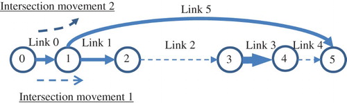
Figure 1 presents a small network to illustrate that the proposed model can give DUO results and that the route choices of different types of vehicles can differ. The network contains six nodes and six links. Node 0 is the origin and node 5 is the destination. Links 2 and 4 are bottleneck links (i.e. links with a limited design capacity) and marked with dashed lines. Other links are represented by thicker arrows and have a higher capacity. In this network, two links, that is, links 1 and 5, come out from node 1. At this node, there are two possible intersection movements: from link 0 to link 1 (intersection movement 1) and from link 0 to link 5 (intersection movement 2). If link 1 is used (i.e. intersection movement 1 is made), then links 2, 3, and 4 are also used before the destination is reached. If link 5 is used, then the vehicle reaches the destination directly, as link 5 is directly connected to the destination. The free-flow travel time on link 5 is longer than the sum of the free-flow travel times on links 1, 2, 3, and 4.

Figure 1. Small network.

Two vehicle classes, that is, cars and trucks, travel from origin node 0 to destination node 5. The demand for each class lasts for 50 intervals, where the first 30 intervals are peak intervals with higher demand. Table 1 lists all of the necessary network data.

Table 1. Input data for example 1.

(a) Link data
Link No.	Speed of cars (km/h)	Speed of trucks (km/h)	Length (km)	Density (veh/km)	Capacity (veh/h)	No. of lanes
0	72.0	36.0	0.02	200	3600	2
1	72.0	36.0	0.10	200	3600	2
2	72.0	36.0	1.30	200	1800	1
3	72.0	36.0	0.04	200	7200	4
4	72.0	36.0	0.06	200	3600	2
5	72.0	36.0	1.60	200	3600	2
(b) Demand data
	Car			Truck
OD pair	Input intervals	Demand (veh/h)		Input intervals	Demand (veh/h)
0–5	1–30	1200		1–30	900
	31–50	300		31–50	100

Table 2 demonstrates that the solution obtained satisfies the multi-class DUO conditions. To save space, we present only the proportions and travel times from intervals 5–15. The table shows that at any time interval and for any class of vehicle, if an approach proportion is positive, then the corresponding travel time to the destination equals the minimum travel time, implying that the multi-class DUO conditions are satisfied.

Table 2. Approach proportions and approach travel times under the DUO conditions.

t
5	1.00	76.0	0.00	81.0	76.0	1.00	156.0	0.00	162.0	156.0
6	1.00	76.7	0.00	81.0	76.7	1.00	156.6	0.00	162.0	156.6
7	1.00	77.3	0.00	81.0	77.3	1.00	157.1	0.00	162.0	157.1
8	1.00	78.0	0.00	81.0	78.0	1.00	157.0	0.00	162.0	157.0
9	1.00	78.7	0.00	81.0	78.7	1.00	157.0	0.00	162.0	157.0
10	1.00	79.3	0.00	81.0	79.3	1.00	157.0	0.00	162.0	157.0
11	1.00	80.0	0.00	81.0	80.0	1.00	157.0	0.00	162.0	157.0
12	1.00	80.7	0.00	81.0	80.7	1.00	157.0	0.00	162.0	157.0
13	0.56	81.0	0.44	81.0	81.0	1.00	157.0	0.00	162.0	157.0
14	0.00	81.0	1.00	81.0	81.0	1.00	157.0	0.00	162.0	157.0
15	0.00	81.0	1.00	81.0	81.0	1.00	157.0	0.00	162.0	157.0

The bold values emphasise that ‘if an approach proportion is positive, then the corresponding travel time to the destination equals the minimum travel time’.

The approach proportions of the two classes departing during the same time interval could be different. For example, and , indicating that the route choices for car and truck drivers are different. Such a distinction can be attributed to the difference in the travel speeds of different vehicle classes and selfish route choice behaviour, as different travel speeds result in different travel times associated with each link and selfish route choice behaviour generates different responses to these travel times. The discrepancy in the approach proportions and travel times indeed underlines the importance of considering multiple vehicle classes in a DTA model, as single-class models cannot capture diversity in route choices and travel times across different vehicle types. Without capturing the route choice of each vehicle type correctly, road restrictions or priority control for particular vehicle types cannot be implemented effectively.

Table 2 shows that the trucks do not change routes because intersection movement 1 is always chosen. However, the route choices and travel times of the car drivers vary over time. Figure 2 is plotted to investigate how the travel times and approach proportions of cars change over time. It is clear that the departure time intervals can be divided into five periods according to the minimum travel time.

Figure 2. Approach proportions associated with intersection movement 1 and minimum travel times of cars between nodes 1 and 5.

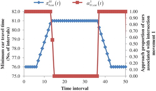
For the first six intervals, the approach proportions for intersection movement 1 equal 1.0 and the minimum car travel times associated with this movement are constant, implying that all of the cars departing during these intervals use intersection movement 1 and experience identical travel times. There are three reasons for this. First, after making intersection movement 1, the total free-flow travel time on links 1–4 is shorter than that on link 5. Second, given that the car demand itself is less than the capacity of either bottleneck link, the cars do not form a queue. Third, no trucks arrive at either bottleneck link concurrently with the cars departing before interval 6. Only the cars departing after interval 6¹ reach the tail of the first bottleneck link, that is, link 2, simultaneously with the trucks departing during interval 1. Hence, the total inflow (in PCU) is greater than the capacity of link 2. Consequently, not all of the vehicles can enter link 2, and a queue builds up on link 1.

The growth in queue length explains the increment in the minimum car travel times after interval 6, as observed in Figure 2. Nevertheless, despite the changes in the minimum car travel time, the approach proportion for intersection movement 1 is unvaried, as the travel time associated with intersection movement 1 is still less than that associated with intersection movement 2.

Until interval 13 (see Table 2), when the travel time associated with intersection movement 1 grows to a value equal to the travel time associated with intersection movement 2, some of the car drivers begin to use link 5 (downstream links for intersection movement 2). Between intervals 14 and 36, all of the car drivers give up link 1 and choose link 5, and the minimum car travel time becomes a constant and equals the travel time associated with intersection movement 2. There are two reasons for the constant minimum travel time. First, link 5 connects the destination node directly. Second, the travel time associated with intersection movement 1 is stabilised because there is a queue with a fixed length on link 1. This queue comprises only trucks and its fixed length results from the constant truck demand during peak intervals (i.e. the first 30 intervals). The car travel times and approach proportions do not change immediately after the peak intervals. A six-interval lag is observed because it takes six intervals for the trucks departing during the last interval of the peak period, that is, interval 30, to arrive at node 2. Therefore, during these lag intervals, the queuing delay on link 1 is still the same as that during the peak intervals.

It is only after the interval during which the trucks departing at interval 30 enter link 2 (i.e. after interval 36) that the minimum travel time and approach proportions of the cars begin to change. The demands for trucks and cars drop after interval 30, affecting the queue length on link 1. The car travel time drops due to the demand reduction. Car drivers use link 1 when the travel time from nodes 1 to 5 via link 1 is slower than the free-flow travel time on link 5.

The travel times and approach proportions eventually return to the initial state, that is, the state in which the network is free of queues, as the queue on link 1 dissipates.

4.2 Effects of truck demand and speed on the approach proportions and travel times of cars

4.2.1 Effects of truck demand on the approach proportions and travel times of cars

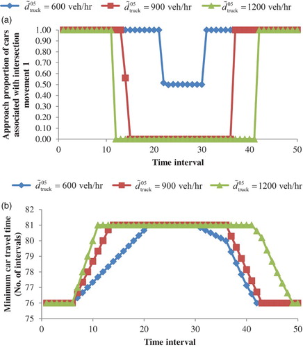
Based on the setting in subsection 4.1, we examine the effects of truck demand on the approach proportions and travel times of cars. Figure 3 plots the minimum car travel times and approach proportions associated with intersection movement 1 when the truck demand varies from 600 to 1200 veh/h. The effects can be grouped into three categories.

1. Truck demand affects the approach proportions of cars. As shown in Figure 3(a), when the truck demand increases to 900 or 1200 veh/h, all of the car drivers switch from links 1 to link 5 during the middle period, while some cars continue to travel via link 1 when the truck demand is maintained at 600 veh/h. Both the demands of trucks and cars using link 1 contribute to the total inflow into that link, decreasing the truck demand and allowing more cars to travel on link 1.

2. Truck demand affects the increasing rate of car travel time. Figure 3(b) shows that during the growth of the minimum car travel time from 76 to 81 intervals, the time increases faster at a higher demand level. The change in car travel time is rooted in the variation in the outflow rate for cars travelling on link 1, on which a queue is formed. The lower the car outflow rate, the longer the car travel time associated with link 1. According to Equation (41), the car outflow rate is directly proportional to the queue inflow rate and inflow capacity of downstream links and inversely proportional to the total outflow (in PCU). When the truck demand increases, the total outflow grows. As the car demand remains unchanged, the queue inflow rate does not increase compared with the case involving trucks. The inflow capacity of the downstream link remains the same. As a result, the car outflow rate decreases. Meanwhile, the larger the truck demand, the more the car outflow rate decreases. Therefore, a higher truck demand induces a larger decrease in the car outflow rate on link 1, raising the increasing rate of car travel time associated with link 1.

3. Truck demand influences the start and end time intervals and usage duration for the vehicles using link 5. Figure 3(a) shows that the approach proportion associated with intersection movement 1 changes from one to zero during the middle departure period, meaning that the approach proportion associated with intersection movement 2 changes from zero to one during the period. As explained in Section 4.1, the middle period during which the car drivers switch from link 1 to link 5 is the period during which the travel times associated with two intersection movements are equal. Following the second point, acknowledging that the travel time increases faster when the truck demand is higher, it takes fewer intervals for the travel time associated with intersection movement 1 to match that associated with intersection movement 2. Therefore, the car drivers who depart during earlier time intervals choose link 5 earlier. The end time interval and usage duration for the vehicles using link 5 increase with the truck demand because the travel time decreases at a slower rate when the truck demand is higher, and more time is required to dissipate the queue.

Figure 3. Effects of truck demand on the approach proportions and travel times of cars. (a) Effect of truck demand on the approach proportions of cars. (b) Effect of truck demand on the travel times of cars.

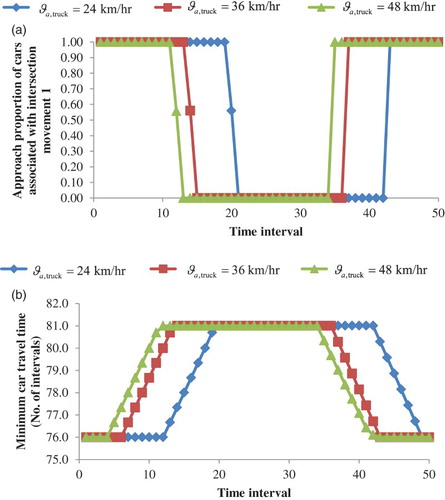
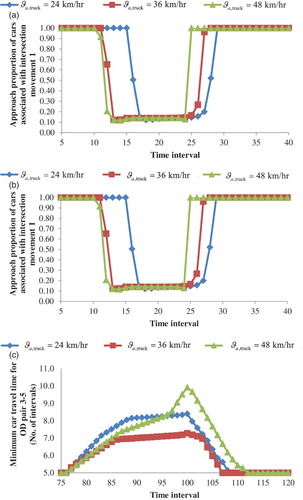
4.2.2 Effects of truck speed on the approach proportions and travel times of cars

The setting in this subsection is the same as that in the previous subsection, except that the truck demand is fixed at 900 veh/h while the truck speed varies from 24 to 48 km/h. The resultant approach proportions and travel times are plotted in Figure 4(a) and (b), respectively. Figure 4(b) shows that the time interval during which the travel time starts to increase is different. As the truck travel speed is higher, the trucks arrive at node 2 earlier. Accordingly, the start time intervals for a queue formed on link 1 occur earlier. The travel time begins to increase earlier, and the time interval during which the travel time associated with intersection movement 1 grows to that associated with intersection movement 2 occurs earlier. Therefore, the car drivers switch to link 5 during earlier time intervals, as shown in Figure 4(a).

Figure 4. Effects of truck speed on the approach proportions and travel times of cars. (a) Effect of truck speed on the approach proportions of cars. (b) Effect of truck speed on the travel times of cars.

4.3 Car–truck interaction paradox

4.3.1 Occurrence of the paradox

The following example reveals a car–truck interaction paradox in DTA. It shows that allowing trucks to travel in a network or increasing the demand of trucks travelling in a network can improve the network performance of cars in terms of their total travel time. We adopt the same network in Figure 1 and the same link data in Table 1(a). Two OD pairs are considered in this example, and the demand data are presented in Table 3.

Table 3. Demand data.

			Truck
	Car			Before	After
OD pair	Input intervals	Demand (veh/h)	Input intervals	Demand	Demand
0–5	5–30	1200	1–20	0 veh/h	1000 veh/h
0–5	31–40	300	–	–	–
3–5	75–100	3500	–	–	–
3–5	100–120	1500	–	–	–

We conduct a before-and-after study. In the before scenario, no trucks are allowed to travel in the network. In the after scenario, the demand of trucks for OD pair 0–5 is set at 1000 veh/h and lasts for 20 intervals. The total car travel times of the two scenarios are calculated and shown in Table 4. The result states that allowing trucks to enter the network decreases the total car travel time by 5.7%, from 980.0 to 924.1 intervals, indicating that the network performance of cars improves in terms of the total car travel time. The occurrence of the paradox is explained as follows.

Table 4. Occurrence of the multi-class paradox.

	Before	After	Improvement
Total car travel time (No. of intervals)	980.0	924.1	−5.7%

In the before scenario, cars travel via link 1 to the destination under the DUO conditions. When these cars arrive at node 4, a queue is formed on link 3, as the total inflow (in terms of the total PCU) into link 4, including the car demands of the two OD pairs, is larger than the capacity of link 4. Due to this queue, the travel time on link 3 increases. Given that link 3 is the only approach for the cars of OD pair 3–5 to reach the destination node, the car travel time for OD pair 3–5 rises. Meanwhile, the increase in car travel time for OD pair 3–5 depends on the number of cars entering link 3 from OD pair 0–5, as the demand of OD pair 3–5 is constant and less than the capacity of link 4. Hence, the more the cars of OD pair 0–5 use link 1, the greater the increase in car travel time for OD pair 3–5.

In the after scenario, all the trucks use link 1, as the resultant travel time to the destination is shorter for trucks. When the trucks arrive at node 2, a queue is induced on link 1. As a result, the car travel time associated with intersection movement 1 increases. When the travel time associated with intersection movement 1 equals that associated with intersection movement 2, some of the car drivers switch to link 5. The number of cars entering link 3 equivalently decreases compared with the number in the before scenario. The reduction mitigates the increase in car travel time for OD pair 3–5. In addition, the demand of OD pair 3–5 is far more than that of OD pair 0–5. Therefore, considering the whole network, although allowing trucks to travel between OD pair 0–5 increases the car travel time for OD pair 0–5, it decreases the total car travel time of the network by bringing down the car travel time for OD pair 3–5.

The trucks directly affect the car travel time for OD pair 0–5 and indirectly affect the car travel time for OD pair 3–5. The direct effect means that trucks interact with the cars of OD pair 0–5, and both the car and truck demands are responsible for the queue on link 1. In contrast, there is no interaction between the trucks of OD pair 0–5 and the cars of OD pair 3–5, as no trucks enter link 3 before interval 120, the last demand interval of OD pair 3–5, when the truck speed is 36 km/h. Therefore, the effect of trucks on the car travel time for OD pair 3–5 is considered indirect, that is, they affect the number of car drivers making intersection movement 1.

In reality, the before scenario may represent a traffic management scheme that restricts certain links or areas for trucks due to noise, weight, or height restrictions, assuming that such restrictions would benefit cars. However, the occurrence of the car–truck paradox implies that it is possible to relax the restriction so that the network performance for cars can be further improved in terms of the total car travel time.

4.3.2 Effects of truck demand and speed on the occurrence of the paradox

In this subsection, the effects of truck demand and speed on the occurrence of the paradox are elaborated based on the setting in the previous subsection. Table 5 presents an overview of the results. The value in a pair of brackets is the relative change in the total car travel time in relation to the total car travel time in the before scenario shown in Table 4. A negative number indicates that the total system car travel time decreases compared with that in the before scenario shown in Table 4. Table 5 offers three observations, which we summarise as follows.

Table 5. Effects of truck demand and speed on the total car travel time.

	Total car travel time (No. of intervals)
(veh/h)
200	980.0 (0.0%)	980.0 (0.0%)	980.0 (0.0%)
400	979.2 (−0.1%)	977.9 (−0.2%)	977.8 (−0.2%)
600	971.0 (−0.9%)	962.1 (−1.8%)	963.8 (−1.7%)
800	957.3 (−2.3%)	939.1 (−4.2%)	939.0 (−4.2%)
1000	948.5 (−3.1%)	924.1 (−5.7%)	919.8 (−6.1%)

First, Table 5 indicates that allowing trucks to enter the network may not change the total car travel time. This can also be considered a paradox. For instance, when the truck demand is 200 veh/h, the total car travel time is the same as that in the before scenario. A low truck demand is insufficient to incur a queue on link 1, and thus the car travel times for the two OD pairs are unaffected. In such a case, the network performance of trucks may be considered improved in terms of throughput.

Second, in addition to allowing trucks to travel in the network, increasing the demand of trucks may trigger the paradox. Consider the columns for the truck speed of 36 km/h. The total car travel time decreases when the truck demand increases from 200 to 1000 veh/h.

Third, truck demand and speed influence the magnitude of the changes in the total car travel time. In general, the difference in magnitude depends on the changes in the travel times of the two OD pairs. The changes vary under different truck speed and demand combinations. Figures 5 and 6 are plotted to clearly illustrate how the travel times of the two OD pairs vary. In Figure 5, the truck speed is fixed at 36 km/h. In Figure 6, the truck demand is set at 800 veh/h.

Figure 5. Effects of truck demand on the occurrence of the paradox. (a) Effect of truck demand on the approach proportions of cars in OD pair 0–5. (b) Effect of truck demand on the minimum car travel time for OD pair 0–5. (c) Effect of truck demand on the minimum car travel time for OD pair 3–5.

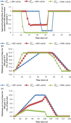
Figure 6. Effects of truck speed on the occurrence of the paradox. (a) Effect of truck speed on the approach proportions of cars in OD pair 0–5. (b) Effect of truck speed on the minimum travel time for OD pair 0–5. (c) Effect of truck speed on the minimum car travel time for OD pair 3–5.

4.3.3 Effects of truck demand and speed on the approach proportions and travel times of cars

Figures 5 and 6 plot the approach proportions and travel times of cars to visualise how car travel times and route choices change after trucks are introduced. The setting is basically the same as that in Subsection 4.3.1. In general, we conclude that truck demand and speed have similar effects as those observed in Figures 3 and 4. More specifically, Figures 5(a) and 6(a) show that the time interval at which the car drivers change their route is affected. Furthermore, Figures 5(b), 5(c), 6(b), and 6(c) demonstrate that the increasing and decreasing rates in the car travel times, represented by the slope of the travel time curve, are affected.

The following three observations are worth mentioning.

1. Figure 5(a) reveals a scenario in which increasing the truck demand may increase the proportion of cars travelling on the same link for certain intervals. More specifically, during intervals 23–26, the proportions of cars travelling on link 1 are larger when the truck demand is 200 veh/h, compared with the proportions when the truck demand is 600 veh/h.

2. Figure 5(b) indicates that a higher truck demand can decrease the minimum car travel time for the same OD pair. For example, between intervals 29 and 40, the car travel time for OD pair 0–5 drops with the increasing truck demand. Trucks induce different effects on the links with queues. Although increasing the truck demand directly increases the car travel time associated with link 1, it also indirectly decreases the car travel time associated with link 4. Considering the aggregate effect on the car travel time associated with intersection movement 1, the travel time decreases during intervals 29 and 40 along with the increasing truck demand.

3. In Figure 6(b), a kink at interval 12 is observed when the truck speed is 24 km/h. A queue is developed on link 1 after interval 12. The cars of OD pair 0–5 that depart before interval 12 encounter only one queue on link 3. There is no queue on link 1, as the cars that depart before interval 12 do not arrive at node 2 simultaneously with any truck when the truck speed is low. A queue is developed on link 1 only afterwards, when the trucks that depart during interval 1 arrive at node 2. Therefore, the car travel time increases further, as there is a longer queue after interval 12.

For OD pair 3–5, Figure 5(c) illustrates that the minimum car travel time drops when the truck demand rises. As explained in the occurrence of the paradox, the minimum travel time for OD pair 3–5 increases because many drivers of the cars in OD pair 0–5 decide to make intersection movement 1. Thus, when the truck demand increases, the number of cars using links 1–4 decreases, which in turn decreases the car travel time for OD pair 3–5.

Figure 6(c) shows that when the truck speed is 24 km/h, the travel time for OD pair 2 is higher than that when the truck speed is 36 km/h. When the truck speed is low, it takes more time intervals for trucks to arrive at node 2. Thus, all of the car drivers who depart earlier make intersection movement 1 and enter link 3, increasing the car travel time for OD pair 3–5 as a result. In addition, a sharp rise in the car travel time for OD pair 3–5 is observed when the truck speed is 48 km/h. The trucks enter link 3 when their speed is high, directly increasing the car travel time for OD pair 3–5.

4.3.4 Effects of background traffic levels on the occurrence of the paradox

To investigate the effect of various background traffic levels on the occurrence of the paradox, the network in Figure 1 is extended to that in Figure 7. Table 6 shows the link data. Three OD pairs are considered: OD pairs 0–5, 3–4, and 6–5. For OD pair 0–5, the demand data are identical to those in the paradox example. For OD pair 6–5, the car demand is set at 300 veh/h. The truck demand varies from 2400 to 3600 veh/h. Meanwhile, the route for the trucks travelling between nodes 6 and 5 is fixed, representing the scenario that trucks deliver goods following predefined tours with multiple stops. Table 7 reports the total car travel time (including the car travel times of OD pairs 0–5, 3–4, and 6–5) when the truck demand for OD pairs 0–5 and 6–5 varies. Similar to Table 5, a negative percentage in the brace means that the total car travel time decreases and the paradox occurs. The table shows that the paradox still occurs in most cases, despite the presence of background traffic.

Figure 7. Nine-node small network.

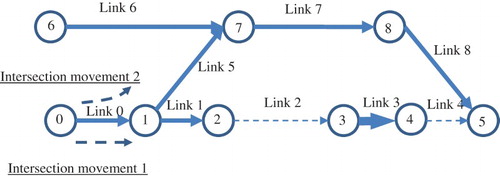
Table 6. Link data for Figure 7.

Link no.	Speed of cars (km/h)	Speed of trucks (km/h)	Length (km)	Density (veh/km)	Capacity (veh/h)	No. of lanes
0–4	Same as the data in Table 1
5	72.0	36.0	0.60	200	3600	2
6	72.0	36.0	0.06	200	7200	4
7	72.0	36.0	0.60	200	7200	4
8	72.0	36.0	0.40	200	7200	4

Table 7. Effect of background traffic levels on the occurrence of the paradox.

	(veh/h)
(veh/h)	2400	3600
200	1223.6 (−0.0%)	1237.2 (−0.0%)
400	1221.5 (−0.2%)	1234.5 (−0.2%)
600	1207.2 (−1.3%)	1222.4 (−1.2%)
800	1189.2 (−2.8%)	1212.6 (−2.0%)
1000	1181.7 (−3.4%)	1208.6 (−2.3%)

4.4 Performance of the solution algorithm

4.4.1 Effect of background traffic levels on the performance of the solution algorithm

To test the performance of the solution algorithm under various background traffic levels, we adopt the Nguyen–Dupuis network shown in Figure 8. The link length and density are the same as those seen in a study by Long et al. (2013). Four OD pairs are considered: 1–2, 1–3, 4–2, and 4–3. The car demand for each OD pair is set at 900 veh/h, and the truck demand is 600 veh/h. Meanwhile, three OD pairs, that is, 12–7, 5–8, and 9–11, are set as the OD pairs generating traffic in the network. The car demand for these OD pairs is fixed at 300 veh/h. The truck demand level varies from 150 to 750 veh/h. In the test, the stepsizes for the algorithm are set at and . The algorithm terminates if it does not converge to after evaluating 500 generated intermediate solutions. The number of intermediate solutions evaluated is adopted as the measurement for computational effort, as most of the calculation time is spent on evaluating a solution, which requires DNL.

Table 8 presents the effect of background traffic levels on the performance of the algorithm. In general, the increment in truck demand induces an additional computational effort for the algorithm to converge. Nevertheless, when the truck demand increases from 150 to 750 veh/h, only 24 additional intermediate solutions must be generated and evaluated. Such a computational burden is not significant and believed to be acceptable.

Table 8. Effect of background traffic levels on the performance of the solution algorithm.

	Truck demand for OD pairs 12–8, 5–8, and 9–11
	150 (veh/h)	300 (veh/h)	450 (veh/h)	600 (veh/h)	750 (veh/h)
Number of intermediate solutions evaluated	32	37	43	47	56

4.4.2 Convergence on the Sioux Falls network

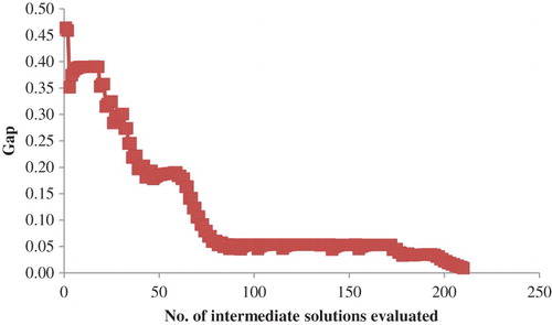
We demonstrate the performance of the solution algorithm using the Sioux Falls network, shown in Figure 9. The link and demand data are modified from the transportation network dataset maintained by Bar-Gera (2015). The link lengths are the same as those of the original dataset. For each OD pair and each departure time interval, the car demand (in vph) is one-sixth and the truck demand is one-twelfth of the original hourly demand (in vph). The demand lasts for 30 intervals, and each time interval is 30 s long. Density and speed are not provided in the original data. The density of each link is set at 200 veh/km, and the car and truck speeds are set at 72 and 54 km/h, respectively. Figure 10 plots the convergence curve. After evaluating 210 intermediate solutions, the algorithm converges below 0.01. The curve fluctuates because the mapping function may not be pseudomonotone.

Figure 8. The Nguyen and Dupuis network.

Figure 9. The Sioux Falls network.

Figure 10. Convergence of the algorithm on the Sioux Falls network.

5. Conclusions

This paper proposes an intersection-movement-based formulation for the multi-class DTA problem, wherein the adopted DNL model captures dynamic queuing and spillback effects. The problem is formulated as a VI problem and solved using an extragradient method. Path enumeration and path-set generation can be avoided in the solution procedure. Numerical studies are conducted to illustrate that the resulting solution of the VI satisfies the multi-class DUO conditions. Meanwhile, we demonstrate that changes in truck demand and speed affect the route choices and travel times of cars. These results underline the importance of capturing multiple vehicle types and their interactions in a DTA model. In addition, we demonstrate the performance of the proposed algorithm using the Nguyen and Dupuis network and the Sioux Falls network.

This paper also illustrates a car–truck interaction paradox in the context of DTA or, more generally, the interaction paradox between vehicles of different sizes. It states that allowing larger vehicles to travel or increasing the demand of such vehicles in a network can decrease the total travel time of smaller vehicles. The occurrence of the paradox is elaborated and the effects of truck demand and speed on that occurrence are investigated. Moreover, taking into account the increase in the throughput for trucks in the network, the overall performance of each class of vehicles improves, although the performance measure for cars is total travel time, which is different from that for trucks. These findings have important implications for traffic management and open up various new research directions, such as developing an optimal real-time, multi-class traffic management scheme, detecting the occurrence of a car–truck interaction paradox in a network, or simultaneously optimising the overall performance for each vehicle class.

We develop our model based on the classical DUO principle, where the main factor that affects route choice is travel time. In reality, a driver may consider other factors such as distance and number of signalised junctions when making route choice decisions. The route choice principle in this model can be replaced with more sophisticated and realistic principles without encountering fundamental difficulties. We leave this generalisation to future studies.

Acknowledgements

The authors are grateful to the four reviewers for their constructive comments.

Disclosure statement

No potential conflict of interest was reported by the authors.

ORCiD

Yu Jiang http://orcid.org/0000-0001-9461-633X

W. Y. Szeto http://orcid.org/0000-0001-7059-3532

Ke Han http://orcid.org/0000-0003-3529-6246

Additional information

Funding

This work is jointly supported by the National Natural Science Foundation of China [grant number 71271183]; a grant from the Research Grants Council of the Hong Kong Special Administrative Region, China [grant number HKU 716312E]; and University Research Committee of the University of Hong Kong [grant numbers 201211159009 and 201311159123].

Notes

1. The length between nodes 0 and 2 is 0.12 km. It takes 12 intervals for cars and 6 intervals for trucks to travel this length. Thus, the trucks that depart during interval 1 arrive simultaneously with the cars that depart during interval 6.

Appendix

This appendix shows that the approach-based DUO conditions (23) and (24) imply the link-based DUO conditions (1) and (2). The proof contains two parts:

Part 1: Condition (23) implies condition (1).

For OD pair id, the demand rate is input and known. Thus, we can consider the following two cases.

Case 1: . By multiplying to both sides of the if-conditions in Equation (23), we can obtain (A1) which can be simplified to condition (1) according to condition (21).

Case 2: . In this case, after multiplying to both sides of the if-conditions in Equation (23), the two if-conditions reduce to , which can be further simplified to a special case of (A1), that is, , according to Equation (21).

Combining the above two cases, it is concluded that if condition (23) holds, then no matter the value of , condition (1) holds.

Part 2: Condition (24) implies condition (2).

Although is a decision variable and cannot be determined in advance, it can be known by network loading once an approach-based DUO solution is obtained. Therefore, given an approach-based DUO solution that satisfies (23) and (24), we can consider two cases.

Case 1: . We can multiply to both sides of the if-conditions in Equation (24) and obtain (A2) which can be simplified to condition (2) according to Equation (22).

Case 2: . In this case, after multiplying to both sides of the if-conditions in Equation (24), the two if-conditions reduce to , which can be further simplified to , a special case of (A2), according to Equation (22).

Combining the above two cases, it is concluded that if condition (24) holds, then condition (2) holds.

From the above two parts, it is concluded that the approach-based DUO conditions (23)–(24) imply the link-based DUO conditions (1)–(2). This completes the proof.

References

- Ban, X. J., H. X. Liu, M. C. Ferris, and B. Ran. 2008. “A Link-Node Complementarity Model and Solution Algorithm for Dynamic User Equilibria with Exact Flow Propagations.” Transportation Research Part B: Methodological 42 (9): 823–842. doi: 10.1016/j.trb.2008.01.006
- Ban, X. J., J. S. Pang, H. X. Liu, and R. Ma. 2012a. “Continuous-Time Point-Queue Models in Dynamic Network Loading.” Transportation Research Part B: Methodological 46 (3): 360–380. doi: 10.1016/j.trb.2011.11.004
- Ban, X. J., J. S. Pang, H. X. Liu, and R. Ma. 2012b. “Modeling and Solving Continuous-Time Instantaneous Dynamic User Equilibria: A Differential Complementarity Systems Approach.” Transportation Research Part B: Methodological 46 (3): 389–408. doi: 10.1016/j.trb.2011.11.002
- Bar-Gera, H. 2015. “Transportation Network Test Problems.” Accessed June 29, 2015. http://www.bgu.ac.il/~bargera/tntp/.
- Bliemer, M. C. J. 2005. INDY 2.0 Model Specifications. Delft University of Technology. working paper, The Netherlands.
- Bliemer, M. C. J. 2007. “Dynamic Queuing and Spillback in Analytical Multi-Class Dynamic Network Loading Model.” Transportation Research Record: Journal of the Transportation Research Board 2029 (1): 14–21. doi: 10.3141/2029-02
- Carey, M. 1987. “Optimal Time-Varying Flows on Congested Networks.” Operations Research 35 (1): 58–69. doi: 10.1287/opre.35.1.58
- Carey, M., and D. Watling. 2012. “Dynamic Traffic Assignment Approximating the Kinematic Wave Model: System Optimum, Marginal Costs, Externalities and Tolls.” Transportation Research Part B: Methodological 46 (5): 634–648. doi: 10.1016/j.trb.2012.01.008
- Chen, H. K., and C. F. Hsueh. 1998. “A Model and an Algorithm for the Dynamic User-Optimal Route Choice Problem.” Transportation Research Part B: Methodological 32 (3): 219–234. doi: 10.1016/S0191-2615(97)00026-X
- Chow, A. H. F. 2009a. “Dynamic System Optimal Traffic Assignment – A State-Dependent Control Theoretic Approach.” Transportmetrica 5 (2): 85–106. doi: 10.1080/18128600902717483
- Chow, A. H. F. 2009b. “Properties of System Optimal Traffic Assignment with Departure Time Choice and Its Solution Method.” Transportation Research Part B: Methodological 43(3): 325–344. doi: 10.1016/j.trb.2008.07.006
- Friesz, T. L., D. Bernstein, T. E. Smith, R. L. Tobin, and B. W. Wie. 1993. “A Variational Inequality Formulation of the Dynamic Network User Equilibrium Problem.” Operations Research 41 (1): 179–191. doi: 10.1287/opre.41.1.179
- Friesz, T. L., K. Han, P. A. Neto, A. Meimand, and T. Yao. 2013. “Dynamic User Equilibrium Based on a Hydrodynamic Model.” Transportation Research Part B: Methodological 47 (1): 102–126. doi: 10.1016/j.trb.2012.10.001
- Friesz, T. L., J. Luque, R. L. Tobin, and B. W. Wie. 1989. “Dynamic Network Traffic Assignment Considered as a Continuous Time Optimal Control Problem.” Operations Research 37 (6): 893–901. doi: 10.1287/opre.37.6.893
- Friesz, T. L., and A. Meimand. 2014. “A Differential Variational Inequality Formulation of Dynamic Network User Equilibrium with Elastic Demand.” Transportmetrica A: Transport Science 10 (7): 661–668. doi: 10.1080/18128602.2012.751684
- Han, K., T. L. Friesz, and T. Yao. 2013a. “A Partial Differential Equation Formulation of Vickrey’s Bottleneck Model, Part I: Methodology and Theoretical Analysis.” Transportation Research Part B: Methodological 49: 55–74. doi: 10.1016/j.trb.2012.10.003
- Han, K., T. L. Friesz, and T. Yao. 2013b. “A Partial Differential Equation Formulation of Vickrey’s Bottleneck Model, Part II: Numerical Analysis and Computation.” Transportation Research Part B: Methodological 49: 75–93. doi: 10.1016/j.trb.2012.10.004
- Han, K., T. L. Friesz, and T. Yao. 2013c. “Existence of Simultaneous Route and Departure Choice Dynamic User Equilibrium.” Transportation Research Part B: Methodological 53: 17–30. doi: 10.1016/j.trb.2013.01.009
- Huang, H. J., and W. H. K. Lam. 2002. “Modeling and Solving the Dynamic User Equilibrium Route and Departure Time Choice Problem in Network With Queues.” Transportation Research Part B: Methodological 36 (3): 253–273. doi: 10.1016/S0191-2615(00)00049-7
- Lo, H. K., and W. Y. Szeto. 2002a. “A Cell-Based Variational Inequality Formulation of the Dynamic User Optimal Assignment Problem.” Transportation Research Part B: Methodological 36 (5): 421–443. doi: 10.1016/S0191-2615(01)00011-X
- Lo, H. K., and W. Y. Szeto. 2002b. “A Cell-Based Dynamic Traffic Assignment Model: Formulation and Properties.” Mathematical and Computer Modelling 35 (7–8): 849–865. doi: 10.1016/S0895-7177(02)00055-9
- Lo, H. K., and W. Y. Szeto. 2004. “Modeling Advanced Traveler Information Services: Static Versus Dynamic Paradigms.” Transportation Research Part B: Methodological 38 (6): 495–515. doi: 10.1016/j.trb.2003.06.001
- Lo, H. K., and W. Y. Szeto. 2005. “Road Pricing for Hyper-congestion.” Transportation Research Part A 39 (7–9): 705–722.
- Long, J. C., Z. Y. Gao, and W. Y. Szeto. 2011. “Discretised Link Travel Time Models Based on Cumulative Flows: Formulations and Properties.” Transportation Research Part B: Methodological 45 (1): 232–254. doi: 10.1016/j.trb.2010.05.002
- Long, J. C., H. J. Huang, Z. Y. Gao, and W. Y. Szeto. 2013. “An Intersection-Movement-Based Dynamic User Optimal Route Choice Problem.” Operations Research 61 (5): 1134–1147. doi: 10.1287/opre.2013.1202
- Long, J. C., W. Y. Szeto, H. J. Huang, and Z. Y. Gao. 2015a. “An Intersection-Movement-Based Stochastic Dynamic User Optimal Route Choice Model for Assessing Network Performance.” Transportation Research Part B: Methodological 74: 182–217. doi: 10.1016/j.trb.2014.12.008
- Long, J. C., W. Y. Szeto, Q. Shi, Z. Y. Gao, and H. J. Huang. 2015b. “A Nonlinear Equation System Approach to the Dynamic Stochastic User Equilibrium Simultaneous Route and Departure Time Choice Problem.” Transportmetrica A: Transport Science 11 (5): 388–419. doi: 10.1080/23249935.2014.1003112
- Ma, R., X. J. Ban, and J.-S. Pang. 2014a. “Continuous-time Dynamic System Optimum for Single-Destination Traffic Networks with Queue Spillbacks.” Transportation Research Part B: Methodological 68: 98–122. doi: 10.1016/j.trb.2014.06.003
- Ma, R., X. J. Ban, and J.-S. Pang. 2014b. “Continuous-time Dynamic User Equilibrium Model with Departure-Time Choice and Capacitated Queue.” Proceedings of the 5th International Symposium on Dynamic Traffic Assignment, Salerno, Italy, 17–19 June.
- Mahmassani, H. S., T. Hu, and R. Jayakrishnan. 1992. “Dynamic Traffic Assignment and Simulation for Advanced Network Informatics (DYNASMART).” Proceedings of the 2nd international CAPRI seminar on Urban Traffic Networks. Capri, July.
- Mahut, M., and M. Florian. 2010. “Traffic Simulation with Dynameq.” In Fundamentals of Traffic Simulation, edited by Jaume Barceló, 323–361. New York: Springer.
- Meng, Q., and H. L. Khoo. 2012. “A Computational Model for the Probit-Based Dynamic Stochastic User Optimal Traffic Assignment Problem.” Journal of Advanced Transportation 46 (1): 80–94. doi: 10.1002/atr.149
- Merchant, D. K., and G. L. Nemhauser. 1978a. “A Model and an Algorithm for the Dynamic Traffic Assignment Problems.” Transportation Science 12 (3): 183–199. doi: 10.1287/trsc.12.3.183
- Merchant, D. K., and G. L. Nemhauser. 1978b. “Optimality Conditions for a Dynamic Traffic Assignment Model.” Transportation Science 12 (3): 200–207. doi: 10.1287/trsc.12.3.200
- Mun, J. S. 2007. “Traffic Performance Models for Dynamic Traffic Assignment: An Assessment of Existing Models.” Transport Reviews 27 (2): 231–249. doi: 10.1080/01441640600979403
- Ngoduy, D. 2010. “Multi-Class First-Order Modelling of Traffic Networks Using Discontinuous Flow-Density Relationships.” Transportmetrica 6 (2): 121–141. doi: 10.1080/18128600902857925
- Peeta, S., and A. K. Ziliaskopoulos. 2001. “Foundations of Dynamic Traffic Assignment: The Past, the Present and the Future.” Networks and Spatial Economics 1 (3–4): 233–265. doi: 10.1023/A:1012827724856
- Perakis, G., and Roels, G. 2006. “An Analytical Model for Traffic Delays and the Dynamic User Equilibrium Problem.” Operations Research 54 (6): 1151–1171. doi: 10.1287/opre.1060.0307
- Ran, B., and D. E. Boyce. 1996. Modeling Dynamic Transportation Network: An Intelligent Transportation System Oriented Approach. Springer: Heidelberg.
- Ran, B., D. E. Boyce, and L. J. LeBlanc. 1993. “A New Class of Instantaneous Dynamic User-Optimal Traffic Assignment Models.” Operations Research 41 (1): 192–202. doi: 10.1287/opre.41.1.192
- Szeto, W. Y.. 2008. “Enhanced Lagged Cell-Transmission Model for Dynamic Traffic Assignment.” Transportation Research Record: Journal of the Transportation Research Board 2085: 76–85. doi: 10.3141/2085-09
- Szeto, W. Y., and Y. Jiang. 2014. “Transit Assignment: Approach-Based Formulation, Extragradient Method, and Paradox.” Transportation Research Part B: Methodological 62: 51–76. doi: 10.1016/j.trb.2014.01.010
- Szeto, W. Y., Y. Jiang, and A. Sumalee. 2011. “A Cell-Based Model for Multi-Class Doubly Stochastic Dynamic Traffic Assignment.” Computer-Aided Civil and Infrastructure Engineering 26: 595–611. doi: 10.1111/j.1467-8667.2011.00717.x
- Szeto, W. Y., and H. K. Lo. 2004. “A Cell-Based Simultaneous Route and Departure Time Choice Model with Elastic Demand.” Transportation Research Part B: Methodological 38 (7): 593–612. doi: 10.1016/j.trb.2003.05.001
- Szeto, W. Y., and H. K. Lo. 2005. “Dynamic Traffic Assignment: Review and Future Research Directions.” Journal of Transportation Systems Engineering and Information Technology 5 (5): 85–100.
- Szeto, W. Y., and H. K. Lo. 2006. “Dynamic Traffic Assignment: Properties and Extensions.” Transportmetrica 2 (1): 31–52. doi: 10.1080/18128600608685654
- Szeto, W. Y., and S. C. Wong. 2012. “Dynamic Traffic Assignment: Model Classifications and Recent Advances in Travel Choice Principles.” Central European Journal of Engineering 2 (1): 1–18.
- Wie, B. W., R. L. Tobin, and M. Carey. 2002. “The Existence, Uniqueness and Computation of an Arc-Based Dynamic Network User Equilibrium Formulation.” Transportation Research Part B: Methodological 36 (10): 897–918. doi: 10.1016/S0191-2615(01)00041-8
- Yagar, S. 1971. “Dynamic Traffic Assignment by Individual Path Minimisation and Queuing.” Transportation Research 5 (3): 179–196. doi: 10.1016/0041-1647(71)90020-7