Pedestrian dynamics at transit stations: an integrated pedestrian flow modeling approach

ABSTRACT

This paper presents an integrated modelling framework to capture pedestrian walking behaviour in congested and uncongested conditions. The framework is built using a combination of concepts from the Social Force model (basic one-to-one interaction), behavioural heuristics (physiological and cognitive constraints), and materials science (multi-body potential concept). The approach is ultimately designed to capture pedestrian interactions in transit stations. Due to the lack of available trajectory data of pedestrians within transit stations, the model is calibrated using pedestrian trajectory data from narrow bottleneck and bidirectional flow experiments provided by the Delft University of Technology. These two scenarios were chosen due to the frequency with which they occur in transit stations. The integrated modelling framework reproduced similar trajectory patterns observed in the experiments which encouraged a transit station simulation in an environment similar to that at the Foggy-Bottom METRO station in Washington, D.C.

KEYWORDS:

• Integrated microscopic model
• pedestrian walking behavior
• trajectory data
• transit stations

1. Introduction and motivation

Pedestrians play an increasingly important role in the traffic scenes of the modern world. This role is particularly important in urban areas, such as Washington D.C., where pedestrians often dominate the traffic flow (District of Columbia Department of Transportation). By accurately modeling pedestrian behavior, design of civil infrastructures may be improved while increasing the number of pedestrians who can safely flow through the corresponding geometric components (i.e. pedestrian infrastructure capacity). Of particular interest is the flow of pedestrians through public transit stations (Daamen 2004; Zhang et al. 2009; Hänseler et al. 2013). Transit stations must be able to hold large numbers of travelers while also allowing pedestrians to move safely and efficiently from one location to another. Accurately modeling pedestrian behavior through transit stations allows identifying areas with critical densities that might be dealt with through changing the corresponding geometric features or through offering some level of control (pre-timed or real-time). Many models of pedestrian behavior have been previously suggested, however a relatively recent review of crowd models conducted in 2013 by Duives et al. suggested that model usability is highly dependent on the application for which the model was originally developed (Duives, Daamen, and Hoogendoorn 2013). In this paper, the model is intended to be used for crowd management and control for the Washington, DC METRO system. As such, the model must be able to accurately show high density situations, run in real-time, and consider the complex nature of human decision-making. Some existing computationally efficient models have been developed; however, these models frequently capture one-to-one interactions and fail to consider the complexities of decision-making that occur in crowded conditions (Tao and Jun 2009; Jian et al. 2014). Other models such the Optimal Reciprocal Collision Avoidance Model (Van Den Berg et al. 2011), the hybrid Zanlungo, Ikeda, and Kanda (2011) Social Force (SF) model, and Crociani and Lämmel’s model (2016) are both computationally efficient and consider complex decision-making dimensions such as learning. This paper does not intend to criticize such models but to offer an alternative that might have flexibility for the addition of modules that capture crowd interactions at transit stations.

Accordingly, the objective of this paper is to accurately and efficiently model pedestrian operational behavior (focusing on walking behavior), using a combination of the Social Force model (Helbing and Molnár 1995), the behavioral heuristics model (Moussaïd, Helbing, and Theraulaz 2011), and concepts from materials science such us multi-body potential molecular interactions (Gniewek et al. 2011). The motivation behind such ‘integration’ is the hope that the resulting ‘integrated model’ (IM) will benefit from the attraction/repulsive force concepts offered by the social force models (offering realistic one-to-one interactions), the flexibility of the behavioral heuristics (incorporating multiple psychological and physiological pedestrian characteristics), and the theoretical foundation from materials science. Furthermore, the combination of these principles allows for drawbacks of either model to be corrected with aspects from the other model. Toward realizing this objective, the basic interaction between ‘bodies’ (i.e. pedestrians or obstacles) is adapted from the Social Force model (Helbing and Molnár 1995). The Social Force model essentially uses Newtonian physics to describe how pedestrians move. The model defines attractive and repellant forces which push and pull pedestrians along their path of motion. On the other hand, the behavioral heuristics model utilized in this paper considers that pedestrians take advantage of their eyesight and cognitive perception of their surrounding environment to determine which direction is the most efficient to reach their local destination (i.e. operational navigation) (Moussaïd, Helbing, and Theraulaz 2011). Finally, an essential concept from materials science is incorporated; this concept states that molecular interactions can be well modeled by taking into account directly neighboring molecules. This greatly simplifies the complexity of the calculations since not all surrounding objects need to be considered. This conceptual hypothesis is to be tried in this paper: when applied to pedestrian dynamics, this concept implies that accurately modeling pedestrian behavior requires ‘social force’ calculations not only between the two closest bodies (i.e. pedestrians or obstacles), nor all surrounding bodies, but rather between multiple bodies (i.e. multi-body potential interactions) within the corresponding field of view (Gniewek et al. 2011). In our model, we experimented with considering the closest 1, 2, and 3 nearest pedestrians/obstacles when determining a specific pedestrian’s course of action. It should be noted that this number may be a parameter to be calibrated depending on surrounding traffic conditions.

The IM rules are programmed in a Java simulation platform constructed by the authors. Realistic parametric values were initially taken from the literature and later calibration efforts were conducted using experimental data obtained by the Transport and Planning Department at the Delft University of Technology (TU Delft). The basic manual calibration was aimed to minimize trajectory error between the modeled results and the experimental results using the bi-directional and narrow bottleneck experiments. Afterwards, a simulation study was conducted to look into crowd phenomena that might be seen at the Foggy-Bottom METRO station in Washington, D.C. (USA). A brief literature on microscopic pedestrian modeling is presented in the next section, followed by an explanation of the IM approach suggested in this paper. Section 3 presents the model itself, including a description of the model’s formulation and basic calibration. Section 4 contains an analysis of the results obtained from model trajectory calibration and the simulation of pedestrian movement in a transit station. In Section 5, the paper concludes and suggests future research recommendations.

2. Background

Microscopic pedestrian traffic models describe the movement of individual pedestrians and attempt to simulate crowd dynamics by considering the choices made by individuals. These models may aim to capture the strategic behavior of pedestrians (choice of activities and the corresponding departure time and destination), the tactical behavior of pedestrians (route choice and possible related activity scheduling), and the operational behavior of pedestrians (walking, waiting, and local navigation). Focusing on the operational pedestrian behavior, among the microscopic modeling approaches which are the most prominent and closely related to the model discussed in this paper, there are Cellular Automata (CA), Social Force (SF), and behavioral heuristics (BH) models.

In the CA modeling approach, the available walking space is divided into a grid (i.e. cells) and pedestrians are able to move among grid spaces based on rules that vary between models proposed by different authors (Blue, Embrechts, and Adler 1997). Generally, each cell can hold a pedestrian or be empty, and full cells cannot be entered by other pedestrians. These models are computationally efficient because time and space are both discrete. However, the rules that define walking behavior are not based on human decision-making and behavioral capabilities. The CA rules can become complex increasing the corresponding estimation tractability as well as the difficulty involved with calibration (Helbing et al. 2005). Moreover, CA models have been criticized due to their inability to show phenomena observed at high densities, like clogging and turbulence (Helbing et al. 2005). Nevertheless, it remains a popular model with improved model suggestions being published on a yearly basis. For example, the recent work of Flötteröd and Lämmel (2015) and Crociani and Lämmel (2016) offered a CA model with rules derived from behavioral observations and that can re-create multiple real-life congestion dynamics.

The SF modeling theory, first suggested by Helbing and Molnár, is a physics-based approach that describes pedestrian motion through three relatively simple parameters (Helbing and Molnár 1995). These parameters are incorporated into equations that capture a pedestrian’s ‘internal motivation to perform certain movements’. The first parameter represents a pedestrian’s acceleration toward her/his desired velocity. The second parameter relates to a pedestrian’s desire to remain at a certain distance away from borders, obstacles, and other pedestrians (i.e. comfort space). The third parameter quantifies the attractiveness that a pedestrian may feel when approaching familiar pedestrians, store windows, etc. Some expansions and variations of the equations first proposed by Helbing and Molnar have been suggested (Johansson 2004). Perhaps the greatest difficulty with this model is correctly calibrating the SF equations in order to accurately recreate organizational phenomena that have been observed in the real world. Furthermore, the ability of a physics-based approach to accurately predict human behavior (which is stochastic by nature) has been questioned. Because of these difficulties, physics-based modeling approaches have been questioned. Their increasing computational complexity and the extensive calibration efforts needed have prompted researchers to develop more simplistic modeling approaches. Accordingly, some researchers advocate for simpler modeling theories to efficiently capture pedestrian behavior and crowd dynamics.

One such group of models which attempts to simplify the microsimulation of pedestrian movements while still covering the fundamental observed behaviors is the behavioral heuristic models. The first proposed model that incorporates elements of BH was developed by Paris, Pettré, and Donikian (2007). Although their approach does not describe itself as a BH model, it includes pedestrians’ ability to predict future collisions, which Moussaïd et al. later classify as a heuristic (Moussaïd, Helbing, and Theraulaz 2011). Moussaïd et al. propose a modeling approach based on what they term ‘behavioral heuristics’ (Moussaïd, Helbing, and Theraulaz 2011). BH are cognitive procedures used when decisions have to be made quickly. The suggested heuristics are based on the following two questions: (1) what kind of information is used by pedestrians? (2) How does this information influence walking behavior? To answer these questions, it is assumed that vision is the main source of information for pedestrians. As such, the first heuristic becomes ‘A pedestrian chooses the direction that allows the most direct path to their destination, taking into account the presence of obstacles’ (Moussaïd, Helbing, and Theraulaz 2011). The second heuristic is ‘A pedestrian maintains a distance from the first obstacle in the chosen walking direction that ensures a time to collision of at least τ’ (Moussaïd, Helbing, and Theraulaz 2011). The BH models are capable of showing crowd turbulence in high density situations.

As has been mentioned, one of the primary difficulties associated with modeling pedestrian behavior stems from the complexity of calibration. Model calibration has been achieved through a variety of methods. The most basic method, of course, is simple manual calibration, in which parameters are manually altered in order to adjust model output until satisfactory results are obtained. More advanced methods for model calibration range from applying statistical estimation methods, such as Maximum Likelihood Estimation (MLE) (Hoogendoorn and Daamen 2007; Ko, Kim, and Sohn 2013) to evolutionary adjustment to video tracking data (Johansson et al. 2008), among others. Both MLE and evolutionary adjustment to video data have had success in calibrating the SF model. MLE is a statistical method that is used to estimate the parameters of the model. This method, as described by Ko, Kim, and Sohn (2013), uses observed individual trajectory data to estimate the model parameters, although MLE can also be applied to macroscopic pedestrian characteristics. The underlying principle of MLE is that the observed data are those which correspond to the most probable scenario. MLE allows for the simultaneous estimation of all parameter coefficients and produces unbiased estimates (Lehmann and Casella 1998). The evolutionary adjustment to video tracking data conducted by Johansson, Helbing, and Shukla (2007) made use of an evolutionary optimization algorithm that determined the best parameter specifications for the SF model. The authors use a hybrid method to combine empirical trajectory data and microscopic simulation data of pedestrian movement in space by assigning a virtual pedestrian in the model to every real pedestrian observed in the video data. The authors used distance error to determine how well the model was performing, with the best possible fitness value corresponding to 0. The authors then used an evolutionary algorithm to obtain the parameter set with the best fitness value. The authors found that there was actually a broad range of parameter sets that produced similarly good results. In this exploratory paper, the presented model has undergone a basic manual calibration using pedestrian flow data collected in five scenarios, as further described in Section 5.

In summary, the models discussed in this section are each capable of reproducing particular aspects of crowd dynamics. However, the complexities involved in real world crowds have prevented the creation of a single model which is capable of reproducing all crowd phenomena. Although this is a limitation, models can still be developed for specific causes. For the model presented here, the ultimate objective is to achieve realistic results in high density situations, since these are the scenarios in which METRO personnel would need to deploy the crowd control devices at their disposal. Of course, this ultimate objective also relies on maintaining the efficiency of real-time computation. However, the limited availability of high density data increases the difficulty of attaining this objective. Therefore, the preliminary goal of this paper is to show that the integrated modeling approach, which combines aspects of SF, BH, and materials science is capable of reproducing different flow dynamics obtained through experimentation at TU Delft. As such, the main contribution becomes the combination of a continuous space SF simulation model and a heuristic approach (inspired by/derived from physiological perception considerations and materials science) to capture realistic behaviors in different set-ups/experiments. Such hybrid approach could be utilized with other force-based models (e.g. generalized centrifugal-force model) or velocity–space based models (e.g. ORCA).

The methodology utilized in this paper is explained in the next section focusing on the model formulation and basic calibration. For validation reasons, the simulation numerical results are presented afterwards before concluding with future research recommendations.

3. Model formulation and calibration

In this section, the IM-related details are explained, beginning with the formulation which specifies the aspects of the suggested model which were adapted from other sources as well as the method by which they were combined. Following the formulation, the calibration efforts that were undertaken for this model are described.

3.1. Formulation

The primary equations used in this model come from the SF and BH models and are combined using concepts from materials science. The acceleration term affecting pedestrians whose actual velocity differs from their desired velocity comes from the SF model, as shown: (1) where , , , and .

The relaxation time accounts for the time taken by a pedestrian to return to his/her desired speed. The direction chosen by a pedestrian is dictated by the BH model’s first heuristic, which essentially states that a pedestrian chooses the direction that allows for the most direct path to his/her destination while considering the presence of other pedestrians and obstacles (Moussaïd, Helbing, and Theraulaz 2011). To compute this direction, the distance to the first collision, is computed for all pedestrians within a pedestrian’s field of view. If no collision is expected to occur, then is set to a default maximum value d_max. The d_max value corresponds to the ‘horizon distance’ of the pedestrian, namely how far ahead the pedestrian is looking while deciding which direction to move in. It should be noted that this ‘heuristic’ component may add to the repulsive/attractive forces experienced through the interaction between pedestrians. The directional equation is shown in Equation (2). (2) where , , , , and

The repulsive effect felt by the pedestrian as a result of nearby obstacles and pedestrians is described by the SF model. Equation (3) shows the repulsive effect caused by other pedestrians, β. (3) where , , and .

The monotonic decreasing function of b(·) has equipotential lines in the form of an ellipse that is pointed in the direction of motion, which accounts for a pedestrian’s next step in the specified direction. This feature is included because other pedestrians take into account the imminent step of the other pedestrian, assuming the other pedestrians maintain their current speed (Van Den Berg et al. 2011). The semi-minor axis of the ellipse is denoted by b, as shown in Equation (4). (4) where , , and _.

The repulsive potential is assumed to decrease exponentially, as shown in Equation (5). (5) where and _.

The repulsive effect felt by a pedestrian due to the presence of obstacles, B, is similar to that due to pedestrians, as shown in Equation (6). (6) where , , and

This repulsive potential is further explained in Equation (7), in which the repulsion effect felt by the pedestrian due to the presence of obstacles is a function of the distance between the pedestrian and the obstacle, further determined by the constant parameters R and (7) where and

Equations (1)–(7) describe the majority of pedestrian movement. In this model, the effect induced by pedestrians and obstacles is only considered for those pedestrians and obstacles that lie within the pedestrian’s field of view. The field of view concept employed here most closely resembles that of the BH model, although it is also related to the approach developed by Antonini, Bierlaire, and Weber (2006). A pedestrian’s field of view is defined by an angle and a distance. At this stage, the angle and the distance specifying the field of view are constant even though they might be related in the future to individual pedestrian and traffic characteristics. It should be noted that the field of view does not include pedestrians/obstacles hidden by other pedestrians or obstacles. Considering that a pedestrian is looking into her/his desired direction of motion, the angle defines how much the pedestrian is able to see on either side of the imaginary line of sight of the pedestrian. The field of view is further defined by a sight distance, which has previously been mentioned with regard to Equation (2). The sight distance describes how far straight ahead the pedestrian is able to anticipate what is going to happen. This distance is much shorter than the distance that the pedestrian is capable of seeing, since the pedestrian is unlikely to anticipate the actions of pedestrians that are very far away. This concept is illustrated in Figure 1.

Figure 1. Illustration of the field of view concept as a function of the angle of sight and sight distance.

In addition to a pedestrian’s reaction being determined by what is occurring within the field of view, this model also assumes that only those pedestrians/obstacles nearest the pedestrian influence the pedestrian in question. This assumption stems from the materials science concept which has previously been discussed. At present, the model assumes that the nearest three other pedestrians/obstacles are influential. However, this number may be considered as a calibration parameter in the future. Using the equations and concepts described earlier, the model was implemented in a Java platform.

3.2. Calibration

Model calibration was conducted using a basic genetic algorithm in which an initial set of chromosomes was continuously altered to minimize the trajectory error. For this case, the trajectory error refers to the Euclidean distance between a simulated pedestrian’s coordinates and its corresponding real pedestrian’s coordinates. The simulated trajectory for both the bidirectional and the narrow bottleneck scenario was compared to experimental data obtained by TU Delft. A detailed review of these experiments is provided by Daamen and Hoogendoorn (2003). The data are based on video recordings and the x and y coordinates of each pedestrian are collected every 0.1 second. In the bidirectional experiment, the walking area was 4-meter wide and 10-meter long and pedestrians were allowed to move from ‘left’ to ‘right’ or from ‘right’ to ‘left’ along the 10-meter length of the walking area. In total, there were 56,051 data entries collected over 415 seconds. The mean speed recorded was 1.28 meters per second and the standard deviation was 0.2 meters per second. The total number of pedestrians observed in the experiment was 724. In the narrow bottleneck experiment, the walking area consisted of a 5-meter long by 4-meter wide area followed by a 5-meter long by 1-meter wide area. For the narrow bottleneck experiment, a total of 178,196 data entries were recorded over 915 seconds. There were 1154 unique pedestrian IDs. From this narrow bottleneck data, the mean speed was 0.68 meters per second with a standard deviation of 0.4 meters per second. The trajectories from both of these experiments were compared to model output and a genetic algorithm approach was used to calibrate the model in an effort to reduce the distance between the simulated pedestrians’ coordinates and the experimental pedestrians’ coordinates.

Initially, model results were generated using macroscopic information from the experimental data obtained by TU Delft and parameter values from literature. The mean and standard deviation of the pedestrians’ speed in the experimental data (assuming a normal distribution) was applied to the modeled pedestrians as their desired speed. This approach assumes that no congestion occurred in the experimental data, which is not the case, and therefore will lead to a slight underestimation of the modeled pedestrians’ desired speeds. In order to account for this, the mean speed of the pedestrians in the narrow bottleneck experiment was not utilized as a desired speed since it was so low. Instead, the mean from the bidirectional flow experiment was used. In addition to obtaining desired velocity from the data, the start times, initial coordinates, and desired destination were determined from the experimental data. Simulated trajectories were obtained from the model using the velocities, start times, and starting/ending coordinates from the data. The x and y coordinates of each pedestrian in the model were recorded at every time step and compared to the actual trajectories recorded in the data. The difference between the experimental data and the model output was measured by calculating the Euclidean distance between the two trajectory points (i.e. coordinate from the data and coordinate from the simulation) of each pedestrian at each times step.

In order to minimize the calculated distance between the model trajectory coordinates and the experimental trajectory coordinates, the parameter values in the model were changed using a genetic algorithm approach. Six model parameters were chosen to be adjusted. Four of the parameters were chosen from the SF part of the IM, due to the notorious difficulty of SF model calibration. The SF parameters include the U and V potentials as well as their associated σ and R values (Equations (5) and (7)) and the corresponding initial values were chosen based on the initial work of Helbing and Molnár (1995). The BH parameter selected for calibration is the sight distance, d_max shown in Equation (2). Finally, the number of closest obstacles/pedestrians considered by the pedestrian in question was chosen as a parameter to calibrate. The average distance between the experimental data and the model output was used to determine if the change in parametric values was successful or not, thereby serving as the objective function for the genetic algorithm.

To implement the genetic algorithm, three initial parameter sets were selected (i.e. three values for each of the six parameters). The three parameter sets roughly correspond to: (1) values seen in literature, (2) lowest reasonable values for all parameters considered, and (3) highest reasonable values for all parameters considered. Table 1 shows the three initial parameter sets that were used for the model calibration. Table 1 shows that the number of nearest obstacles in the parameter set taken from the literature is two – nearest obstacle (Helbing and Molnár 1995). Although the literature generally considers only one nearest obstacle, this parameter was adjusted to ensure that all parameters in the set taken from the literature correspond to median values in the available range. Using these three sets of parameters (referred to as chromosomes in genetic algorithm theory), other parameters sets were created. In order to do this, each chromosome was tested to determine the average distance between experimental coordinates and simulated coordinates at each time step produced by the parameter set. Different parameter sets produced unique average distance values. New chromosomes were generated by crossing all previously existing chromosomes with each other. The crossover point was randomly selected. In order to introduce further variety among the parameters, the chromosome crossing was followed by an iteration through each parameter in each chromosome in which the parameter under consideration had a 10% chance of being swapped with the same parameter in one of the other randomly selected chromosomes. Each parameter under consideration also had a 10% chance of being randomly mutated by the addition or subtraction (randomly chosen) of a percentage (between 0% and 50%) of the parameter’s initial value. Using this generation process, numerous chromosomes were created and tested in order to determine which parameter set resulted in the lowest average distance between the experimental trajectories and the simulated trajectories. The bidirectional flow simulation and the narrow bottleneck flow simulation performed at their best for different sets of parameters. Table 2 shows the top performing parameter sets for each scenario considered. The error corresponds to the average Euclidean distance (in meters) between each simulated pedestrian and corresponding real pedestrian’s coordinates. This average was calculated over the entire duration of the simulation. It should be noted that the error value (i.e. distance between the simulated and real coordinates) generally increased with time because the simulated pedestrians were never corrected to realign with the real pedestrians. Because of this, pedestrians in the vicinity of the simulated pedestrian were in different locations than those pedestrians in the vicinity of the real pedestrian. As such, the simulated pedestrian was reacting to conditions that were not exactly experienced by the real pedestrian, thereby increasing the observed error. Future work on this calibration technique may benefit from repositioning the simulated pedestrians at each time step so that the measured distance between coordinates more closely represents error in the model.

Table 1. Initially selected parameter sets.

	U	R	V	σ	Sight distance	No. of nearest obstacles
Literature values	10	0.2	2.1	0.3	10	2
High values	15	0.3	3.2	0.5	15	3
Low values	5	0.1	1	0.1	5	1

Table 2. Top performing parameter sets.

Scenario	U	R	V	σ	Sight distance	No. of nearest obstacles	Error
Bidirectional	10	0.2	3.2	0.5	15	3	1.16
Narrow bottleneck	15	0.2	2.1	0.5	10	2	1.51

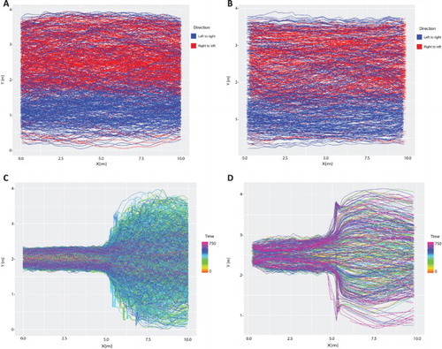
Using the top performing parameter sets shown in Table 2, simulated bidirectional and narrow bottleneck trajectories were obtained. The figure below shows a side-by-side comparison of the trajectories obtained from the experimental data and the trajectories obtained from the simulation.

Figure 2 presents a trajectory comparison between experimental data gathered by TU Delft and the corresponding trajectories that were gathered from the IM model. From the top, the images show: Bidirectional Flow (Left to right in blue and right to left in red) [A, B] and Narrow Bottleneck [C, D]. In the two directional flow situation, in addition to matching in terms of area occupied by pedestrians (i.e. area mainly occupied by pedestrians moving from right to left –red trajectories – versus area occupied mainly by pedestrians moving from left to right – blue trajectories), the simulation suggests lane formation similar to that seen in the data, although this phenomenon cannot be definitively observed with all of the trajectories plotted at once. In the simulated bottleneck result, the funneling effect can be seen as the pedestrians fan outwards before entering the bottleneck area. The experimental and simulated results from the narrow bottleneck show relatively sharp zig-zagging trajectories from pedestrians traveling on the outermost edge of the funnel shape who are attempting to enter the central area.

Figure 2. Observed (left) and the simulated (right) trajectories.

The next section describes the numerical results gathered from simulation, including a comparison of the flow–density diagrams obtained from the data and from the simulation of the bidirectional flow and narrow bottleneck scenarios. Using the calibrated parameters shown above, a transit station scenario was simulated. The results from the transit simulation are also shown in the following section.

4. Simulation

In addition to measuring the distance between the experimental and the simulated trajectories, the flow–density relationships were also analyzed. The figure below shows the flow–density diagrams obtained from the data as well as the flow–density diagrams obtained from the simulation for the bidirectional flow scenarios. The flows and densities of the simulations were recorded from the trajectories that were obtained using the previously described optimal parameter sets for each scenario. The flow was measured by recording the time at which a pedestrian crossed a specified point in the scenario. These times were then aggregated to correspond to a single, full second. For example, pedestrians crossing the specified meter mark at 3.5, 3.7, and 3.9 seconds were all included in the flow count at 3 seconds. The measured flow was divided by the observed width of the walking area in order to come up with a pedestrians/meter/second value. The density measurement was conducted in various ways, including the Fruin method and the XT-method. However, it was found that extrapolating the density from the pedestrians’ speed was favorable since it was not affected by the need to select a specific grid size, as is required by both the Fruin and XT-method.

Figure 3 shows that the simulated flow–density diagrams achieved similar shapes and values to those created from the experimental data for the bidirectional flow scenario. However, it can be seen that no congestion has been observed in both the experimental and the simulation results; moreover, the simulated bidirectional flow density had more frequent observations near the upper part of the diagram in addition to slightly higher observed density.

Figure 3. (A) Bidirectional flow–density diagram from experimental data and (B) bidirectional flow–density diagram from simulation.

As for the simulated bottleneck scenario results, the authors clearly observe a capacity reach at a flow of around 2.5 pedestrian/second/meter in the area directly at the entrance of the bottleneck. The corresponding flow–density diagram is presented in Figure 4.

Figure 4. Narrow bottleneck flow–density diagram from simulation.

The simulated narrow bottleneck flow density closely matched the reported numbers from Zhang et al. (2011). However, the experimental data resulted in a much wider range of observed densities. It should be noted that the results are promising but the expected triangular shape fundamental diagram is not as elaborate as it was expected.

Using the six IM parameters that resulted in the lowest distance between trajectories, the model was tested on a transit scenario as illustrated in Figure 5. The trajectory data obtained are presented in Figure 6.

Figure 5. Transit station platform illustration.

Figure 6. (A) Trajectories from transit simulation and (B) density plot from transit simulation.

For the simulation of the transit scenario, it was assumed that pedestrians entered the platform from the escalator near the right section of Figure 5(A) as well as from train doors. Pedestrians were able to leave the platform via the more centrally located escalator as well as by entering train doors. Pedestrians arriving onto the platform and moving toward train doors were initialized using the optimal parameter set from the bidirectional flow scenarios, while pedestrians exiting the platform (i.e. moving from the train doors to the centrally located escalator) were initialized using the optimal parameter set from the narrow bottleneck scenario. These initialization decisions were made because pedestrians coming onto the platform were more likely to experience bidirectional flow situations than narrow bottleneck situations, while the pedestrians attempting to leave the platform via the escalator were almost inevitably going to experience a narrow bottleneck situation. In order to generate the input data for the pedestrians in the transit simulation, a variety of variables were selected. Initially, each pedestrian was assigned a walking direction determining whether the pedestrian would be entering or exiting the platform. The walking direction of the pedestrian influenced all other initialization variables including start time, starting coordinates, and desired destination. For pedestrians entering the platform from the escalator, a random start time between 0.1 and the desired runtime of the simulation was chosen. Starting coordinates for these pedestrians were limited to the location of the escalator (labeled as ‘down’ in Figure 5). These pedestrians had a 90% chance of aiming for a hotspot on the platform (i.e. a position in which they would be near the arriving train’s doors). The pedestrians aiming for hotspots randomly selected one of the 12 available train door hotspots (6 on each side of the platform) as their destination. Pedestrians entering the platform from trains were given start times corresponding with the arrival of trains, which occurred every 3 minutes. These pedestrians were randomly assigned to start at 1 of the 12 available train doors. The desired destination of all pedestrians exiting the platform was the centrally located escalator (labeled ‘up’ in Figure 4). The transit simulation was conducted using this input information as well as the previously described parameter sets. The resulting trajectories as well as a density plot of the transit platform are shown in Figure 6. Figure 6(B) shows the density at each x-coordinate in the transit station, showing the highest densities corresponding to the area in near the entrance of the centrally located escalator. Figure 6(A) shows that the high densities near the entrance of the centrally located escalator (as confirmed by Figure 6(B)) resulted in the formation of a small bottleneck.

5. Conclusions and recommendations

Pedestrian modeling faces numerous challenges, ranging from covering heterogeneity among the behavior of individuals to a lack of commonly used datasets. These difficulties affect models in different ways – the heterogeneity of pedestrians contributes to the nonexistence of a single model that can accurately describe all types of scenarios, and the lack of common data sets contributes to different approaches taken by authors to validate their models. Furthermore, there is a lack of commonly accepted calibration and validation methods as well as a lack of agreement on which phenomena and behaviors a model should be able to capture, which adds to the difficulty of verifying that a particular model is working well. Although the pedestrian modelers’ ultimate goal, of being able to realistically simulate all types of situations with a single model, has not yet been reached, there are many models which are capable of reproducing specific situations. The IM approach is intended to be used in high density situations, and this paper discusses the initial calibration and validation efforts that have been taken toward achieving that goal. In order to further improve this model, experimental data gathered in high density situations will need to be used for calibration. Additionally, a sensitivity analysis must be conducted, in addition to more intensive calibration efforts, in order to verify that the IM approach is capable of simulating all types of scenarios that are seen in transit stations. Future calibration efforts will consist of a thorough macroscopic and microscopic calibration in addition to specifying more individualized pedestrian information. Based on the testing described above, it appears that pedestrian modeling may benefit from considering numerous obstacles/pedestrians in the vicinity of the pedestrian under consideration, as opposed to the classic approach of considering only a single other entity. The primary future goal identified by the authors of this paper is to collect data from high density experiments, which will be invaluable to this model, as well as to other models with similar objectives.

Disclosure statement

No potential conflict of interest was reported by the authors.

References

- Antonini, Gianluca, Michel Bierlaire, and Mats Weber. 2006. “Discrete Choice Models of Pedestrian Walking Behavior.” Transportation Research Part B: Methodological 40 (8): 667–687. doi: 10.1016/j.trb.2005.09.006
- Blue, V. J., M. J. Embrechts, and J. L. Adler. 1997. “Cellular Automata Modeling of Pedestrian Movements.” Paper presented at the 1997 IEEE international conference on systems, man, and cybernetics, 1997. Computational cybernetics and simulation, Vol. 3, IEEE, 2320–2323.
- Crociani, L., and G. Lämmel. 2016. “Multidestination Pedestrian Flows in Equilibrium: A Cellular Automaton-Based Approach.” Computer-Aided Civil and Infrastructure Engineering 31 (6): 432–448. doi: 10.1111/mice.12209
- Daamen, Winnie. 2004. Modelling Passenger Flows in Public Transport Facilities. TU Delft: Delft University of Technology.
- Daamen, W., and S. P. Hoogendoorn. 2003. “Experimental Research of Pedestrian Walking Behavior.” Transportation Research Record: Journal of the Transportation Research Board 1828: 20–30. doi: 10.3141/1828-03
- District of Columbia Department of Transportation. “District of Columbia Pedestrian Master Plan.” Technical Report. Accessed 10 January 2015. http://ddot.dc.gov/sites/default/files/dc/sites/ddot/publication/attachments/pedestrianmasterplan_2009.pdf
- Duives, Dorine C., W. Daamen, and S. P. Hoogendoorn. 2013. “State-of-the-Art Crowd Motion Simulation Models.” Transportation Research Part C: Emerging Technologies 37: 193–209. doi: 10.1016/j.trc.2013.02.005
- Flötteröd, G., and G. Lämmel. 2015. “Bidirectional Pedestrian Fundamental Diagram.” Transportation Research Part B: Methodological 71: 194–212. doi: 10.1016/j.trb.2014.11.001
- Gniewek, Pawel, Sumudu P. Leelananda, Andrzej Kolinski, Robert L. Jernigan, and Andrzej Kloczkowski. 2011. “Multibody Coarse-Grained Potentials for Native Structure Recognition and Quality Assessment of Protein Models.” Proteins: Structure, Function, and Bioinformatics 79 (6): 1923–1929. doi: 10.1002/prot.23015
- Hänseler, F., B. Farooq, T. Muhlematter, and M. Bierlair. 2013. “An Aggregated Dynamic Flow Model for Pedestrian Movement in Railway Stations.” Paper presented at the proceedings of the 13th Swiss transport research conference, April 24–26, 1–14.
- Helbing, Dirk, Lubos Buzna, Anders Johansson, and Torsten Werner. 2005. “Self-Organized Pedestrian Crowd Dynamics: Experiments, Simulations, and Design Solutions.” Transportation Science 39 (1): 1–24. doi: 10.1287/trsc.1040.0108
- Helbing, D., and P. Molnár. 1995. “Social Force Model for Pedestrian Dynamics.” Physical Review E 51 (5): 4282–4286. doi: 10.1103/PhysRevE.51.4282
- Hoogendoorn, S. P., and W. Daamen. 2005. “Pedestrian Behavior at Bottlenecks.” Transportation Science 39: 147–159. doi: 10.1287/trsc.1040.0102
- Jian, Xiao-Xia, S. C. Wong, P. Zhang, K. Choi, H. Li, and X. Zhang. 2014. “Perceived Cost Potential Field Cellular Automata Model with an Aggregated Force Field for Pedestrian Dynamics.” Transportation Research Part C: Emerging Technologies 42: 200–210. doi: 10.1016/j.trc.2014.01.018
- Johansson, Anders. 2004. “Pedestrian Simulations with the Social Force Model.” Master thesis.
- Johansson, Anders, Dirk Helbing, Habib Z. Al-Abideen, and Salim Al-Bosta. 2008. “From Crowd Dynamics to Crowd Safety: A Video-Based Analysis.” Advances in Complex Systems 11 (4): 497–527. doi: 10.1142/S0219525908001854
- Johansson, Anders, Dirk Helbing, and Pradyumn K. Shukla. 2007. “Specification of the Social Force Pedestrian Model by Evolutionary Adjustment to Video Tracking Data.” Advances in Complex Systems 10 (Suppl. 2): 271–288. doi: 10.1142/S0219525907001355
- Ko, M., T. Kim, and K. Sohn. 2013. “Calibrating a Social-Force-Based Pedestrian Walking Model Based on Maximum Likelihood Estimation.” Transportation 40 (1): 91–107. doi: 10.1007/s11116-012-9411-z
- Lehmann, Erich Leo, and George Casella. 1998. Theory of Point Estimation. Vol. 31. New York: Springer Science & Business Media.
- Moussaïd, M., D. Helbing, and G. Theraulaz. 2011. “How Simple Rules Determine Pedestrian Behavior and Crowd Disasters.” Proceedings of the National Academy of Sciences of the United States of America 108 (17): 6884–6888. doi: 10.1073/pnas.1016507108
- Paris, Sébastien, Julien Pettré, and Stéphane Donikian. 2007. “Pedestrian Reactive Navigation for Crowd Simulation: A Predictive Approach.” Computer Graphics Forum 26(3): 665–674.
- Tao, Wang, and C. Jun. 2009. “An Improved Cellular Automaton Model for Urban Walkway Bi-Directional Pedestrian Flow.” Paper presented at the international conference on measuring technology and mechatronics automation, 2009 (ICMTMA’09), Vol. 3, IEEE, April 11–12, 459–461.
- Van Den Berg, J., S. J. Guy, M. Lin, and D. Manocha. 2011. “Reciprocal n-Body Collision Avoidance.” In Robotics Research: The 14th International Symposium ISRR, Springer Tracts in Advanced Robotics, vol. 70, edited by C. Pradalier, R. Siegwart, and G. Hirzinger. Lucerne: Springer-Verlag, 3–19.
- Zanlungo, F., T. Ikeda, and T. Kanda. 2011. “Social Force Model with Explicit Collision Prediction.” Europhysics Letters Association EPL (Europhysics Letters), 93 (6): 68005. doi: 10.1209/0295-5075/93/68005
- Zhang, J., W. Klingsch, A. Schadschneider, and A. Seyfried. 2011. “Transitions in Pedestrian Fundamental Diagrams of Straight Corridors and T-Junctions.” Journal of Statistical Mechanics-Theory and Experiment 2011: P06004.
- Zhang, R., L. Zhihong, J. Hong, D. Han, and L. Zhao. 2009. “Research on Characteristics of Pedestrian Traffic and Simulation in the Underground Transfer Hub in Beijing.” Paper presented at the fourth international conference on Computer Sciences and Convergence Information Technology, 2009 (ICCIT’09), IEEE, November 24–26, 1352–1357.