A method to estimate the capacity of an intersection of waterways in ports

Abstract

The maritime transportation growth leads to more intensively used waterways, especially in ports. Since the capacity of an intersection of waterways becomes more important, this research presents a new method to estimate this capacity. Based on an analogy between roads and waterways, the conflict technique is applied to an intersection of waterways. The vessel flows in each direction and their conflicting movements are input for the capacity calculation. The generic method can be applied to any intersection, considering the conflicts between the different streams in the intersection and the flows inferred from empirical data or from predictions. The applicability of the method is shown with two case studies, based on data from the Port of Rotterdam. After using the proposed method, we compare the real flows with the estimated ones to assess the capacity estimates. This method can improve traffic management strategies, traffic rules in waterway intersections or port designs.

KEYWORDS:

• Capacity
• waterway intersection
• maritime traffic
• AIS data
• radar data

1. Introduction

Maritime transportation is continuously growing and waterways have to handle higher traffic flows. As a result, waterway intersections are more intensively used and more crowded for navigation. Since port authorities are concerned about the maximum vessel flow that intersections can accommodate, the main question in this research is: ‘How can we determine the capacity of an intersection of waterways?’.

Capacity has been a subject of interest in maritime transportation research, but usually more focused on the terminal level rather than on the wet infrastructure level. Recent research has focused on the effects of high vessel flows in ports with different purposes. A recent practical study presented the application of domain analysis to a port area to assess navigational risks (Rawson et al. 2014). Similar research was developed for seaport fairway capacity by (Wang et al. 2015), while analyzing different port safety and service levels. Another application of ship domain was done to analyse the free flow efficiency of vessel traffic between two pilons while including a Traffic Separation Scheme (TSS) (Jensen et al. 2013). Liu et al. (2016) developed a ship domain model, based on trigonometrical relations for capacity analysis of waterways. Their approach includes crossings in navigations, but the different turning directions within an intersection are not included. At an aggregate level, a method to estimate the capacity of a port network, using a simulation model, has been recently presented (Bellsolà Olba et al. 2017). Even though the capacity of waterways and fairways or port networks has been already extensively addressed, an method to estimate the capacity value of an intersection of waterways in ports have not been specifically developed. The previous methods allow the calculation of the current capacity and it can be compared to a service level, but how to determine objectively a maximum value has not been performed. Because of this, we aim to fullfil this gap with this research.

The definition of capacity of a waterway intersection has not been previously formulated. The definition may be similar to the definition for approach channels (McBride, Boll, and Briggs 2014): ‘the maximum traffic volume to be handled by the approach system satisfying the required service level and safety level’. This definition considers an approach system instead of a waterway intersection, and the vessel composition and traffic shares (OD matrix) are not included. The vessel composition and the traffic shares have a direct effect on capacity, and it will be lower with larger vessels or when vessels have specific encountering safety requirements. Correspondingly, we propose the following definition for the capacity of a waterway intersection: ‘the maximum traffic volume to be handled by an intersection of waterways satisfying the required safety level, and conditional on the traffic composition and traffic shares over different directions’. The utilization of the intersection can be considered as the number of vessels passing the intersection through cross-sections in each direction during a certain time interval. Thus, the difference between the estimated capacity and the utilization is a proxy for assessing the current traffic situation, as it allows to find out if there is still space for the port to grow or if new port designs or other traffic management strategies should be implemented to avoid a bottleneck in a specific intersection.

The capacity estimation of vessel traffic in intersections of waterways is difficult due to the uncertainty in vessel arrivals, which has been shown to be random (Fararoui 1989; Pachakis and Kiremidjian 2003), and the different traffic shares, which vary over time as well. A good estimate of the capacity of an intersection of waterways could be obtained using a port simulation model, but a method to estimate its capacity does not yet exist. The objective of this research is to develop a generic method to estimate the capacity of any waterway intersection on a high level. The method is suitable for and applicable by any stakeholder to compare the current situation with the estimated capacity. Since a similar method has not been previously developed, research in other fields is considered. This paper continues with the review of existing capacity estimation methods for roads and their characteristics (Section 2). Based on the literature review, an analogy between waterways and unsignalised intersections in roads can be drawn because of their similarities. Based on this analogy, a capacity estimation method for waterway intersections is developed (Section 3). Section 4 presents two case studies where a data analysis is performed and the method is applied to two different intersections. This case study describes the data used, which leads to the input for the method, followed by the capacity calculations and a sensitivity analysis. The last section presents the summary and future research (Section 5).

2. Background

Waterway intersections have many similarities with unsignalised road intersections, such as certain headway between vessels and different choice of directions, but also important differences, such as communication among vessels and between vessels and the port, with the Vessel Traffic Services (VTS), exist. Moreover, there are no queues at intersections, to indicate that the capacity has been reached.

Though a method to estimate the capacity of waterway intersections does not exist, the concept of estimating intersection capacity has been extensively studied for road traffic. Previous research on unsignalised road intersections presented two methods to estimate capacity: the gap-acceptance theory (among others, Brilon, Koening, and Troutbeck 1999; Amin and Maurya 2015), and the conflict technique (Brilon and Miltner 2005).

The first method is based on the idea of estimating the minimum critical gap, which is the minimum headway during which each individual driver will accept to enter the intersection. This critical gap is different for each individual, resulting in a critical gap distribution. In unsignalised crossings, the driver of the vehicle without priority will accept a gap between vehicles in the main stream to enter the intersection if the offered gap is larger than his/her critical gap. This critical gap can be estimated with different methodologies, such as the maximum likelihood or Hewitt's method (Brilon, Koening, and Troutbeck 1999). The value or distribution for the critical gap, estimated with any of the existing methods, can be used to determine the capacity of the intersection. However, the critical gap estimation method has some drawbacks, as stated by Brilon and Wu (2001). For example, the critical gap estimated is different depending on the direction of the vehicle, and requires a clear definition of traffic rules, which hampers its use for the estimation of a single capacity value for other transport modes. There are many rules in waterways which are based on the sailors code of conduct and the local port regulations and, since each combination is unique, it is difficult to come up with a generic definition.

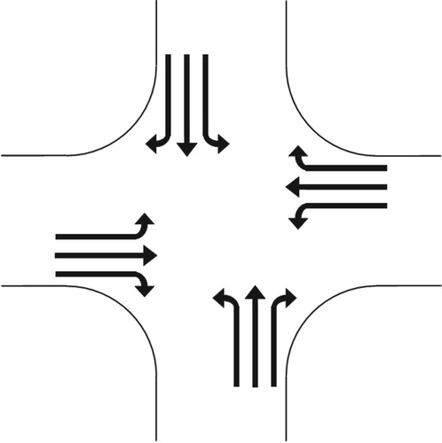
The second method, the conflict technique, simplifies the movements and operations of an intersection representing the intersection as a queuing system (Brilon and Miltner 2005). For the intersection capacity calculation, they consider the flows in each stream and the interactions between them. Road users, from both traffic streams, will occupy the conflict area. This area is the space in the intersection that cannot be used simultaneously by vehicles from different streams. Road users from the major stream can pass the intersection, while the ones from the minor stream must wait when the conflict area is occupied. The probability that the intersection is blocked can be calculated for each stream by multiplying the traffic flow and the time that a vehicle occupies the intersection. As a road user could enter the intersection when the conflicting streams are free of traffic, the capacity for each movement is calculated as the probability that the conflict area is not occupied times the probability that no other vehicle is coming during a specific time interval. A total of 28 movements are allowed at a 4-way intersection with two-way traffic, including the movements of cyclists, pedestrians and vehicles. However, in case of just considering the cars, a total of 12 movements would be allowed (see Figure 1). The more streams in an intersection, the more conflicts will occur between the different streams.

Figure 1. Definition of traffic movements at an intersection of waterways.

3. Capacity estimation method for waterway intersections

The gap-acceptance theory is not suitable for our purposes because vessel traffic flows are not constant and do not have high densities for long periods of time. In addition, since vessel communication and decision making are different from road traffic when approaching an intersection, the gaps could not be estimated using a similar method.

As a starting point to develop a capacity estimation method for waterway intersections, we therefore consider the conflict technique. This technique considers the intersection as a queueing system with probabilities of conflict between different streams from the traffic flow shares in each stream. This method has the drawback of simplifying the intersection into a queuing system which does not respect the complexity of reality. However, a generic method which includes all the specificities of waterway intersections is not feasible, and it might not provide great differences compared to a simplified one on an aggregated level. The advantage of the method presented is that it allows the estimation of the capacity with the consideration of traffic shares and the time vehicles are blocking the intersection. Hence, we consider that a capacity estimation method for waterway intersections can be derived from the conflict technique method.

There are similarities and differences between roads and waterways, and the relevant ones need to be described. The total number of possible vessel movements in a waterway is 12, as shown in Figure 1. These movements are the same as for vehicles on roads, excluding cyclists and pedestrians. With respect to priorities, waterways do not have right-of-way priority, vessels communicate amongst each other and the VTS provides information and navigational advice to support their navigation, always under navigators responsibility. Apart from this, each crossing may have specific priorities according to some vessel types or sizes, the waterway design and dedicated port regulations, such as Traffic Separation Schemes (TSS), where vessels have idependent sailing lanes. Otherwise, vessels navigators behaviour should satisfy to COLREGs (COLREG 1972) and common practices. For example, LNG tankers might not be allowed to cross with other vessels, so the intersection should be completely blocked for other vessels while these tankers are crossing. One more difference is related to the flow. During the peak times, the stochastic vehicle arrival at a road intersection might have less variation than the vessel arrival in waterways.

The input required by the conflict technique is the total vehicle flow, the occupation duration of the intersection and the traffic share for each direction. Based on the specificities in waterways, as done in road traffic, some assumptions are made in order to turn the conflict technique into an applicable method for waterways. First, although a large variety of vessel types exists, no difference in vessel types and sailing speeds are considered. There are faster and slower vessels, as cars and other vehicles on roads, but they can be respresented with an average value when looking into an aggregated level. As explained before, the navigation is assisted by VTS and there might be specific priorities for some vessel types that limit the traffic because dangerous encounters, which might lead to a reduced capacity. In this research, we aim to find a maximum value, so the assumption is useful for high-level calculations where the value is used for strategic or tactical assessment of navigational or infrastructure changes. Second, the occupation time of the intersection will be averaged according to the speed used, as previously used in the method for unsignalised road intersections (Brilon and Wu 2001). Last, we consider that, with a high traffic flow, VTS control might have stronger influence which leads to dependent arrivals. Hence, the vessel arrival is assumed to be uniform over time.

Since the waterways are usually not sufficiently congested, it is difficult to estimate a minimum headway between vessels. This minimum headway could be estimated from data when having reliable data available. In this research, we use a theoretical minimum safe time clearance kept by each vessel with respect to its predecessor, and we name it as safe headway ($h^{\text{safe}}$ [s]). Previous studies considered the safe vessel braking distance (d_n [m]) in confined waters as 3 times the vessel length (Fujii and Tanaka 1971; Pietrzykowski 2008), independent of vessel speed and load of the vessel. More recent studies, based on AIS data, have shown that a longitudinal space in front of a vessel suits the comfort zone of ship navigators in open waters (Hansen et al. 2013). Thus, for confined waters, we define the individual safe vessel braking distance (d_n) as 3 times the vessel length. Hence, the safe headway for each individual vessel ($h_n^{\text{safe}}$) can be calculated as d_n divided by its speed over ground (v_n [m/s]) in the direction towards the intersection (speed measured on surface, while the vessel might navigate at a higher or lower speed depending on the current in the water), as shown in the following equation: (1) $h_n^{\text{safe}}=\frac{d_n}{v_n}$(1)

In vehicular traffic, it is assumed that while a vehicle is occupying the area of conflict, no other vehicle can enter until the first vehicle leaves the area of conflict. For waterways, due to the larger distance to cover and the low sailing speed, two conflicting vessels could be allowed simultaneously at the intersection. Hence, we consider that when the vessel inside the intersection has travelled more than half of the length of her path through the intersection to her specific direction, the next vessel can safely enter the intersection area, always respecting d_n.

The mean safe headway (${\overline{h}}^{\text{safe}}$) can be calculated as the mean of $h_n^{\text{safe}}$. Since this is dependent on data availability, in case of not having this individual speed data, an educated estimation of the mean speed, for example, in relation to waterway limits (width and water depth), can be made by expert consultation. In case of a large vessel, the mean safe headway might be larger than the length of the area of conflict, thus only one ship could enter the intersection.

Equation (2) introduces the maximum flow in any stream without any conflict (q_1D [vessels/hour]), which can be calculated with the inverse of ${\overline{h}}^{\text{safe}}$ ([h]). As a result, the calculated flow is the total number of vessels that is able to cross the intersection within an hour in any direction without any conflict with other directions. (2) $q_{1D}=\frac{1}{{\overline{h}}^{\text{safe}}}$(2)

The probability that a vessel from stream i occupies the intersection (P_i) can be obtained by multiplying three factors (see Equation (3)). The first factor (${\alpha }_i$) is the percentage of traffic volume from an origin to a destination. If vessels are considered to sail simultaneously from the same origin towards different destinations, because of the existence of TSS with exclusive lanes for each direction, this factor would be one. When there is no TSS in the area, ${\alpha }_i$ represents the share of traffic going to each direction. The second factor is the maximum flow in one direction without any constraint ($q_{1D}$), previously defined, and the third one is the occupation time (δ_i). δ_i represents the time that a vessel occupies the intersection, and it is obtained by dividing the sum of the path that follows the direction of stream i and the vessel length, as the conflicting distance previously discussed, by the average speed over ground of all vessels. The conflicting distances are defined for each combination of origin and destination at the intersection. After a vessel has travelled the corresponding conflicting distance, the conflict area is free and a coming vessel from any direction is allowed to enter the intersection. (3) $P_i={\alpha }_i\cdot q_{1D}\cdot {\delta }_i$(3)

A conflict matrix (A), which identifies all movements that cannot occupy the area simultaneously, is used to define whether a conflict occurs between two streams (0 if no conflict occurs or 1 if a conflict occurs). The conflicts are defined considering two opposite streams as free of conflicts, while the rest of directions will have conflicts with these free streams. Then, the probability of conflict of each stream (P_c,i) is defined in Equation (4). To calculate it, the conflict probability of each stream should be obtained. The probability of occupying the intersection by stream i multiplied by the sum of probabilities that any of the other streams occupies the intersection in case of conflict, and by the conflict factor (A_ij), equals to the probability of occupation from stream i. When there is no conflict, the resulting value is 0. Hence, P_c,i can be calculated as the sum of probabilities of conflict for each of the streams: (4) $P_{c,i}=\sum _i\left(P_i\cdot \sum _{j\ne i}{P}_j\cdot A_{ij}\right)$(4)

Equation (5) defines the capacity of each stream by multiplying the maximum flow for stream i (${\alpha }_i\cdot q_{1D}$) and the probability of not having encounters in stream i, which equals to one minus the probability of having an encounter (P_c,i). The resulting value provides an estimated value of the maximum vessel flow of each stream. (5) $C_i={\alpha }_i\cdot q_{1D}\cdot \left(1-P_{c,i}\right)$(5)

The value of C for the whole intersection is obtained with the sum of the capacity in each direction by using Equation (6). (6) $C=\sum C_i$(6)

4. Case study

The application of the estimation method in a real scenario is used to demonstrate its applicability. Therefore two case studies of intersections from the Port of Rotterdam have been carried out. Data from the Automatic Identification System (AIS) and the radar have been used. An explanation of both types of data and what is included in both datasets is presented in the Subsection 4.1. The following subsections present the research area and the content of the dataset (Subsection 4.2), the analysis of the datasets used (Subsection 4.3), the results of the capacity estimation (Subsection 4.4) and a evaluation of the method (Subsection 4.5). To investigate the effect of the input variables from the method, a sensitivity analysis is performed in Subsection 4.6.

4.1. Automatic identification system (AIS) and radar data background

Since we want to apply the method previously developed in a real waterway intersection, we use data from two different vessel traffic recording systems.

The Automatic Identification System (AIS) was established by The International Association of Marine Aids to Navigation and Lighthouse Authorities (IALA). AIS is an autonomous and continuous broadcast system, that operates in the Very High Frequency (VHF) maritime mobile band (IALA 2004). The principal functions of AIS, indicated by IALA (2004), are: (1) the information exchange between vessels within VHF range of each other to increase the situational awareness and safety; (2) the information exchange between a vessel and a shore station, such as a Vessel Traffic Service (VTS), to improve traffic management in congested waterways; and (3) the automatic location reporting in areas of mandatory and voluntary reporting. The shipboard information from the vessel sensors includes static, dynamic and voyage related data.

Similar data can be obtained with radars; they are obtained from the reflection of short pulses of radio waves generated by the radar that are reflected back by the vessels. The distance between the vessel and the radar can be obtained (Sonnenberg 2013).

There are advantages and disadvantages for both AIS and the radar datasets to be applied in this case study (Lin and Huang 2006). The coverage for AIS is around 40 nautical miles, while for the radar coverage is limited to 24 nautical miles, even though different radar coverages can be fused. Regarding the vessel position, although the AIS and the radar data have some differences in the dynamic variables (speed, latitude, longitude, etc.), their accuracy is similar (Lin and Huang 2006). In specific cases there are large differences that might be due to problems with the AIS or the radar signals.

Radar coverage might be limited in space due to radar blind and shadow areas, and some areas might be uncovered. If this happens, it can be identified. Moreover, all vessels are visible under the radar coverage, while in AIS data, only vessels with AIS transmitters are visible. Since 2000, the requirements have been changing and, nowadays, most of the cargo and passenger vessels need to have a transmitter installed (International Maritime Organization 2000). Since just part of the inland vessels have an AIS transmitter, and almost none of the recreational ones, the radar coverage is normally better than the AIS inside a port.

Both AIS and radar data have several practical applications, such as collision avoidance, vessel traffic services (VTS), maritime security, aids to navigation, search and rescue and accident investigation (Yip 2008; Kujala et al. 2009; Mou, van der Tak, and Ligteringen 2010; Tsou 2010). The use of AIS and radar data for research provides the opportunity to develop statistical analysis of accidents, vessel behaviour, etc., taking into account different circumstances, including weather, time of the day or year, among other things. The relevant information included in the AIS and radar messages for this research is summarized in Table 1. As it can be seen, there are few differences in content between AIS and radar datasets, but these differences do not affect the application of the method and the required inputs are available in both datasets. One main difference between the two datasets is the signal identification. The AIS signals are recorded based on the MMSI, which is a unique number for each vessel and allows to follow their path with the consecutive signals. Although, the radar data records signals without any information for the identification of which vessel is it, the dataset used has already a track number that identifies each vessel trip with a unique number. Recent studies have shown the possibility of using data fusion algorithms to combine the both datasets, which might allow the detection of errors in the AIS data among others (Kazimierski and Stateczny 2015).

Table 1. AIS and radar information.

Information	AIS	Radar
MMSI number	X
Length [m]	X	X
Beam [m]	X	X
Longitude (X coord.)	X	X
Latitude (Y coord.)	X	X
Speed	X	X
Heading	X	X
Course over ground	X	X
Draught	X
Date/Time	X	X
Vessel type	X	X
Track number		X

4.2. Research area and dataset

The estimation method introduced has been tested in two intersections in the Port of Rotterdam (the Netherlands) shown in Figure 2. The research areas considered are two T junctions between two waterways, Oude Maas–Hartelkanaal (see plain square in Figure 2), and Oude Maas–Nieuwe Maas (see striped square in Figure 2). The chosen intersections are ones of the busiest intersections in the Port of Rotterdam, and the intersections do not have a TSS scheme. The datasets for this research were provided by the Port of Rotterdam Authority.

Figure 2. Research areas in the Port of Rotterdam (Oude Maas–Nieuwe Maas intersection (striped square) and Oude Maas–Hartelkanaal (plain square)).

The first dataset used is from the Oude Maas–Hartelkanaal intersection (I1), and it contains the information of a week of both AIS and radar data, from the 1st until the 7th of September 2014. The daily patterns in vessel traffic have been derived by investigating a week of data. The weather conditions during that week were favourable, which do not have any implication on the vessel behaviour from the dataset.

The Port of Rotterdam has radar stations all along their waterways covering the complete area, with some areas with lower radar effectiveness. However, as previously introduced, not all inland vessels are AIS-equipped. In this research, in case of just using the AIS information, the total amount of vessels would be underestimated. The dataset contains all the signals from vessels using radar data, but only 62% of these signals have AIS details. For this reason, the radar data have been used for the analysis.

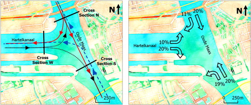
Figure 3 shows a detailed layout of I1 with some vessel trajectories. Although vessels do not follow specific lanes, and there is no a TSS scheme for this intersection, they tend to sail along similar paths. In the research area, based on the density analysis of the dataset, the paths are defined more or less by two separated directions in each waterway (see Figure 4, left), except for the north part of the Oude Maas, due to an infrastructure constraint. In that location there is a bridge crossing the waterway, thus vessels need to adjust their path between the piles of the bridge. The width between the piles is large enough not to affect vessel navigation when encountering other vessels in this area. The intersection area chosen for the calculation is the area between each of the cross-sections defined in Figure 4 (left).

Figure 3. Example of vessel trajectories in the Oude Maas–Hartelkanaal intersection (I1).

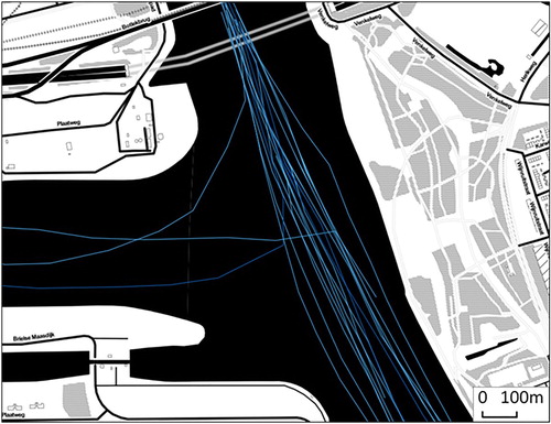
Figure 4. Oude Maas–Hartelkanaal map (vessel paths (left) and traffic shares (right)).

The minimum interval between consecutive signals from a vessel is 5 s, and the dataset has almost half a million messages recorded from 5209 different vessels. Each signal consists of a coordinate point in the area and the tracks are obtained by linking all the points that belong to the same track for each vessel. Each of these tracks is a vessel passing the intersection, which means that repeated visits from the same vessel count as independent tracks.

The moored vessels, mainly in the north side of the Hartelkanaal, keep also sending signals every 1–3 min. This means that from the whole dataset, almost 70% of the messages are from moored vessels, which are removed from the dataset as they do not occupy space in the intersection, and as such, these are not relevant for the capacity estimation. Hence, there are 3395 individual sailing vessel tracks remaining. From the remaining individual vessel tracks, only 66% have a whole track going from one of the cross-sections of the intersection to another one (see Figure 4, right). Most of the partial tracks consist of few signals next to the berthing areas, which are assumed to be moored vessels, and these vessels do not affect to the vessel traffic in the intersection. The remaining signals are partial tracks with few signals which do not provide enough information for their analysis. These might be erroneous recordings with missing data or signals from vessels moored which coordinates are wrong. Many of these signals have a time interval longer than expected for a sailing vessel to cross the intersection. In this research, we assume that the distribution of wrong signals is equal in all directions, thus, it does not have an effect on the traffic shares in each direction. Therefore, the estimation method is not affected by their removal.

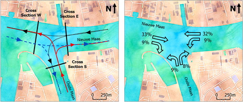
The second dataset is from the Oude Maas–Nieuwe Maas intersection (I2). This dataset is more limited and it contains the passing vessel information from three cross-sections in that intersection (see Figure 5). This dataset contains the information of a week of radar data during a busy week from 2015, from the 9th until the 15th of May. This dataset contains a total of 8192 recordings, which correspond to a total of 3745 vessel identified vessel tracks that go from a cross-section to another one. The rest of the signals (around 9%) are unidentified vessels which cannot be tracked.

Figure 5. Oude Maas–Nieuwe Maas map (vessel paths (left) and traffic shares (right)).

4.3. Data analysis

Once the datasets have been cleaned, the resulting information has been analysed and used to evaluate the applicability of the estimation method presented in Section 3.

The estimation method considers the assumption of an average speed for all vessels to calculate the occupation time in the intersection. A first hypothesis is that a correlation between vessel dimensions and sailing speed exists for vessels in a port. However, as shown in Table 2, the data analysis for I1 revealed a low correlation between the length or the beam of the vessels and their speed. This could be explained because ships are sailing within a limited speed range due to port regulations. So, even though vessels might be able to sail faster, in some cases, they maintain a lower speed. Thus, the assumption of an average speed for all vessel types holds for the application of the method. Regarding the correlation between vessel speed and headway (passing time interval with respect to the predecessor vessel), the dataset does not reflect any pattern between them due to the stochastic traffic flow during the day. Hence, we do not consider any possible correlation in this research.

Table 2. Correlation values between variables for I1.

Variables	Speed
Length	−0.32
Beam	−0.31
Headway	−0.07

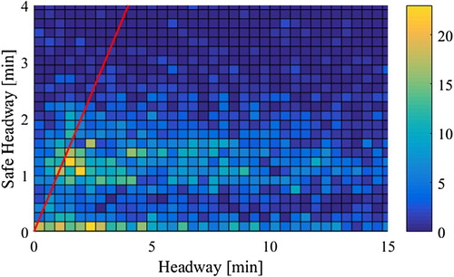
In order to apply the method, the first step is to obtain the safe headway for each vessel ($h_n^{\text{safe}}$), which is calculated from each vessel length. We expect the safe headways to be lower than the real hedways (h_n). As shown in Figure 6, it can be seen with a density plot that more than 95% of h_n are higher than $h_n^{\text{safe}}$, and most of the lower ones occur due to overtaking situations or incorrect data that cannot be verified. In reality, vessels maintain always safe distances as shown in previous studies (Pietrzykowski 2008). Based on this, the authors consider h_s to be a suitable approximation of the minimum headway to calculate the vessel flow. The figure shows two main clusters of results. Since $h_n^{\text{safe}}$ is obtained based on d_n, dependent on the vessel length, these clusters might happen because of the most representative vessel lengths.

Figure 6. Density plot of safe headway vs actual headway in I1.

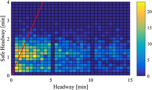
Similar results are obtained for I2, where more than 93% of h_n are higher than $h_n^{\text{safe}}$ (see Figure 7). The time in this dataset is rounded to minutes. Because of this, the headway values in two columns are 0, and the results show a similar pattern as in the previous dataset.

Figure 7. Density plot of safe headway vs actual headway in I2.

The method assumes a unique speed for all vessels to calculate $h_n^{\text{safe}}$. As shown in Table 2, there is little correlation between speed and vessel characteristics. The data showed that vessels with the same characteristics do not keep a specific range of speeds and any vessel type can have low and high speeds. Hence, based on the average speed results from the datasets (see Figures 8 and 9), a vessel speed of 8 knots for I1 and 9 knots for I2 are used to calculate ${\overline{h}}^{\text{safe}}$. For I1, with an average vessel length of 120 m, ${\overline{h}}^{\text{safe}}$ equals to 1.46 min. By using ${\overline{h}}^{\text{safe}}$ in Equation (2), q_1D equals 123.5 vessels per hour (ves/h). For I2, with the same average vessel length, the ${\overline{h}}^{\text{safe}}$ equals to 1.30 min, and q_1D equals 138.9 vessels per hour (ves/h). These values are based on the assumption of uniformly distributed vessel arrivals, but in reality the arrival is not uniform and uncontrolled. When having dense traffic situations, the vessel flow might be substantially influenced by the VTS advice. Hence, the vessel arrival distribution could become uniform. The flow is the maximum value that ideally could be obtained with continuous vessel traffic in one stream.

Figure 8. Vessel speeds per hour of the day (I1).

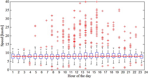
Figure 9. Vessel speeds per hour of the day (I2).

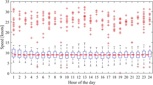
Figure 4, left, shows the possible movements in each direction for I1. Based on these paths, the conflicting movements of vessels in the different directions can be identified. The individual conflicts allow us to build a conflict matrix for the intersection (see Table 3). The table shows, for example, that there is a conflict between vessels going in the direction SW and NS. Thus, their value in the conflict matrix is identified with 1. Table 4 shows the conflicting movements for I2.

Table 3. Conflict matrix I1.

Direction	NS	NW	SN	SW	WN	WS
NS
NW	0
SN	0	0
SW	1	1	0
WN	1	0	1	1
WS	1	0	0	0	0

Table 4. Conflict matrix I2.

Direction	SW	SE	WE	WS	EW	ES
SW
SE	0
WE	1	1
WS	0	0	0
EW	1	0	0	1
ES	1	0	1	1	0

4.4. Results of capacity estimation method

With the results from the data analysis, the calculations to estimate capacity can be performed. First, in order to calculate the probability of conflict per direction, there are several values that need to be defined, and these are summarized in Table 5.

Table 5. Probability of conflict per direction (I1).

Direction	Traffic Share (%)	Distance to cross [m]	${\alpha }_i\cdot q_{1Dx}$ [ves/h]	ti [min]	Pi	1−Pc,i	Ci [ves/h]
NS	20	750	26.7	1.76	0.78	1.00	26.7
NW	11	365	14.5	0.98	0.24	1.00	14.5
SN	20	750	21.5	1.76	0.63	1.00	21.5
SW	19	695	19.7	1.65	0.54	0.45	8.8
WN	10	680	13.3	1.62	0.36	0.30	4.0
WS	20	575	27.8	1.41	0.65	0.49	13.6

The traffic shares for each direction, which can be extracted analysing the different vessel paths from the dataset, are shown in the second column. The time that a vessel from one stream is occupying the intersection (δ_i) is calculated based on the following conditions: the intersection length is defined for each of the directions of each stream, according to Figure 4, left, and the distances vary between a minimum of 365 m up to 750 m; the vessel length is added to the total intersection length for each direction; the distance to be travelled by a conflicting vessel is considered as 50% of these lengths, which leads to a longer distance than 3 times the median vessel length (d_n), as explained in Section 3; and, a speed of 8 knots is used, as explained in the previous subsection.

Considering this occupation time, the different shares per direction and the flows, the probability that each stream occupies the intersection (P_i) is obtained. With this value, conflict probabilities for each direction (P_c,i) are obtained. Using Equation (4), the capacity for each stream is calculated. Hence, the resulting estimated capacity (C) of I1 is the result of the sum of the capacity of each stream, and it equals 89.0 ves/h, considering these specific traffic shares.

When applying the method to the second research area (I2), it can be seen in Table 6, that the traffic shares in this intersection are different. For this intersection, the vessel speed chose is 9 knots, based on the dataset, and with the specific distances for the intersection, the method results on an estimated capacity (C) of 102.8 ves/h.

Table 6. Probability of conflict per direction (I2).

Direction	Traffic Share (%)	Distance to cross [m]	${\alpha }_i\cdot q_{1Dx}$ [ves/h]	ti [min]	Pi	1 − Pc,i	Ci [ves/h]
WE	33	920	36.4	1.43	0.87	1.00	36.4
WS	9	720	9.9	1.30	0.21	1.00	9.9
EW	32	900	36.1	1.39	0.84	1.00	36.1
ES	9	700	10.2	1.11	0.19	0.80	8.1
SW	9	830	24.5	1.28	0.52	0.01	0.1
SE	8	910	21.8	1.41	0.51	0.56	12.1

4.5. Evaluation of the method with real data

In order to assess the capacity estimates calculated with the proposed method, the results can be compared to the maximum observed vessel flow for each intersection from real data. Since usually there are not many traffic peaks in this area due to stochastic arrivals and port regulations, we decided to use a small time interval that allows us to find out significant traffic peaks. Because of this, we decide to use an interval of 6 min (0.1 h).

For I1, the dataset reveals that the maximum number of vessels passing the intersection in this interval has a peak of 7 vessels. The peak of 7 vessels per interval of 6 min can be considered as the capacity value of the intersection. Using this maximum flow, the resulting maximum flow per hour that would cross the intersection is 70 ves/h. From the estimation method, we obtained a value of 89.0 ves/h. This result shows that the intersection has not reached the capacity value, and the maximum flow is around 79% of utilization during peak times. Thus, the intersection could still allocate higher vessel flows.

In the case of I2, for the same interval of time, the maximum number of passing vessels equals to 9. Considering this flow per 6 min interval, the resulting maximum flow crossing the intersection is 90 ves/h. Comparing this result with the estimated capacity of 102.8 ves/h, the utilization during peak times reaches 88%, which is a really high value. A possible explanation for this is because the main flow is from EW and WE (66% as seen in Figure 5, right), which means that the number of conflicts is substantially lower than in I1.

4.6. Sensitivity analysis

This section presents a sensitivity analysis performed to test the effects of various parameters on the estimated capacity in I1. In Figure 10, the estimated capacity of the intersection is drawn against various parameters: safe vessel braking distance (d_n), intersection length and average vessel speed.

Figure 10. Relation between intersection and capacity factor times vessel length (d_n) (top left), % variation of intersection length (top right), and average vessel speed (bottom left).

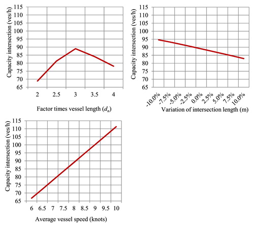
Figure 10, top left, shows that the factor used to calculate d_n provides the maximum capacity for this intersection. The difference between the chosen d_n value and the lower one is 7 ves/h difference. The relevant change appears when d_n reaches 1 or 5. When increasing the distance, the capacity would increase the headways between vessels and, consequently, decrease the flows to around 10 ves/h less for each increase. On the opposite side, when decreasing d_n, many more vessels might be sailing and blocking specific directions.

The relation between capacity and intersection length (Figure 10, top right) shows a negative relation. An increase in the intersection length leads to a decrease in capacity. Thus, intersections with the same traffic shares, but with different area would have different capacities. However, the difference between the extrem values is less than 12 ves/h, which shows that the specific location of the cross-section will not significantly affect the estimated capacity.

The effect of the average vessel speed (Figure 10, bottom left) is opposite to the previous one. An increase of average vessel speed leads to shorter headways and a higher capacity of the intersection. A variation of 0.5 knots leads to a 6% variation of the estimated capacity. Thus, it is important to choose a suitable speed for the specific study area when applying the method.

As seen for each of the comparisons, the outcome of the method is dependent on the main variables chosen. The safe vessel braking distance (d_n), defined in previous research as 3 times the vessel length, is acceptable for this port location. Regarding the intersection length, the method is not very sensitive to variations of them, which shows that the method is not strongly influenced by the choice of the location for each cross-section.

The average vessel speed used in the method has a strong influence on the resulting estimated capacity. Therefore, a wise choice of every parameter is important because of the sensitivity of the method, and none of them can be excluded because of their relevant effects on the final results. Hence, a comparison of the estimated capacity with real data in busy situations, as we previously presented in this research, is a good way to evaluate the parameters chosen.

5. Summary and future research

The method introduced in this paper is a generic method to estimate waterway intersection capacity. The base of this method is the conflict technique, developed for unsignalised road intersections. The analogy between road and waterway traffic helps to develop the method, that identifies the conflicting interactions between vessel movements that occur at an intersection. The result of the method provides the maximum amount of vessels passing the intersection in a time period, e.g. an hour, assuming that we have homogeneous and independent vessel arrivals. The method developed is mainly dependent on the average vessel speed and the traffic shares in each direction, and it slightly depends on the intersection area chosen.

In order to test the feasibility of the method, two case studies from real intersections from the Port of Rotterdam have been performed. The case studies show that the current maximum vessel flow in the intersections is below the estimated capacity, and it proves the applicability of the method. As discussed in the previous section, the method is sensitive to changes in its main variables. Thus, a good initial value has to be chosen carefully for an accurate result in future applications. Moreover, the traffic shares have a considerable impact on the resulting capacity, which proves that different traffic management strategies, such as changing traffic routes or origins and destinations in a port, might lead to higher capacities with less conflicts in waterway intersections.

The estimated capacity value of a waterway intersection can be used as a proxy value to assess the current traffic situation. This may lead to changes in the current traffic management strategies to reach higher vessel traffic flows. It can also be used to change some traffic rules, as well as the assessment of new port designs. In future research, a comparison microsimulation could be used to estimate the capacity of an intersection. The results could be compared to the ones obtained with the presented method at the same intersection to ensure the usefulness of the method and its generic applicability. The sensitivity analysis also shown the influence of a variation in certain parameters, which could be further analysed in other scenarios. Weather conditions such as current or wind effects might also be considered in order to improve the method.

As a next step, after determining the traffic composition and traffic shares, the data analysis results can be compared to simulation results or other methods, such as queuing theory.

Acknowledgments

This research is part of the research programme ‘Nautical traffic model based design and assessment of safe and efficient ports and waterways’, sponsored by the Netherlands Organization for Scientific Research (NWO). The authors are immensely grateful to the Port of Rotterdam Authority for the AIS dataset provided and the useful discussions with some of the experts to develop the method, especially to Raymond Seignette who provided expertise that greatly assisted the research.

Disclosure statement

No potential conflict of interest was reported by the authors.

ORCID

Xavier Bellsolà Olba http://orcid.org/0000-0002-0399-0009

Serge P. Hoogendoorn http://orcid.org/0000-0002-1579-1939

Additional information

Funding

This work was supported by Nederlandse Organisatie voor Wetenschappelijk Onderzoek [grant number 843.10.007].

References

- Amin, H. J., and A. K. Maurya. 2015. “A Review of Critical Gap Estimation Approaches at Uncontrolled Intersection in Case of Heterogeneous Traffic Conditions.” Journal of Transport Literature 9 (3): 5–9. doi: 10.1590/2238-1031.jtl.v9n3a1
- Bellsolà Olba, X., W. Daamen, T. Vellinga, and S. P. Hoogendoorn. 2017. “Network Capacity Estimation of Vessel Traffic: An Approach for Port Planning.” Journal of Waterway, Port, Coastal, and Ocean Engineering 143 (5): 04017019. doi: 10.1061/(ASCE)WW.1943-5460.0000400
- Brilon, W., R. Koening, and R. Troutbeck. 1999. “Useful Estimation Procedures for Critical Gaps.” Transportation Research Part A 33 (July 1997): 161–186.
- Brilon, W., and T. Miltner. 2005. “Capacity at Intersections Without Traffic Signals.” Transportation Research Record: Journal of the Transportation Research Board 1920: 32–40. doi: 10.1177/0361198105192000104
- Brilon, W., and N. Wu. 2001. “Capacity at Unsignalized Intersections Derived by Conflict Technique.” Transportation Research Record: Journal of the Transportation Research Board 1776: 82–90. doi: 10.3141/1776-11
- COLREG. 1972. “Convention on the International Regulations for Preventing Collisions at Sea.” International Maritime Organization (IMO).
- Fararoui, F. 1989. “Priority Berthing in Congested Ports: The Application of Multiple-Attribute Decision Making Methods.” Diss. University of New South Wales.
- Fujii, Y., and K. Tanaka. 1971. “Traffic Capacity.” Journal of Navigation 24 (4): 543–552. doi: 10.1017/S0373463300022384
- Hansen, M. G., T. K. Jensen, T. Lehn-Schiøler, K. Melchild, F. M. Rasmussen, and F. Ennemark. 2013. “Empirical Ship Domain Based on AIS Data.” Journal of Navigation 66 (6): 931–940. doi: 10.1017/S0373463313000489
- IALA. 2004. “Guidelines on Automatic Identification System (AIS).” In IALA Guidelines on the Universal Automatic Identification System (AIS). Ed. 1.1, pp. 1–131.
- International Maritime Organization. 2000. Revised Chapter V, Safety of Navigation, of the Annex to the International Convention for the Safety of Life at Sea of 1974 (SOLAS), Effective from 1 July 2002.
- Jensen, T. K., M. G. Hansen, T. Lehn-Schiøler, K. Melchild, F. M. Rasmussen, and F. Ennemark. 2013. “Free Flow–Efficiency of a One-Way Traffic Lane between Two Pylons.” Journal of Navigation 66 (6): 941–951. doi: 10.1017/S0373463313000362
- Kazimierski, W., and A. Stateczny. 2015. “Radar and Automatic Identification System Track Fusion in an Electronic Chart Display and Information System.” Journal of Navigation 2015: 1–14.
- Kujala, P., M. Hänninen, T. Arola, and J. Ylitalo. 2009. “Analysis of the Marine Traffic Safety in the Gulf of Finland.” Reliability Engineering & System Safety 94 (8): 1349–1357. doi: 10.1016/j.ress.2009.02.028
- Lin, B., and C. H. Huang. 2006. “Comparison between Arpa Radar and AIS Characteristics for Vessel Traffic Services.” Journal of Marine Science and Technology 14 (3): 182–189.
- Liu, J., F. Zhou, Z. Li, M. Wang, and R. W. Liu. 2016. “Dynamic Ship Domain Models for Capacity Analysis of Restricted Water Channels.” Journal of Navigation 69 (3): 481–503. doi: 10.1017/S0373463315000764
- McBride, M., M. Boll, and M. Briggs. 2014. Harbour approach channels—Design guidelines, PIANC Report No. 121. PIANC.
- Mou, J. M., C. van der Tak, and H. Ligteringen. 2010. “Study on Collision Avoidance in Busy Waterways by Using AIS Data.” Ocean Engineering 37 (5–6): 483–490. doi: 10.1016/j.oceaneng.2010.01.012
- Pachakis, D., and A. S. Kiremidjian. 2003. “Ship Traffic Modeling Methodology for Ports.” Journal of Waterway, Port, Coastal, and Ocean Engineering 129 (5): 193–202. doi: 10.1061/(ASCE)0733-950X(2003)129:5(193)
- Pietrzykowski, Z. 2008. “Ship’s Fuzzy Domain – A Criterion for Navigational Safety in Narrow Fairways.” Journal of Navigation 61 (3): 499–514. doi: 10.1017/S0373463308004682
- Rawson, A., E. Rogers, D. Foster, and D. Phillips. 2014. “Practical Application of Domain Analysis: Port of London Case Study.” Journal of Navigation 67 (2): 193–209. doi: 10.1017/S0373463313000684
- Sonnenberg, G. J. 2013. Radar and Electronic Navigation. Cambridge: University Press.
- Tsou, M.-C. 2010. “Discovering Knowledge from AIS Database for Application in VTS.” Journal of Navigation 63 (3): 449–469. doi: 10.1017/S0373463310000135
- Wang, W., Y. Peng, X. Song, and Y. Zhou. 2015. “Impact of Navigational Safety Level on Seaport Fairway Capacity.” Journal of Navigation 68 (6): 1120–1132. doi: 10.1017/S0373463315000387
- Yip, T. L. 2008. “Port Traffic Risks – A Study of Accidents in Hong Kong Waters.” Transportation Research Part E: Logistics and Transportation Review 44 (5): 921–931. doi: 10.1016/j.tre.2006.09.002