Stop-skipping in rolling horizons

Abstract

Stop-skipping (also known as expressing) is a typical control strategy in public transit operations with a dual objective: (i) reduce the trip delays and (ii) improve the travel times of on-board passengers. Dynamic stop-skipping approaches decide about the stop-skipping strategy of each bus trip in isolation, neglecting the effect of the skipped stops on future trips. To rectify this, we introduce a rolling horizon stop-skipping model that determines the stop-skipping strategies of several trips within a rolling horizon. Then, we model the rolling horizon stop-skipping problem as an integer nonlinear program, and we prove that it is (at least) an NP-complete decision problem which can be solved to global optimality for small-scale scenarios. Simulation-based tests using real data from bus line 15L in Denver demonstrate a potential performance improvement of 13% when using our rolling horizon stop-skipping approach in the presence of travel time uncertainty.

Keywords:

• Dynamic stop-skipping
• expressing
• rolling horizon optimization
• combinatorial optimization
• public transit

1. Introduction

Bus services can be planned at the strategic (location of stops, routes), tactical (service frequencies, timetables, vehicle and crew schedules), and operational level (rescheduling, bus holding, short-turning, stop-skipping) (Ibarra-Rojas et al. 2015). At the tactical planning stage, one has to determine the frequency (Yu, Yang, and Yao 2009; Gkiotsalitis and Cats 2018), the timetable (Sun, Xu, and Peng 2015; Wu et al. 2016), and the crew and vehicle schedules (Wren and Rousseau 1995; Gintner, Kliewer, and Suhl 2005; Kliewer, Mellouli, and Suhl 2006; Ceder 2007) of every bus line. Each of these problems has its own complexities and, although interconnected, every problem is typically solved in isolation (Ibarra-Rojas et al. 2015).

From the tactical planning stage, bus lines are expected to have a fixed service interval (headway) determined by the service frequency (Trompet, Liu, and Graham 2011). Nevertheless, travel time and passenger demand variations during the actual operations result in unreliable and inconsistent services (Chen et al. 2009; Daganzo 2009). Gkiotsalitis and Maslekar (2018) showed that the service reliability reduces significantly if the travel time variation during the actual operations is more than 30%. The same issue was reported in bus and rail synchronization problems which yield counterproductive schedules in cases of significant travel time variations during the actual operations (Knoppers and Muller 1995).

To rectify this, several flexible scheduling approaches have emerged over the past 40 years with a shifted focus towards operational control. Operational control includes a variety of options, such as bus holding (Bartholdi and Eisenstein 2012; Delgado, Munoz, and Giesen 2012; Gkiotsalitis and Cats 2019; Gkiotsalitis 2020b), stop-skipping (expressing) (Liu et al. 2013; Chen, Hellinga, et al. 2015; Gkiotsalitis 2019b), short-turning (Furth 1987; Cortés, Jara-Díaz, and Tirachini 2011), interlining (Gkiotsalitis, Wu, and Cats 2019), rescheduling (Gkiotsalitis and Van Berkum 2020; Gkiotsalitis 2020a), and speed control (Daganzo and Pilachowski 2011; Muñoz et al. 2013). All options aim at improving the reliability of services during the actual operations and correcting potential inconsistencies due to operational disruptions. Nonetheless, each control option has distinct advantages and disadvantages. Namely, bus holding increases the inconvenience of on-board passengers at the holding stops, short-turning requires passengers to disembark and wait for a subsequent bus trip, rescheduling affects the timetables and the crew/vehicle schedules, speed control cannot be implemented when the required speeds are beyond the safety limits and stop-skipping results in refused passenger boardings.

In this study, we specifically focus on the problem of stop-skipping at the operational planning stage. As previously stated, stop-skipping can improve the operations of disrupted services but might result in increased waiting times at the locations of the skipped stops (Chen, Hellinga, et al. 2015). Thus, we holistically address the problem considering the waiting times of passengers, their in-vehicle times, and the total bus trip travel times. The two former objectives concern the passenger-related costs, whereas the last objective concerns the cost of the operator.

Addressing the stop-skipping problem at the operational level requires to compute a stop-skipping solution in near real-time. Given the computational complexity of the stop-skipping problem, a line of research considers the stop-skipping strategy of only one trip at a time to reduce the size of the solution space (Fu, Liu, and Calamai 2003; Liu et al. 2013). Such treatment enables the computation of a stop-skipping solution but results in a myopic control option because it addresses every bus trip in isolation without acknowledging that it belongs to a chain of trips (Bartholdi and Eisenstein 2012). Other approaches calculate a stop-skipping plan for the entirety of daily trips (Gkiotsalitis 2019b). Nevertheless, such approaches cannot be applied in operational control because of the significant computational costs associated with the computation of a daily schedule of skipped stops.

In this study, we investigate the potential of a hybrid strategy where the skipped stops of a pre-selected number of trips are determined in rolling horizons that can contain more than one trip. Consistent with the theory of rolling horizon optimization, a rolling horizon is defined as a time period that includes a pre-determined number of trips (Bostel et al. 2008). When the rolling horizon is over, a new rolling horizon starts, and this continues until the end of the daily operations.

The remainder of this paper is structured as follows: in Section 2, we provide the literature review in the area of stop-skipping and report the incremental contribution of our work. In Section 3, we model the stop-skipping problem in rolling horizons extending the model of Fu, Liu, and Calamai (2003) and proving its NP-completeness. In Section 4, we present alternative solution methods, such as simple enumeration ( brute force), sequential hill climbing, and genetic algorithm(s). In Section 5, the numerical experiments are performed. The computational costs and the solution quality of different solution methods are investigated in idealized, toy networks. In addition, the performance of an optimal stop-skipping solution under different travel time variation levels is investigated using simulation tests in bus line 15L in Denver. The main findings and the limitations of this study are discussed in Section 6. Finally, in Section 7, we discuss the managerial implications related to our approach and potential future directions.

2. Literature review and contribution

Stop-skipping strategies can be devised at the tactical planning level or at the operational level (dynamic stop-skipping). Depending on the level of control, the objectives of a stop-skipping strategy might differ. At the tactical planning stage, the focus is on developing reliable, resilient or robust strategies that will maintain a good performance in case of disruptions during the actual operations. On the contrary, dynamic stop-skipping strategies at the operational level are reactionary and less sophisticated because they need to be simple and computationally efficient. A review of past works at the different planning levels is provided below.

2.1. Stop-skipping at the tactical planning level

A line of research addresses the stop-skipping problem at the tactical planning stage (Jordan and Turnquist 1979; Furth 1986). At the tactical planning stage, a stop-skipping strategy is devised prior to the start of the daily operations and is not updated ever since. The main benefit is that the stop-skipping strategy serves as a fixed plan which can be communicated to both the bus drivers and the passengers well in advance. On the other side, it cannot be adjusted during the operational stage and cannot react to changes during the actual operations.

Furth and Brian Day (1985) and Furth (1986) analyzed the effect of four pre-planned strategies (short-turning, restricted zonal service, semi-restricted zonal service, and stop-skipping) to bus lines with unbalanced demand between directions. The explored objectives were the minimization of the fleet size and the improvement of the passenger-related cost. Gkiotsalitis (2019b) proposed a combination of genetic algorithm and linear programming to develop a stop-skipping strategy for the entire day of operations which performs well at worst-case scenarios (robust stop-skipping plan). The approach was tested in a circular bus line in Singapore demonstrating a potential performance improvement of more than 10% at worst-case scenarios. Wu et al. (2019) proposed a robust optimization model for the stop-skipping problem considering vehicle overtakings and demand dynamics for minimizing the user and operation costs at the planning phase.

Jamili and Pourseyed Aghaee (2015) focused on finding optimum stop-skipping patterns in railway systems. As in Gkiotsalitis (2019b), they developed robust stop-skipping plans using a decomposition-based algorithm and a simulated annealing-based algorithm. After testing their solution in an Iranian metro line, the results demonstrated that the simulated annealing metaheuristic offers better results in large-scale problems.

2.2. Stop-skipping at the operational level

In dynamic control, several approaches determine the skipped stops of a bus trip when it is about to be dispatched (Li, Rousseau, and Gendreau 1991; Lin et al. 1995; Eberlein 1997; Fu, Liu, and Calamai 2003). Determining the skipped stops for each trip in isolation reduces the problem complexity and limits the solution space. In more detail, skipping a stop is modeled as a 0-1 decision problem, where 0 denotes a skipped stop. If only one trip is considered, the solution space comprises of $2^{|S|}$ different options where $|S|$ is the total number of stops that can be optionally skipped. Note that the solution space increases exponentially with the number of stops and cannot be explored for large values of $|S|$. Nevertheless, several works resort to exhaustive search methods ( brute force) to solve the dynamic stop-skipping problem taking advantage of the relatively small scale of the problem in bus lines with less than 20 stops (Fu, Liu, and Calamai 2003; Sun and Hickman 2005).

Sun and Hickman (2005) modeled the stop-skipping problem as a nonlinear integer program including assumptions of random distributions of passenger boardings and alightings. Then, the problem was solved with an exhaustive search. Similarly, Fu, Liu, and Calamai (2003) used an exhaustive search to determine the skipped stops of one trip at a time. Fu, Liu, and Calamai (2003) considered the total waiting times of passengers, the in-vehicle time and the total trip travel time as problem objectives. The potential benefit was tested with a simulation of route 7D in Waterloo, Canada. As in several other works on stop-skipping at the operational level, Fu, Liu, and Calamai (2003) determine the skipped stops of a trip before it starts its operations and do not change them ever since. That is, the skipped stops of a trip are communicated to the passengers before it starts its service.

While in Fu, Liu, and Calamai (2003), two consecutive bus trips were not allowed to skip the same stop, Liu et al. (2013) used a more strict rule. In Liu et al. (2013) if a bus trip skips one (or more) stops, its preceding and following trip should not skip any stops. The formulation of Liu et al. (2013) resulted in a mixed-integer nonlinear program with a non-convex objective function. Hence, Liu et al. (2013) used a genetic algorithm incorporating Monte Carlo simulations for the solution of the problem. Chen, Liu, et al. (2015) considered the vehicle capacity and stochastic travel times when solving the offline stop-skipping problem. In that problem, the stop-skipping patterns of each daily trip are computed with an artificial bee colony heuristic because the formulated problem is NP-Hard and cannot be solved with exact optimization methods. Contrary to the more sophisticated models, Eberlein (1995) developed a simplified transit operation environment to derive the stop-skipping solutions analytically. In this simplification, the stop-skipping problem was modeled as an integer nonlinear program with quadratic objective function and constraints.

Other approaches have considered the stop-skipping problem in combination with short-turning. Li, Rousseau, and Gendreau (1991) considered both the stop-skipping and short-turning problems formulating them as a single 0–1 stochastic programming model accounting for both the deviations from the schedule and the unsatisfied passenger demand. Given the problem complexity, Li, Rousseau, and Gendreau (1991) used heuristic approaches and tested the solution performance with sample data from the Shanghai Transit Company. Cao and Ceder (2019) combined stop-skipping with timetable and vehicle scheduling for the case of autonomous shuttles. The consideration of skipped stops allowed to reduce the passengers' total travel times and the number of autonomous shuttle vehicles in use. The analysis was based on the deficit function graphical concept and considered the constraints of the vehicle with regard to capacity. Additionally, Cao, Yuan, and Zhang (2016) and Altazin et al. (2017) modeled the rescheduling form of the stop-skipping problem in rail transit demonstrating that stop-skipping can be used to improve the service of passengers. Stop-skipping has been also applied in metro lines for recovering after disruptions (see Gao et al. 2016).

Considering the integration of different control measures, stop-skipping has been combined with bus holding (Eberlein 1995; Lin et al. 1995; Cortés et al. 2010; Sáez et al. 2012). In Cortés et al. (2010), the control decisions were applied when buses arrived at stops. Given the disproportionate increase of the problem complexity when accounting for both stop-skipping and bus holding, the problem was solved with a genetic algorithm-based multi-objective optimization solution method. Lin et al. (1995) and Sáez et al. (2012) integrated also the two aforementioned strategies. Lin et al. (1995) measured the system performance in terms of passenger in-vehicle time and waiting time and Sáez et al. (2012) considered uncertain passenger demand by formulating it as a hybrid predictive control problem. Eberlein et al. (1998) considered the disturbance of travel times and headway patterns when combining the dynamic stop-skipping and bus holding problems in an application at the Green Line of the Massachusetts Bay Transportation Authority. Finally, Nesheli, Ceder, and Liu (2015) combined three tactics (holding, stop-skipping, and short-turning) in order to reduce the missed passenger connections at transfer stops.

2.3. Contribution

From the current literature, we identify a main research gap. Whereas there is an extensive body of works on stop-skipping at the operational level, these works concentrate predominantly on determining the skipped stops of one trip at a time. Hence, they do not account for the (potential) negative effect of such decisions on future trips that operate in the same line. This myopic decision mechanism motivates our work which focuses on two main research questions:

1. is it computationally viable to consider more than one trip at the dynamic stop-skipping problem?

2. what is the potential gain when determining the dynamic stop-skipping strategy of multiple trips at once?

The above-mentioned research questions are addressed with the incorporation of the rolling horizon optimization theory in the dynamic stop-skipping problem. In more detail, the incremental contributions of this study to the state-of-the-art are:

• the modeling of the dynamic stop-skipping problem as a rolling horizon optimization problem that determines the skipped stops of multiple trips by expanding the classical formulation of Fu, Liu, and Calamai (2003);

• the mathematical analysis of the resulting integer nonlinear program and the proof of its NP-completeness;

• the investigation of the computational costs and optimality gaps of several solution methods, such as exhaustive enumeration (brute force), sequential hill climbing and genetic algorithm(s);

• the exploration of the potential benefit when determining the stop-skipping strategies of multiple trips instead of one in simulations using real data from bus line 15L in Denver, US.

3. Model formulation

In rolling horizon optimization, the duration of the daily operations is split into discrete time windows. Trips are allocated to a time window if they are expected to be dispatched within its time period. At the start of each time window (also known as rolling horizon or epoch), the skipped stops of all trips belonging to this time window are determined simultaneously by solving a combinatorial problem. This is in strike contrast to most approaches that decide the stop-skipping strategy of one trip at a time (Fu, Liu, and Calamai 2003; Liu et al. 2013). Note that in extreme cases a rolling horizon can contain only one trip (and then the problem is reduced to the problem of Fu, Liu, and Calamai 2003; Liu et al. 2013) or the entirety of the daily trips of the bus line (and then the problem is transformed into a tactical planning problem Gkiotsalitis 2019b).

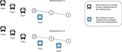
In this work, a rolling horizon can contain any number of trips within the two extreme cases. The effect of the number of considered trips in the performance of the system is investigated using real data from bus line 15L in Denver. One should note that the decision about the skipped stops of all trips within a rolling horizon is made at the start of the rolling horizon. If a rolling horizon contains a large number of trips, it is advised to re-evaluate the decisions every time a new trip is about to be dispatched to incorporate potential updates on the estimated travel times and passenger demand. This approach is commonly known as optimization in ‘rolled’ rolling horizons (Eberlein, Wilson, and Bernstein 2001) and strives to incorporate the most recent information to the decision problem. At this point, we should note that once a trip is dispatched its skipped stops cannot be modified. For instance, let us consider a rolling horizon with trips $N=⟨1,2,\dots ,|N|$. The skipped stops of those trips are decided in this rolling horizon. If a trip (e.g. trip 1) has been dispatched before the beginning of the next rolling horizon, its skipped stops cannot be modified. However, the skipped stops of trips $2,3,\dots ,|N|⟩$ that have not been dispatched yet can be modified in the next rolling horizon (see Figure 1).

Figure 1. Illustration of trips that we can modify their stop-skipping plans in two consecutive rolling horizons.

In the remainder of this section, we introduce the mathematical model of the stop-skipping problem in rolling horizons starting from the main assumptions and the nomenclature.

3.1. Assumptions and nomenclature

The modeling part of this work relies on the following assumptions:

1. Buses that serve the same line do not overtake each other. This is a common assumption in related works (see Xuan, Argote, and Daganzo 2011; Chen, Adida, and Lin 2013; Gkiotsalitis and Van Berkum 2020);

2. The passenger arrivals at stops are random because the passengers cannot coordinate their arrivals with the arrival times of buses at regularity-based services (Welding 1957; Randall et al. 2007);

3. Passengers traveling between any origin-destination pair cannot be skipped by two consecutive bus trips of the same line (Fu, Liu, and Calamai 2003; Sun and Hickman 2005; Liu et al. 2013);

4. Passengers use the same door channels for boardings and alightings.

Before proceeding to the modeling, we introduce the following nomenclature:

Nomenclature

Sets	=
N	=	ordered set of bus trips in a rolling horizon, $N=⟨1,\dots n,\dots ,|N|⟩$. Note that trip 1 is the first trip to be dispatched in this rolling horizon;
S	=	set of ordered bus stops, $S=⟨1,\dots ,s,\dots ,|S|⟩$;
Parameters	=
$\mathbf{T}$	=	is a $|N|\times (|S|-1)$ matrix of running times. Each element $t_{n,s}\in {\mathbb{R}}_{\ge 0}$ of matrix $\mathbf{T}$ is the expected running time of the nth trip between stop s−1 and s, where $s\in S\setminus \left\{1\right\}$;
$\mathbf{g}$	=	is an $|N|$-valued vector indicating the capacity of each bus trip $n\in N$;
$r_1$	=	average boarding time per passenger, a constant;
$r_2$	=	average alighting time per passenger, a constant;
δ	=	average bus acceleration plus deceleration time for serving a bus stop, a constant;
$\mathbf{\Lambda }$	=	$|S|\times |S|$ matrix where each element ${\lambda }_{sy}\in {\mathbb{R}}_{\ge 0}$ of matrix $\mathbf{\Lambda }$ denotes the average passenger arrival rate at stop s whose destination is stop y (note: ${\lambda }_{sy}=0,\mathrm{\forall }1\le y\le s$);
$c_1$	=	unit time value associated with the passenger waiting times ($/h);
$c_2$	=	unit time value associated with the passenger in-vehicle travel time ($/h);
$c_3$	=	unit time value associated with the vehicle operation time ($/h);
${\tilde{d}}_{n,1}$	=	planned departure time of every trip $n\in N$ from the first stop;
${\tilde{w}}_{1,sy}$	=	number of passengers waiting for trip 1, which is the first trip of the rolling horizon, and traveling from stop $s\in S$ to stop $y\in S$;
${\tilde{x}}_s$	=	$x_s=0$ if the already dispatched trip that precedes trip 1 when our rolling horizon starts will skip stop $s\in S$, and $x_s=1$ otherwise;
Decision variables	=
$\mathbf{x}$	=	$|N|\times |S|$-dimensional matrix of the decision variables where each $x_{n,s}\in \mathbf{x}$ can take a binary value $\{0,1\}$ with $x_{n,s}=1$ denoting that the nth bus trip will serve stop s.
Variables	=
$\mathbf{D}$	=	$|N|\times |S|$ matrix of departure times where $d_{n,s}\in {\mathbb{R}}_{{\ge }_0}$ is the departure time of trip n from stop s, where $n\in N$ and $s\in S$;
$\mathbf{A}$	=	$|N|\times |S|$ matrix of arrival times where $a_{n,s}\in {\mathbb{R}}_{{\ge }_0}$ is the arrival time of trip n at stop s, where $n\in N$ and $s\in S$;
$\mathbf{K}$	=	$|N|\times |S|$ matrix of dwell times where $k_{n,s}\in {\mathbb{R}}_{{\ge }_0}$ is the dwell time of trip n at stop s, where $n\in N$ and $s\in S$;
$\mathbf{H}$	=	$(|N|-1)\times |S|$ matrix of headways where $h_{n,s}\in {\mathbb{R}}_{\ge 0}$ is the time headway between the departure of trip n−1 and the arrival of trip n at stop s, where $n\in N\setminus \left\{1\right\}$ and $s\in S$;
$\mathbf{W}$	=	$|N|\times |S|\times |S|$ matrix where each $w_{n,sy}\in \mathbf{W}$ denotes the number of passengers waiting for bus n and traveling from stop s to y (note: $w_{n,sy}=0,\mathrm{\forall }y\le s$);
$\mathbf{L}$	=	$|N|\times |S|\times |S|$ matrix where each $l_{n,sy}\in {\mathbb{R}}_{\ge 0}$ denotes the number of passengers traveling from stop s to stop y skipped by bus n (note: $l_{n,sy}=0,\mathrm{\forall }y\le s$);
$\mathbf{M}$	=	$|N|\times |S|$ matrix where each $m_{n,s}\in {\mathbb{R}}_{\ge 0}$ denotes the number of passengers at stop s skipped by bus n, where $n\in N,s\in S$ (note: $m_{n,s}=\sum _{i=s+1}^{\mid S\mid }{l}_{n,si}$);
$\mathbf{U}$	=	$|N|\times |S|$ matrix where each $u_{n,s}\in {\mathbb{R}}_{\ge 0}$ denotes the number of passengers boarding bus n at stop s, where $n\in N,s\in S$ (note: $u_{n,\mid S\mid }=0,\mathrm{\forall }n\in N$);
$\mathbf{B}$	=	$|N|\times |S|\times |S|$ matrix where each $b_{n,sy}\in {\mathbb{R}}_{\ge 0}$ denotes the number of passengers boarding bus n at stop s whose destination is stop y (note: $b_{n,sy}=0,\mathrm{\forall }y\le s$);
$\mathbf{V}$	=	$|N|\times |S|$ matrix where each ${\nu }_{n,s}\in {\mathbb{R}}_{\ge 0}$ denotes the number of passengers alighting bus n at stop s, where $n\in N,s\in S$ (note: ${\nu }_{n,1}=0,\mathrm{\forall }n\in N$);
$\mathit{\mu }$	=	$|S|$-valued vector, where each ${\mu }_s\in {\mathbb{R}}_{\ge 0}$ denotes the average passenger arrival rate at stop s (note: ${\mu }_s=\sum _{i=s+1}^{\mid S\mid }{\lambda }_{si}$).
$\mathbf{\Gamma }$	=	$|N|\times |S|-1$ matrix where each ${\gamma }_{n,s}\in {\mathbb{R}}_{\ge 0}$ denotes the bus load of vehicle n when traveling from stop s to stop s + 1.

3.2. Variable values

Our formulation differs from the common formulations of the dynamic stop-skipping problem because it considers all trips, $N=⟨1,\dots ,n,\dots ,|N|⟩$, within a rolling horizon when determining the skipped stops.

The number of passengers destined to bus stop y who are stranded by bus trip n at stop $s,l_{n,sy}$, will be 0 if bus trip n serves stops s and y. Otherwise, it will equal the number of passengers waiting for bus trip n at stop s and have bus stop y>s as their destination. Therefore, the value of variable $l_{n,sy},\mathrm{\forall }n\in N,\mathrm{\forall }s\in S\setminus |S|,\mathrm{\forall }y\in S$ can be calculated as: (1) $l_{n,sy}\triangleq \left\{\begin{array}{ll}0,& \mathrm{i}\mathrm{f}y\le s\\ w_{n,sy}-w_{n,sy}{x}_{n,s}{x}_{n,y},& \mathrm{i}\mathrm{f}y>s\end{array}\right.$(1) Additionally, the number of passengers at stop s skipped by bus trip n is: (2) $m_{n,s}\triangleq \sum _{y=s+1}^{|S|}{l}_{n,sy},\mathrm{\forall }n\in N,s\in S\setminus \left\{|S|\right\}$(2) The number of passengers waiting for bus n at stop s whose destination is stop y>s depends on the number of passengers skipped by bus n−1 at stop s, $l_{n-1,sy}$, and the average number of passengers who arrive at stop s after bus n−1 leaves stop s: (3) $w_{n,sy}\triangleq \left\{\begin{array}{ll}{l}_{n-1,sy}+{\lambda }_{sy}{h}_{n,s},& \mathrm{\forall }n\in N\setminus \left\{1\right\},\mathrm{\forall }s\in S\setminus \left\{|S|\right\}\\ {\tilde{w}}_{1,sy},\mathrm{f}\mathrm{o}\mathrm{r}n=1,& \mathrm{\forall }s\in S\setminus \left\{|S|\right\}\end{array}\right.$(3) Note that $w_{n,sy}={\tilde{w}}_{1,sy},\mathrm{f}\mathrm{o}\mathrm{r}n=1,\mathrm{\forall }s\in S\setminus \left\{|S|\right\}$ reflects the boundary condition which is imposed at the first trip of the rolling horizon. The value of ${\tilde{w}}_{1,sy}$ does not depend on the decisions in this rolling horizon. Hence, in the current rolling horizon ${\tilde{w}}_{1,sy}$ is a parameter.

The expected number of passengers who will board bus trip n at stop s (assuming bus n stops at stop s) depends on the number of passengers traveling between stops s and $y(y>s)$ and whether the bus will stop at stop y: (4) $u_{n,s}\triangleq x_{n,s}\sum _{y=s+1}^{|S|}{w}_{n,sy}{x}_{n,y},\mathrm{\forall }n\in N,s\in S\setminus \left\{|S|\right\}$(4) Note that at the last stop we have no boardings. Thus, we introduce the boundary condition: (5) $u_{n,|S|}=0,\mathrm{\forall }n\in N$(5) From the total amount of passengers boarding bus trip n at stop s ($u_{n,s}$), the number of passengers boarding bus trip n at stop $s\in S\setminus \left\{|S|\right\}$ whose destination is stop y is: (6) $b_{n,sy}\triangleq \left\{\begin{array}{ll}{x}_{n,s}{w}_{n,sy}{x}_{n,y},& \mathrm{i}\mathrm{f}y>s\\ 0,& \mathrm{i}\mathrm{f}y\le s\end{array}\right.$(6) The expected number of alighting passengers for bus trip n at stop s depends on the number of passengers traveling between stops y and $s(y<s)$ and whether the bus will make stop y. Thus, the value of ${\nu }_{n,s}$, $\mathrm{\forall }n\in N,s\in S\setminus \left\{1\right\}$ can be derived by (7) ${\nu }_{n,s}\triangleq x_{n,s}\sum _{y=1}^{s-1}{w}_{n,ys}{x}_{n,y},\mathrm{\forall }n\in N,s\in S\setminus \left\{1\right\}$(7) A special case is the first stop of a bus trip where we do not have passenger alightings. This introduces the boundary condition: (8) ${\nu }_{n,1}=0,\mathrm{\forall }n\in N$(8) The dwell time of each bus trip n at each stop s depends on the number of passengers that will board and alight at the stop, denoted by $u_{n,s}$ and ${\nu }_{n,s}$, respectively: (9) $k_{n,s}\triangleq r_1{u}_{n,s}+r_2{\nu }_{n,s},\mathrm{\forall }n\in N,s\in S\setminus \left\{1\right\}$(9) Note that if passengers use different door channels for boardings/alightings; then, the dwell time can be expressed as $k_{n,s}\triangleq max(r_1{u}_{n,s};r_2{\nu }_{n,s})$.

The bus load of any trip $n\in N$ when it is traveling from stop s to stop s + 1 is also derived by: (10) ${\gamma }_{n,s}\triangleq \left\{\begin{array}{ll}{u}_{n,1},& \mathrm{i}\mathrm{f}s=1\\ {\gamma }_{n,s-1}+u_{n,s}-{\nu }_{n,s},& \mathrm{i}\mathrm{f}1<s<|S|\end{array}\right.$(10) When deciding about the skipped stops, it will be beneficial if the bus load of any trip n when traveling from stop s to s + 1, ${\gamma }_{n,s}$, does not exceed its capacity $g_n$. This can be achieved by adding the inequality constraint: (11) ${\gamma }_{n,s}\le g_n,\mathrm{\forall }n\in N,\mathrm{\forall }s\in S\setminus \left\{|S|\right\}$(11) The arrival time of bus trip n at stop s is equal to its departure time at stop s−1 ($d_{n,s-1}$), plus the travel time between the two stops, plus the time lost in acceleration and deceleration: (12) $a_{n,s}\triangleq d_{n,s-1}+t_{n,s}+\frac{\delta }{2}(x_{n,s-1}+x_{n,s}),\mathrm{\forall }n\in N,s\in S\setminus \{1,2\}$(12) Equation (12(12) $a_{n,s}\triangleq d_{n,s-1}+t_{n,s}+\frac{\delta }{2}(x_{n,s-1}+x_{n,s}),\mathrm{\forall }n\in N,s\in S\setminus \{1,2\}$(12) ) requires a boundary condition for the arrival time at the second stop, $a_{n,2},\mathrm{\forall }n\in N$. This is provided by the originally planned dispatching time ${\tilde{d}}_{n,1}$ of every trip $n\in N$: (13) $a_{n,2}\triangleq {\tilde{d}}_{n,1}+t_{n,2}+\frac{\delta }{2}(x_{n,1}+x_{n,2}),\mathrm{\forall }n\in N$(13) In addition, the departure time of bus trip n from stop $s\in S\setminus \left\{1\right\}$ is equal to its arrival time at that stop plus the dwell time $k_{n,s}$: (14) $d_{n,s}\triangleq a_{n,s}+k_{n,s},\mathrm{\forall }n\in N,s\in S\setminus \left\{1\right\}$(14) Assuming that overtaking between buses of the same line is not allowed, the time headway between the arrival of bus trip n at stop s and the departure of its preceding one from stop s is: (15) $h_{n,s}\triangleq a_{n,s}-d_{n-1,s},\mathrm{\forall }n\in N\setminus \left\{1\right\},s\in S\setminus \left\{1\right\}$(15) Finally, note that the time headway at the first stop is calculated based on the boundary condition that considers planned departure times of the respective trips: (16) $h_{n,1}\triangleq {\tilde{d}}_{n,1}-{\tilde{d}}_{n-1,1},\mathrm{\forall }n\in N\setminus \left\{1\right\}$(16)

3.3. Objective function

Stop-skipping strategies can have several (occasionally conflicting) objectives such as the minimization of passenger waiting times, on-board passenger delays and trip travel times. This yields a binary, multi-objective optimization problem that can be formulated with the use of weight factors $c_1,c_2,c_3$ (that convert all values to common units of cost in dollars) in order to minimize the equivalent weighted cost of passenger waiting time and passenger in-vehicle time as well as vehicle travel time: (17) $\begin{array}{rl}f\left(\mathbf{x}\right)& \triangleq c_1\sum _{n=2}^{|N|}\sum _{s=1}^{|S|-1}[(u_{n,s}-m_{n-1,s})\frac{h_{n,s}}{2}+m_{n-1,s}(\frac{h_{n-1,s}}{2}+k_{n-1,s}+h_{n,s})]\\ & +c_2\sum _{n=2}^{|N|}\sum _{s=1}^{|S|-1}\sum _{y=s+1}^{|S|}[b_{n,sy}\sum _{z=s+1}^y(t_{n,z}+(k_{n,z}+\delta \left)x_{n,z}\right)]\\ & +c_3\sum _{n=2}^{|N|}\sum _{s=2}^{|S|}(t_{n,s}+(k_{n,s}+\delta \left)x_{n,s}\right)\end{array}$(17) where the generalized cost of the objective function includes three terms. The first term includes two components. The first component, $(u_{n,s}-m_{n-1,s})\left(h_{n,s}/2\right)$, computes the total waiting time of the passengers who arrive after the departure (or passing) of bus n−1 at stop s, assuming random arrivals with an average passenger waiting time equal to half the headway. The second component represents the total waiting time of those passengers who have been stranded by bus n−1 ($m_{n-1,s}$) and have to wait for an average amount of time equal to $m_{n-1,s}(h_{n-1,s}/2+k_{n-1,s}+h_{n,s})$ because we do not allow two consecutive bus trips to skip the same origin-destination pair. The second term of the objective function calculates the total in-vehicle time of passengers summed over all O-D pairs and the final term computes the total bus trip time.

Incorporating the previously formulated vehicle movement equations, yields the following mathematical program: (18) $\begin{array}{rl}\left(Q\right):\underset{\mathbf{x}}{min}& f\left(\mathbf{x}\right)\end{array}$(18) (19) $\begin{array}{rl}\mathrm{s}.\mathrm{t}.& \mathbf{x}\in \mathcal{F}\left(x\right)=\{\mathbf{x}\mid \mathbf{x}\text{ satisfies Equations~(1){--}(16)}\}\end{array}$(19) (20) $\begin{array}{rl}& x_{n,1}=x_{n,|S|}=1,\mathrm{\forall }n\in N\end{array}$(20) (21) $\begin{array}{rl}& \left(x_{n-1,s}{x}_{n-1,y}\right)+\left(x_{n,s}{x}_{n,y}\right)\ge 1,\mathrm{\forall }n\in N\setminus \left\{1\right\},\mathrm{\forall }s\in S,\mathrm{\forall }y\ge s\end{array}$(21) (22) $\begin{array}{rl}& \left({\tilde{x}}_s{\tilde{x}}_y\right)+\left(x_{1,s}{x}_{1,y}\right)\ge 1,\mathrm{\forall }s\in S,\mathrm{\forall }y\ge s\end{array}$(22) (23) $\begin{array}{rl}& x_{n,s}\in \{0,1\},\mathrm{\forall }n\in N,\mathrm{\forall }s\in S\end{array}$(23) Note that the equality constraint of Equation (20(20) $\begin{array}{rl}& x_{n,1}=x_{n,|S|}=1,\mathrm{\forall }n\in N\end{array}$(20) ) ensures that the first and last stops of a bus trip cannot be skipped and the inequality constraints of Equations (21(21) $\begin{array}{rl}& \left(x_{n-1,s}{x}_{n-1,y}\right)+\left(x_{n,s}{x}_{n,y}\right)\ge 1,\mathrm{\forall }n\in N\setminus \left\{1\right\},\mathrm{\forall }s\in S,\mathrm{\forall }y\ge s\end{array}$(21) ) and (22(22) $\begin{array}{rl}& \left({\tilde{x}}_s{\tilde{x}}_y\right)+\left(x_{1,s}{x}_{1,y}\right)\ge 1,\mathrm{\forall }s\in S,\mathrm{\forall }y\ge s\end{array}$(22) ) that if an origin-destination pair is skipped by one trip, it will be served by the next one.

Program $\left(Q\right)$ is an integer nonlinear programming problem (INLP) and it is solved every time a new rolling horizon starts. Due to its combinatorial nature, the problem can be solved to global optimality with an exhaustive search of the solution space. Exploring the entire solution space with brute force results in exponential computational complexity. This is formally proved in Theorem 3.1.

Theorem 3.1

The rolling horizon stop-skipping problem, $\left(Q\right),$ is at least an NP-complete decision problem with an exponential computational complexity that requires to explore $2^{|N|\times |S|}$ potential solutions to obtain a globally optimal one.

Proof.

Given that the constraints limit $x_{n,s}$ to either 0 or 1, any feasible solution to the integer program $\left(Q\right)$ is a subset of vertices. The first constraint implies that at least one end point of every edge is included in this subset. Therefore, the solution describes a vertex cover. Additionally, given some vertex cover C, $x_{n,s}$ can be set to 1 for any $(n,s)\in C$ and to 0 for any $(n,s)\notin C$, thus giving us a feasible solution to the integer program. Hence, our problem can be reduced to the minimum vertex cover which is one of Karp's 21 NP-Complete decision problems (Karp 1972) that demonstrates the NP-Hardness of problem $\left(Q\right)$. That is, there is no polynomial algorithm that can solve all instances of $\left(Q\right)$, unless P≡NP.

Now, if we want to find the globally optimal stop-skipping strategy of one trip, we need to explore a set of $2^{|S|}$ potential solutions because at each stop $s\in \{1,2,\dots ,|S|\}$ we have two options: serve or skip. In a rolling horizon with N trips, we should make a total number of $|N|\times |S|$ simultaneous stop-skipping decisions. That is, the potential solutions that need to be evaluated are $2^{|N|\times |S|}$.

Evaluating the feasibility and the performance of $2^{|N|\times |S|}$ potential stop-skipping solutions using the equations of program $\left(Q\right)$ is not a trivial task. First, an increase in the number of trips and/or stops increases exponentially the solution space. Second, and equally important, the equations of program $\left(Q\right)$ include several recursive relationships that increase the computational cost when the number of trips and stops is increased.

4. Solution methods

In this section, we present the solution methods that we will investigate for the solution of the stop-skipping problem in rolling horizons expressed in $\left(Q\right)$. An obvious solution method that returns a globally optimal solution of this discrete optimization problem is the brute force method which is described first.

Given that the brute force and B&B might not be able to scale in real-sized scenarios, we also explore other solution methods from the area of evolutionary optimization: namely, the sequential hill climbing (S-HC) and the genetic algorithm (GA). Both methods are metaheuristics that search for a globally optimal solution. Their main advantage is the efficient exploration of the solution space without evaluating every solution option. This reduces the computational costs which (hopefully) allow attaining an improved solution in near real-time. However, evolutionary optimization methods cannot guarantee the convergence to a globally optimal solution and result in trade-offs between computational speed and solution quality.

4.1. Brute force

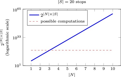
The brute force solution method evaluates exhaustively the values of the variables and the objective function covering each potential solution. To cover the entire solution space, the number of solution evaluations is $2^{|N|\times |S|}$. For a typical bus line with 20 stops, the total number of solution evaluations varies with respect to the number of trips, $|N|$. This is depicted in Figure 2 which is plotted in logarithmic scale. Figure 2 indicates that we cannot evaluate all possible solutions in near real-time for more than $|N|=3$ trips in the rolling horizon since the world's fastest supercomputer can execute up to 33,860 trillion calculations per second.

Figure 2. Required solution evaluations for a bus line with $|S|=20$ bus stops when the number of trips in the rolling horizon, $|N|$, varies. The possible computations are the computations that can be executed by the world's fastest supercomputer in 1 min.

4.2. Sequential hill climbing

In the sequential hill climbing search, the stop-skipping decision variables are initialized as $x_{n,s}=1,\mathrm{\forall }n\in N,\mathrm{\forall }s\in S$. Hence, the initial solution $\mathbf{x}$ indicates that all trips in the rolling horizon serve the entirety of stops.

The performance of this solution is evaluated by calculating the value of $f\left(\mathbf{x}\right)$ in program $\left(Q\right)$. Hill climbing attempts to minimize the objective function $f\left(\mathbf{x}\right)$ by adjusting a single element of $\mathbf{x}$ at each step and determining whether that change improves $f\left(\mathbf{x}\right)$. The S-HC search comprises of the following steps:

1. for the initial trip in the rolling horizon, n = 1;

2. for the second bus stop, s = 2;

3. change the stop-skipping status of $x_{n,s}$ by selecting a value from the set {0,1}. If the selected value reduces the value of $f\left(\mathbf{x}\right)$ and meets the constraints, this value is adopted. Otherwise, it is discarded;

4. the previous procedure is performed for all other stops $i\in S\setminus \{3,|S|-1\}$ in a sequential order;

5. the previous procedure is performed for all other trips $j\in N\setminus \left\{1\right\}$ in a sequential order;

6. the above-described procedure in steps 1–5 is repeated until reaching the maximum number of allowed iterations, ${\mu }^{max}$.

The above procedure is formalized in Algorithm 1 which is publicly released in Gkiotsalitis (2019a).

The S-HC algorithm terminates after ${\mu }^{max}$ iterations. The number of iterations is an externally defined, hyperparameter of the metaheuristic. At each main iteration, the S-HC starts from trip n = 1 and stop s = 2 and searches for stop-skipping decisions that do not violate the constraints (lines 11–13 in Algorithm 1) and improve the objective function (lines 14-16 in Algorithm 1). The term ‘sequential’ is used because stop-skipping options are evaluated in a sequential order for every trip $n\in N$ and stop $s\in S\setminus \{1,|S|\}$. That is, we do not try to improve the objective function score by changing all values of $\mathbf{x}$ at a single step.

At each iteration, the sequential hill climbing search is repeated. This allows the algorithm to avoid local minima by starting its search from another incumbent solution. This multi-start search improves the convergence of hill climbing because it spends resources on exploring the solution space, rather than carefully optimizing the initial solution (Deb 2001). Such restart is broadly used in past literature and is generally known as Shotgun hill climbing (Simon 2013). The number of objective function evaluations when using Algorithm 1 is analyzed in Theorem 4.1 and is proved to be polynomial with regards to the number of trips in the rolling horizon, $|N|$.

Theorem 4.1

The computational complexity of the S-HC metaheuristic is polynomial with a number of solution evaluations of $2|N|(|S|-2){\mu }^{max}$.

Proof.

In the algorithmic description of S-HC, the steps 8–16 that evaluate whether a change on a single stop-skipping decision is beneficial and does not violate the constraints of program $\left(Q\right)$ require one evaluation of the objective function score. At each main iteration (1,2,…,${\mu }^{max}$), steps 8-16 are performed $2|N|(|S|-2)$ times. Consequently, the total number of objective function evaluations is $2|N|(|S|-2){\mu }^{max}$ and depends on the hyperparameter ${\mu }^{max}$. Note that if we set ${\mu }^{max}=1$, the required objective function evaluations are fixed: $2|N|(|S|-2)$.

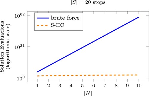
To compare the number of solution evaluations of the S-HC algorithm and the brute force method, we plot in Figure 3 the required solution evaluations of both algorithms for rolling horizons with 1–10 trips, a bus line with 20 stops, and ${\mu }^{max}=5$. Note that the number of computations of the S-HC increases linearly with the number of trips, $|N|$, in the rolling horizon. This linear increase is depicted in Figure 3 in the form of a horizontal line because of the logarithmic scale. Similarly, the exponential increase of the required number of solution evaluations with the use of brute force is depicted as an affine function of $|N|$.

Figure 3. Required number of objective function evaluations with brute force and S-HC for rolling horizons with 1–10 trips, a bus line with 20 stops, and ${\mu }^{max}=5$.

We should note here that even if the solution evaluations of the S-HC method increase polynomially with the number of trips and stops, this does not guarantee that we can compute a solution in large scale scenarios. The reason behind this is that the computational cost of each solution evaluation increases with the number of trips and stops because of the recursive relationships in program $\left(Q\right)$.

4.3. Genetic algorithm

In the genetic algorithm, each population member (individual) represents a potential solution of program $\left(Q\right)$. The number of population members is a hyperparameter of the GA and is externally defined. Proceeding to the encoding stage, if we have a set of population members $\mathrm{\Pi }=\{1,2,\dots ,|\mathrm{\Pi }|\}$, then each population member $\pi \in \mathrm{\Pi }$ is a $|N|\times |S|$-dimensional matrix ${\mathbf{x}}^{\pi }$ with elements ${\mathbf{x}}_{n,s}^{\pi }\in \{0,1\},\mathrm{\forall }n\in N,\mathrm{\forall }s\in S$. In the GA terminology, each element ${\mathbf{x}}_{n,s}^{\pi }$ is known as a gene of the individual ${\mathbf{x}}^{\pi }$. Using this terminology, the GA comprises of the following steps:

1. Encoding: initially, the individuals of the population $\mathrm{\Pi }=\{1,2,\dots ,|\mathrm{\Pi }|\}$ can be generated randomly by selecting a random value from the 0-1 set for each ${\mathbf{x}}_{n,s}^{\pi },\mathrm{\forall }n\in N,\mathrm{\forall }s\in S\setminus \{1,|S|\},\mathrm{\forall }\pi \in \mathrm{\Pi }$. Note that the trips cannot skip their first and last stop, hence ${\mathbf{x}}_{n,1}^{\pi }=1$ and ${\mathbf{x}}_{n,|S|}^{\pi }=1,\mathrm{\forall }n\in N,\mathrm{\forall }\pi \in \mathrm{\Pi }$. In addition, we initialize the counter of iterations, $\mu =1$.

2. Selection of the fittest: from the population, the fittest parents should be selected for reproduction. This is achieved by using the well-known roulette-wheel selection method (Goldberg and Deb 1991). In the roulette-wheel selection method, each individual π has a probability of being selected which is proportional to its fitness value. Note that GAs seek to maximize fitness. In contrast, the stop-skipping problem in rolling horizons seeks to minimize the score of our objective function $f\left(\mathbf{x}\right)$ in program $\left(Q\right)$. Hence, one population member $\pi \in \mathrm{\Pi }$ is more fit if the value of $-f\left({\mathbf{x}}^{\pi }\right)$ is higher (that is, it maximizes fitness). Note also that population members that violate the constraints of program $\left(Q\right)$ are not selected as parents. The parent selection process terminates when the number of selected parents is the same as the population size $|\mathrm{\Pi }|$ to ensure that the generated offsprings will maintain our population size.

3. Crossover: pairs of parents generate new population members (offsprings) at the crossover stage. Two parents exchange their genes at a randomly selected crossover point for generating two offsprings. For instance, if the crossover point of two parents π and $\hat{\pi }$ is n, s; then, the two generated offsprings will have the set of genes $({\mathbf{x}}_{1,1}^{\pi },\dots ,{\mathbf{x}}_{n,s}^{\pi },{\mathbf{x}}_{n,s+1}^{\hat{\pi }},\dots ,{\mathbf{x}}_{|N|,|S|}^{\hat{\pi }})$ and $({\mathbf{x}}_{1,1}^{\hat{\pi }},\dots ,{\mathbf{x}}_{n,s}^{\hat{\pi }},{\mathbf{x}}_{n,s+1}^{\pi },\dots ,{\mathbf{x}}_{|N|,|S|}^{\pi })$ respectively. If the generated offspring is infeasible, the crossover is repeated selecting another crossover point.

4. Mutation: each generated offspring is subject to mutation. The mutation helps the GA to explore new areas of the solution space and avoid getting trapped in local minima. In our case, we specify a small probability, $p_c$, for replacing each gene of the generated offspring with a random value from the set $\{0,1\}$. The mutation is allowed only if the offspring remains feasible. Note that this probability is set to zero if the stop-skipping decision refers to stops 1 or $|S|$ because a trip cannot skip its first or last stop.

5. Termination: with the crossover and mutation stages, the population members evolve and create a new population generation where the offsprings replace their parents. Then, we continue by setting $\mu \leftarrow \mu +1$ and repeating steps (2)-(4). The procedure described above continues iteratively until a pre-determined number of population generations, ${\mu }^{max}$, is reached. That is, $\mu ={\mu }^{max}$. The population member with the best performance is then selected as the stop-skipping solution.

The above algorithm has three hyperparameters which must be externally defined prior to its implementation: (a) the population size $|\mathrm{\Pi }|$, (b) the mutation rate $p_c$, and (c) the maximum number of population generations ${\mu }^{max}$. Two of those hyperparameters, namely $|\mathrm{\Pi }|$ and ${\mu }^{max}$, affect the computational cost of the GA because they increase directly the number of evaluations of the objective function. In more detail, at each population generation, the objective function should be evaluated $|\mathrm{\Pi }|$ times to determine the fitness of each population member. For a total of ${\mu }^{max}$ population generations, the required evaluations of the objective function would rise to $|\mathrm{\Pi }|{\mu }^{max}$.

One should note that the hyperparameters of the metaheuristics must be determined on a trial-and-error basis considering the efficiency of the optimization algorithm. For instance, reducing the population size of a GA will reduce its computational costs, but, at the same time, it will limit the solution space exploration and (most probably) the quality of the solution if all other hyperparameter values remain the same. Given that we need a solution method that can perform in near real-time, the hyperparameter values should be adjusted accordingly.

5. Numerical experiments

5.1. Computational tests and solution quality in a toy network

In this subsection, we perform computational tests of the three solution methods in a toy network of idealized scenarios. The aim is twofold: (i) to investigate the computational times of the algorithms and (ii) to evaluate the optimality gap of the metaheuristics (S-HC and GA). To determine the optimality gap of a solution method, we need to compute a globally optimal solution with the use of brute force. However, a globally optimal solution can be computed only in small-scale instances where the stop-skipping candidates are limited. Therefore, the optimality gap of the metaheuristics is examined in rolling horizons with a limited number of trips and stops.

The computational tests are performed in a general-purpose computer with Intel Core i7-455 7700HQ CPU @ 2.80GHz and 16 GB RAM. To facilitate the reproduction of our results, we provide below the input data of our computational tests in the toy network.

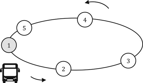
In the toy network, we consider a circular bus line with 5 bus stops, as presented in Figure 4. We also consider up to 4 trips in the rolling horizon, and fixed travel times $t_{n,s}=60\mathrm{s}$, $\mathrm{\forall }n\in N,\mathrm{\forall }s\in S\setminus \left\{1\right\}$. Additionally, the average number of passenger arrival rate at stop $s\in S$ whose destination is stop $y\in S$ is set to ${\lambda }_{n,sy}=1$ passenger per minute if y>s and 0 if $y\le s$. The number of passengers waiting for trip 1, which is the first in this rolling horizon, and traveling from stop $s\in S$ to stop $y\in S$ is set as ${\tilde{w}}_{1,sy}=12$ if y>s and 0 otherwise. In addition, the capacity of each vehicle $n\in N$ is $g_n=75$ passengers and the previous trip that precedes the first trip in our rolling horizon does not skip any stops (${\tilde{x}}_s=1,\mathrm{\forall }s\in S$).

Figure 4. Topology of the toy network operating one bus line.

The values of the other parameters of the idealized scenario(s) in this toy network are presented in Table 1.

Table 1. Parameter values of the idealized scenario.

Parameter	Value	Parameter	Value
$r_1$	2 s	$c_1$	10 $/h
$r_2$	1 s	$c_2$	5 $/h
δ	20 s	$c_3$	7 $/h

Finally, the planned dispatching times of the 4 trips are ${\tilde{d}}_{n,1}=600(n-1),\mathrm{\forall }n\in \{1,2,\dots ,4\}$. That is, trip n = 1 is dispatched at ${\tilde{d}}_{n,1}=0$ s, trip n = 2 at ${\tilde{d}}_{n,1}=600$ s and so forth. This indicates a 10-min dispatching headway among trips.

To demonstrate the application of our model, we first evaluate the cost of the objective function of program $\left(Q\right)$ for any potential stop-skipping combination when we have $|N|=4$ trips in the rolling horizon. This requires $s^{|N|\times |S|}=2^{20}$ evaluations of the objective function with the brute force method. The mathematical program $\left(Q\right)$ is programmed in Haskell 8.6.3. The source code is publicly released at Gkiotsalitis (2019a) to facilitate the reproduction of our model.

The globally optimal solution in this rolling horizon when evaluating all possible stop-skipping options with brute force is: ${\mathbf{x}}^{\ast }=\left[\begin{array}{ccccc}1& 1& 1& 1& 1\\ 1& 1& 1& 1& 1\\ 1& 1& 1& 1& 1\\ 1& 0& 0& 0& 1\end{array}\right]$ with a generalized objective function cost, $f\left({\mathbf{x}}^{\ast }\right)=563,491\mathrm{\$}$ The computational cost of evaluating all possible stop-skipping options with brute force for the case of 5 stops and 4 trips is 353 s. Due to the exponential increase of the computational cost when using the brute force method, a globally optimal solution cannot be computed when we consider more than 5 stops. This is reported in Table 2 that summarizes the computational times of brute force, S-HC, and GA in our idealized bus line considering an increasing number of stops. We also report the results of solving program $\left(Q\right)$ with an off-the-shelf optimization solver (LINDO 10.0) that cannot always guarantee global optimality due to the nature of our problem. Note that the hyperparameters of the genetic algorithm (namely, the population size, the mutation rate, and the maximum population generations) have been calibrated for each scenario to guarantee that it will attain its best performance when compared against the other solution methods. Their values are 52 population members, 4 population generations, and a mutation rate of 0.4.

Table 2. Computational costs and optimality gap(s) when applying Brute Force (BF), S-HC and the GA in the idealized bus line for different numbers of stops.

	Comput. Time (s)				Optimized $f\left(\mathbf{x}\right)$ ($)
Stops	BF	LINDO	S-HC	GA	BF	LINDO	S-HC	GA
3	0.11	0.19	0.96	1.03	169,101	169, 101	169,101	169,101
4	15.88	6.70	4.32	5.12	326,688	326,688	326,688	326,688
5	353.12	98.21	7.68	17.21	563,491	563, 491	563,491	595,819
6	−	259.19	21.62	41.89	−	897, 533	897,533	982,738

From Table 2 one can note that the solution of the brute force method and the solutions of the S-HC and GA are identical in the cases of 3 or 4 bus stops. In the case of 5 stops, the optimality gap of the GA is 5.4%. For more than 5 bus stops, the optimality gap cannot be established because the brute force method cannot compute a globally optimal solution resulting in the absence of a benchmark.

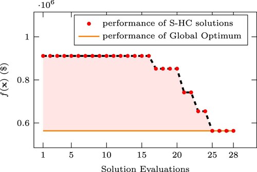
In general, the S-HC algorithm converged faster than the GA and required fewer solution evaluations until its termination. This is reflected in its computational time which is significantly lower than the GA one. To provide a tangible example of the required solution evaluations with different solution methods, we report the solution evaluations when using the S-HC method in the case of 5 stops and 4 trips in Figure 5. From Figure 5, one can note that the S-HC method required only 28 solution evaluations until convergence, whereas the brute force method had to explore the entire solution space, and thus perform $2^{20}=1,048,576$ evaluations to solve the same problem.

Figure 5. Convergence of the S-HC algorithm in the case of 5 bus stops and 4 trips in the rolling horizon.

Although the required solution evaluations with S-HC or GA are very limited compared to the brute force method, the computational times of S-HC and GA increase significantly with the number of stops. Given that the required solution evaluations increase linearly with the number of stops and trips, this indicates that the computational cost of evaluating the performance of each solution exhibits a disproportionate increase with the number of stops.

This can be explained because of the recursive relationships in program $\left(Q\right)$. As expected, the recursive relationships result in increased computational costs for evaluating the performance of one solution when the number of stops increases. To further investigate this, detailed computational times for the evaluation of one solution with respect to the number of stops are presented in Figure 6.

Figure 6. Computational cost when evaluating the performance of a single solution in a rolling horizon with 4 bus trips with respect to the number of stops.

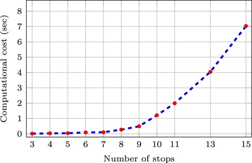
Evidently, the sole reason for the increase in computational costs when using metaheuristics is the increasing costs for evaluating the performance of a solution in more complex scenarios. Indeed, for 11 candidate stops we require almost 2 s to evaluate the performance of a single solution (cf. Figure 6). Applying the S-HC method with ${\mu }^{max}=6$ requires the exploration of 2$|N|(|S|-2){\mu }^{max}=2\cdot 4\cdot 9\cdot 6=432$ solution candidates, or around $432\cdot 2=864$ s. Consequently, even with the use of metaheuristics, the stop-skipping candidate stops need to be carefully selected to limit their total number.

5.2. Sensitivity analysis with respect to travel time variations

In the previous subsection, we performed the computational cost and optimality gap analysis of the three proposed solution methods demonstrating the need for limiting the stop-skipping candidate stops. Herein, we investigate the sensitivity of the optimal solution to travel time variations during the actual operations. To perform this task, the following numerical examples are abstracted using real data from bus line 15L in Denver, US.

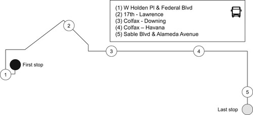
Bus line 15L (cf. Figure 7) is a bus line with 42 bus stops that connects the eastern part of the Denver metropolitan area with a train station at the southwest (Aurora Metro Center). Bus line 15L serves the downtown area of the city. The first trip of the day is planned at 6:02 am and the last trip of the day is expected to arrive at the terminal at 1:03 am. From the 42 stops, we select 5 stops as stop-skipping candidates in order to be able to compute a stop-skipping solution in near real-time. All stops, except stop 2, are in areas with low passenger demand to fully exploit the potential benefit of skipped stops. The timetable information is publicly available at Regional Transportation District (2019) and the stops under consideration are presented in Figure 7.

Figure 7. Stop-skipping candidates of bus line 15L in Denver.

All stops in Figure 7 can be skipped by the bus trips in the rolling horizon. Considering data from the real operations, the original headway on a typical Saturday is 18 minutes resulting in 61 daily trips. As in Fu, Liu, and Calamai (2003), the passenger boarding and alighting times are assumed to be 4 and 2 s per passenger, respectively. In addition, in accordance with Fu, Liu, and Calamai (2003), values of $20/h, $10/h, and $50/h are used for the objective function weighting factors $c_1$, $c_2,$ and $c_3$, respectively. To model the effect of the bus travel time variation, we assume a normal distribution with a coefficient of variation (CV) of 0.20, 0.30, 0.40 and 0.50 for all links along the route. For every CV, we generate different simulation scenarios that allow us to investigate the performance of our stop-skipping solution to scenarios with different levels of travel time variation.

First, we compute the optimal stop-skipping solution using the expected (average) link travel time values, $\mathbb{E}\left[t_s\right]$. Those values are presented in Table 3.

Table 3. Expected travel times, $\mathbb{E}\left[t_s\right]$.

origin$\to$destination	Travel time	origin$\to$destination	Travel time
1$\to$2	660 s	3$\to$4	1200 s
2$\to$3	660 s	4$\to$5	1080 s

Other parameter values considered in the computation of the optimal stop-skipping solution for the nominal (average) case are: δ=20 s, ${\tilde{w}}_{1,sy}=12$ passenger if y>s and ${\tilde{w}}_{1,sy}=0$ otherwise. The vehicle capacity is 80 passengers. According to the timetable of bus line 15L, the dispatching times of the first 4 trips of the day are 6:02 am, 6:32 am, 7:02 am, and 7:26 am, respectively. This yields expected headways of 30, 30, 30, and 24 min, respectively. We hereby note that even if the headways of our four selected trips are relatively long, our bus line is a high-frequency bus line and operates under a regularity-based scheme. That is, passengers are not fully informed about the expected time of arrival of every bus trip and this increases the chances that they will not be able to fully coordinate their arrival times at stops with the arrival times of buses.

Based on this abstracted scenario that uses the available real data from bus line 15L, the optimal stop-skipping solution of the first 4 trips of the day is: ${\mathbf{x}}^{\ast }=\left[\begin{array}{ccccc}1& 1& 1& 1& 1\\ 1& 0& 1& 1& 1\\ 1& 1& 1& 1& 1\\ 1& 1& 0& 0& 1\end{array}\right]$ with a generalized objective function cost, $f\left({\mathbf{x}}^{\ast }\right)=85,192,498\mathrm{\$}$ To investigate the sensitivity of the nominal solution, we perform a simulation-based evaluation of its performance for different travel time variation levels. To reduce the sampling bias in our simulation, we perform a large number of 1000 Monte Carlo simulations for each CV level (0.20, 0.30, 0.40, and 0.50). In each Monte Carlo simulation, we consider a rolling horizon with $n=⟨1,2,3,4⟩$ trips (the first 4 trips of the day) and we sample their link travel times from the normal distribution with mean $\mathbb{E}\left[t_s\right]$ and standard deviation $\mathrm{C}\mathrm{V}\cdot \mathbb{E}\left[t_s\right]$. That is, ${\tilde{t}}_{n,s}^j\sim \mathcal{N}\left(\mathbb{E}\right[t_s],\mathrm{C}\mathrm{V}\cdot \mathbb{E}[t_s\left]\right)$ where j is the respective simulation scenario.

In extreme cases, sampling link travel times ${\tilde{t}}_{n,s}^j$ from a normal distribution might yield unreasonable values (i.e. negative travel times). To rectify this, we use a lower bound, $t_s^{min}$, which is the minimum possible travel time from stop s to stop s + 1 under free-flow conditions, and an upper bound, $t_s^{max}$, which is the maximum possible travel time observed in congestion peaks. Those bounds yield realistic simulation scenarios with sampled travel times, $t_{n,s}^j$, as follows: (24) $t_{n,s}^j=\{t_s^{min},{\tilde{t}}_{n,s}^j,t_s^{min}\},\mathrm{\forall }n\in N,\mathrm{\forall }s\in S$(24) where j indicates each simulation scenario $j\in \{1,2,\dots ,1000\}$ for a given CV value.

The performance of our stop-skipping solution when applied in (i) 1000 scenarios with $\mathrm{C}\mathrm{V}=0.20$, (ii) 1000 scenarios with $\mathrm{C}\mathrm{V}=0.30$, (iii) 1000 scenarios with $\mathrm{C}\mathrm{V}=0.40$, and (iv) 1000 scenarios with $\mathrm{C}\mathrm{V}=0.50$ is presented in Figure 8 following the Tukey boxplot convention (McGill, Tukey, and Larsen 1978). The upper and lower boundaries of the boxes indicate the upper and lower quartiles (i.e. 75th and 25th percentiles denoted as Q3 and Q1, respectively). The black lines vertical to the boxes (whiskers) show the maximum and minimum values that are not outliers. The whiskers are determined by plotting the lowest datum still within 1.5 the interquartile range (IQR) Q3–Q1 of the lower quartile, and the highest datum still within 1.5 IQR of the upper quartile (McGill, Tukey, and Larsen 1978).

Figure 8. Performance when applying the optimal stop-skipping solution in 1000 simulations considering $\mathrm{C}\mathrm{V}=0.2$, 0.3, 0.4, and 0.5, respectively.

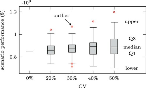
The numerical values of the median, the 25th and 75th percentiles, and the whiskers are also reported in Table 4. The median value of the performance of the generalized cost function for $\mathrm{C}\mathrm{V}=20\mathrm{\%}$ is almost equal to the theoretical performance under no travel time variation $(\mathrm{C}\mathrm{V}=0\mathrm{\%})$. In contrary, a significant deterioration occurs for $\mathrm{C}\mathrm{V}=30\mathrm{\%}$ (from 85,845$\times {10}^3$ to 90,768$\times {10}^3$, that is $6\mathrm{\%}$). The main findings are summarized below:

• for travel time variation with $\mathrm{C}\mathrm{V}=20\mathrm{\%}$, the median performance does not deteriorate significantly from the nominal (ideal) case of no travel time variation;

• for $\mathrm{C}\mathrm{V}>20\mathrm{\%}$, there is significant deterioration to the medial performance which is at the level of $6\mathrm{\%}$;

• in worst-case scenarios (outliers), the generalized cost of the objective function can increase by 40% compared to the one in the ideal case of no variation;

• for CV of more than 30%, there is an increase at the interquartile range – and not at the median;

• for $\mathrm{C}\mathrm{V}=20\mathrm{\%}$, the generalized cost of the objective function is expected to deteriorate by less than $5\mathrm{\%}$ in 75% of the cases based on the value of Q3.

Table 4. Performance when running 1000 simulations for different travel time variation levels (in thousands).

CV	Minimum	Q1	Median	Q3	Maximum
0%	85,192	85,192	85,192	85,192	85,192
20%	73,947	82,426	85,845	89,908	100,917
30%	74,503	84,123	90,768	87,759	100,637
40%	71,864	82,373	89,220	92,630	106,184
50%	70,239	82,750	88,920	95,889	110,728

To summarize, our stop-skipping solution is sensitive to travel time variations. The simulation-based analysis shows that for mild variations with $\mathrm{C}\mathrm{V}<20\mathrm{\%}$, the performance of our generalized objective function will deteriorate by at most 5% in 75% of the cases. After this level, we notice an increase in both the median and the interquartile range indicating that there can be several cases where the actual performance exhibits a significant deterioration compared to the ideal scenario.

5.3. Sensitivity analysis with respect to the number of trips at each rolling horizon

Another main parameter of our proposed method is the number of trips within a rolling horizon. In the extreme case where one rolling horizon contains only one trip, our problem is reduced to the one presented in Fu, Liu, and Calamai (2003). In another extreme case, if the trips $|N|$ are equivalent to the entire number of trips in the daily schedule, then we are solving a scheduling problem where one has to plan a stop-skipping strategy for the entire day.

In the first case, the stop-skipping solution is myopic because it computes the optimal choice for a running trip without considering its adverse effects on subsequent trips. In the latter case, the stop-skipping problem is transformed into a tactical planning problem that cannot be solved in a reasonable amount of time because of the significant increase in the decision variables.

Evidently, it is important to investigate the optimal number of trips that should be included in a rolling horizon to mitigate the negative effects associated with extreme cases. Thus, we perform a sensitivity analysis to explore the effect of the number of trips considered on a rolling horizon. From bus line 15L in Denver, we consider the first 12 trips of the day. Then, we optimize the stop-skipping options in rolling horizons that contain a different number of trips. Namely, we have 6 different scenarios:

1. 12 rolling horizons that contain 1 trip (solved by the model of Fu, Liu, and Calamai 2003);

2. 6 rolling horizons that contain 2 trips;

3. 4 rolling horizons that contain 3 trips;

4. 3 rolling horizons that contain 4 trips;

5. 2 rolling horizons that contain 6 trips;

6. 1 rolling horizon that contains all trips.

The results are reported in Figure 9 where the generalized cost of the objective function is reported for different numbers of trips in the rolling horizon. To reduce the bias in the comparative analysis, we assume that there is no travel time variation and all other conditions remain the same in all cases.

Figure 9. Performance of the stop-skipping strategy depending on the considered number of trips in a rolling horizon.

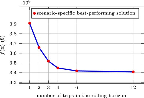
As expected, the myopic stop-skipping solution that optimizes the stop-skipping strategy of one bus trip at a time exhibits the worst performance which has an increased cost of 12.8% compared to the case where all trips are optimized simultaneously.

Interestingly, the solution quality does not improve significantly when we consider more than 4 trips in the rolling horizon. For instance, if we consider all 12 trips, the performance of the solution is only improved by a meager 1.2%. This interesting finding can be instrumental in the application of stop-skipping control at the operational level because considering rolling horizons with 4 to 6 trips mitigates the excessive computation time issues related to larger problem instances.

6. Discussion

Implementing stop-skipping strategies in rolling horizons has a significant advantage compared to the dynamic stop-skipping of a single bus trip. Notwithstanding this, exogenous factors – such as the travel time variation – can limit the potential benefit of applying a stop-skipping solution (i.e. we observed a performance deterioration of up to 40% in scenarios with $\mathrm{C}\mathrm{V}=40\mathrm{\%}$). This is in line with the reported findings from past works in timetabling (Gkiotsalitis, Eikenbroek, and Cats 2019) and bus holding (Eberlein et al. 1998).

The solution sensitivity to travel time variations underlines the need for accurate travel time predictions for trips that will be dispatched in the near future. This reinforces the need for rolling horizons with a small number of trips to avoid long-term travel time predictions that will probably be less accurate. For instance, if a rolling horizon considers all daily trips, it is very probable that the estimated travel times of trips that will occur later in the day will deviate significantly from the realized ones. In contrast, if a rolling horizon considers a small number of trips the prediction error can be much smaller. This was also discussed in the bus holding work of Eberlein et al. (1998) that suggested short rolling horizons to benefit from the accuracy of short-term travel time predictions.

The use of short rolling horizons is also reinforced from our sensitivity analysis which indicated that rolling horizons with 4 trips provide a significant benefit compared to the myopic case of considering one trip at a time and are close to solutions that consider the entirety of available trips. Especially for the stop-skipping problem, this is of paramount importance because stop-skipping is proved to be an NP-Hard, 0–1 problem which is intractable in problem instances with a large number of decision variables.

6.1. Limitations

To facilitate the reproducibility of our work, we explicitly state the main limitations that are associated with our model and the solution method(s):

• our work can be applied only in services where the passengers do not coordinate their arrivals at stops with the arrival times of the buses;

• our work cannot be applied in bus line services with a significant number of overtakes among buses that operate in the same line;

• the stop-skipping strategy in our work yields potential gains in operations with mild disruptions in terms of travel time variability. In the case of severe disruptions, other measures – such as a re-allocation of resources at the tactical planning stage – should be considered;

• our model cannot be solved to global optimality if the number of candidate stops for stop-skipping is high. Hence, a meticulous pre-selection of stop-skipping candidates is required. Note that such pre-selection can have positive secondary effects because skipping too many stops can increase the inconvenience of passengers and affect the coordination of the bus operations at the network-level.

7. Conclusion

This work investigated the stop-skipping problem in rolling horizons. It provided a problem formulation and proved the NP-completeness of this 0–1 problem. Potential solution methods, such as brute force, sequential hill climbing and a genetic algorithm, have been tested indicating that the problem can be solved for a limited number of stop-skipping candidates in quasi-real-time conditions.

The potential benefits of devising stop-skipping strategies in rolling horizons are significant in scenarios with mild disruptions (travel time variations with $\mathrm{C}\mathrm{V}<20\mathrm{\%}$). Hence, we propose to apply stop-skipping strategies in short-term rolling horizons where the accuracy of the estimated trip travel times is typically higher. That is to say, a stop-skipping strategy should consider a small fraction of imminent trips instead of the entirety of trips in the daily schedule. This argument is also reinforced by the computational complexity of the problem that does not allow to compute the skipped stops of several trips within a reasonable time.

Considering a number of trips in the range of 4–6 in each rolling horizon has a distinct benefit compared to the myopic methods of optimizing one trip at a time (i.e. Fu, Liu, and Calamai 2003) with performance improvements up to 13%. Notwithstanding the potential benefits, this research suggests some important managerial implications. One managerial implication is the proper communication of the skipped stops to passengers, bus drivers, and other stakeholders.

Other managerial implications are the pre-selection of suitable stops as stop-skipping candidates and the improvement of the accuracy of the estimated trip travel times to achieve the maximum benefit. For the former case, specific attention should be given to the network structure and potential transfer points among different bus lines to avoid missed connections because of skipped stops.

In future research, the proposed stop-skipping approach can be applied to other problems that consider the synchronization of services and the passenger transfers. Moreover, the secondary effects of a stop-skipping strategy to the implementation of the timetable and passenger satisfaction should be thoroughly studied.

Disclosure statement

No potential conflict of interest was reported by the author(s).

References

- Altazin, Estelle, Stéphane Dauzère-Pérès, François Ramond, and Sabine Tréfond. 2017. “Rescheduling Through Stop-Skipping in Dense Railway Systems.” Transportation Research Part C: Emerging Technologies 79: 73–84. doi: https://doi.org/10.1016/j.trc.2017.03.012
- Bartholdi III, John J., and Donald D. Eisenstein. 2012. “A Self-Coördinating Bus Route to Resist Bus Bunching.” Transportation Research Part B: Methodological 46 (4): 481–491. doi: https://doi.org/10.1016/j.trb.2011.11.001
- Bostel, Nathalie, Pierre Dejax, Pierre Guez, and Fabien Tricoire. 2008. “Multiperiod Planning and Routing on a Rolling Horizon for Field Force Optimization Logistics.” In The Vehicle Routing Problem: Latest Advances and New Challenges, 503–525. Springer.
- Cao, Zhichao, and Avishai Avi Ceder. 2019. “Autonomous Shuttle Bus Service Timetabling and Vehicle Scheduling Using Skip-Stop Tactic.” Transportation Research Part C: Emerging Technologies 102: 370–395. doi: https://doi.org/10.1016/j.trc.2019.03.018
- Cao, Zhichao, Zhenzhou Yuan, and Silin Zhang. 2016. “Performance Analysis of Stop-Skipping Scheduling Plans in Rail Transit Under Time-Dependent Demand.” International Journal of Environmental Research and Public Health 13: 707. doi: https://doi.org/10.3390/ijerph13070707
- Ceder, Avishai. 2007. Public Transit Planning and Operation: Modeling, Practice and Behavior. Boca Raton, FL: CRC Press.
- Chen, Qin, Elodie Adida, and Jane Lin. 2013. “Implementation of An Iterative Headway-Based Bus Holding Strategy with Real-Time Information.” Public Transport 4 (3): 165–186. doi: https://doi.org/10.1007/s12469-012-0057-1
- Chen, Xumei, Bruce Hellinga, Chengzhi Chang, and Liping Fu. 2015. “Optimization of Headways with Stop-Skipping Control: A Case Study of Bus Rapid Transit System.” Journal of Advanced Transportation 49 (3): 385–401. doi: https://doi.org/10.1002/atr.1278
- Chen, Jingxu, Zhiyuan Liu, Senlai Zhu, and Wei Wang. 2015. “Design of Limited-Stop Bus Service with Capacity Constraint and Stochastic Travel Time.” Transportation Research Part E: Logistics and Transportation Review 83: 1–15. doi: https://doi.org/10.1016/j.tre.2015.08.007
- Chen, Xumei, Lei Yu, Yushi Zhang, and Jifu Guo. 2009. “Analyzing Urban Bus Service Reliability at the Stop, Route, and Network Levels.” Transportation Research Part A: Policy and Practice 43 (8): 722–734.
- Cortés, Cristián E., Sergio Jara-Díaz, and Alejandro Tirachini. 2011. “Integrating Short Turning and Deadheading in the Optimization of Transit Services.” Transportation Research Part A: Policy and Practice 45 (5): 419–434.
- Cortés, Cristián E., Doris Sáez, Freddy Milla, Alfredo Núñez, and Marcela Riquelme. 2010. “Hybrid Predictive Control for Real-Time Optimization of Public Transport Systems' Operations Based on Evolutionary Multi-Objective Optimization.” Transportation Research Part C: Emerging Technologies 18 (5): 757–769. doi: https://doi.org/10.1016/j.trc.2009.05.016
- Daganzo, Carlos F. 2009. “A Headway-Based Approach to Eliminate Bus Bunching: Systematic Analysis and Comparisons.” Transportation Research Part B: Methodological 43 (10): 913–921. doi: https://doi.org/10.1016/j.trb.2009.04.002
- Daganzo, Carlos F., and Josh Pilachowski. 2011. “Reducing Bunching with Bus-to-Bus Cooperation.” Transportation Research Part B: Methodological 45 (1): 267–277. doi: https://doi.org/10.1016/j.trb.2010.06.005
- Deb, Kalyanmoy. 2001. Multi-Objective Optimization Using Evolutionary Algorithms. Chichester: John Wiley & Sons.
- Delgado, Felipe, Juan Carlos Munoz, and Ricardo Giesen. 2012. “How Much Can Holding And/Or Limiting Boarding Improve Transit Performance?” Transportation Research Part B: Methodological 46 (9): 1202–1217. doi: https://doi.org/10.1016/j.trb.2012.04.005
- Eberlein, Xu Jun. 1995. “Real-Time Control Strategies in Transit Operations: Models and Analysis.” PhD diss., Massachusetts Institute of Technology, Department of Civil and Environmental Engineering.
- Eberlein, Xu Jun. 1997. “Real-Time Control Strategies in Transit Operations: Models and Analysis.” Transportation Research Part A 1 (31): 69–70.
- Eberlein, Xu Jun, Nigel H. M. Wilson, Cynthia Barnhart, and David Bernstein. 1998. “The Real-Time Deadheading Problem in Transit Operations Control.” Transportation Research Part B: Methodological32 (2): 77–100. doi: https://doi.org/10.1016/S0191-2615(97)00013-1
- Eberlein, Xu Jun, Nigel H. M. Wilson, and David Bernstein. 2001. “The Holding Problem with Real-Time Information Available.” Transportation Science 35 (1): 1–18. doi: https://doi.org/10.1287/trsc.35.1.1.10143
- Fu, Liping, Qing Liu, and Paul Calamai. 2003. “Real-Time Optimization Model for Dynamic Scheduling of Transit Operations.” Transportation Research Record: Journal of the Transportation Research Board1857: 48–55. doi: https://doi.org/10.3141/1857-06
- Furth, Peter G. 1986. “Zonal Route Design for Transit Corridors.” Transportation Science 20 (1): 1–12. doi: https://doi.org/10.1287/trsc.20.1.1
- Furth, Peter G. 1987. “Short Turning on Transit Routes.” Transportation Research Record 1108: 42–52.
- Furth, Peter G., and F. Brian Day. 1985. “Transit Routing and Scheduling Strategies for Heavy-Demand Corridors (Abridgment).” In Transportation Research Record 1011.
- Gao, Yuan, Leo Kroon, Marie Schmidt, and Lixing Yang. 2016. “Rescheduling a Metro Line in an Over-Crowded Situation after Disruptions.” Transportation Research Part B: Methodological 93: 425–449. doi: https://doi.org/10.1016/j.trb.2016.08.011
- Gintner, Vitali, Natalia Kliewer, and Leena Suhl. 2005. “Solving Large Multiple-Depot Multiple-Vehicle-Type Bus Scheduling Problems in Practice.” OR Spectrum 27 (4): 507–523. doi: https://doi.org/10.1007/s00291-005-0207-9
- Gkiotsalitis, Konstantinos. 2019a. “Instances for the Stop-Skipping Model (and the Brute-Force/Sequential Hill Climbing Solution Methods).” https://github.com/KGkiotsalitis/stop-skipping-model.
- Gkiotsalitis, Konstantinos. 2019b. “Robust Stop-Skipping at the Tactical Planning Stage with Evolutionary Optimization.” Transportation Research Record 2673 (3): 611–623. doi: https://doi.org/10.1177/0361198119834549
- Gkiotsalitis, K. 2020a. “A Model for the Periodic Optimization of Bus Dispatching Times.” Applied Mathematical Modelling 82: 785–801. doi: https://doi.org/10.1016/j.apm.2020.02.003
- Gkiotsalitis, Konstantinos. 2020b. “Bus Holding of Electric Buses With Scheduled Charging Times.” IEEE Transactions on Intelligent Transportation Systems. doi:https://doi.org/10.1109/TITS.2020.2994538.
- Gkiotsalitis, Konstantinos, and Oded Cats. 2018. “Reliable Frequency Determination: Incorporating Information Onservice Uncertainty when Setting Dispatching Headways.” Transportation Research Part C: Emerging Technologies 88: 187–207. doi: https://doi.org/10.1016/j.trc.2018.01.026
- Gkiotsalitis, Konstantinos, and Oded Cats. 2019. “Multi-Constrained Bus Holding Control in Time Windows with Branch and Bound and Alternating Minimization.” Transportmetrica B: Transport Dynamics 7 (1): 1258–1285.
- Gkiotsalitis, Konstantinos, Oskar A. L. Eikenbroek, and Oded Cats. 2019. “Robust Network-Wide Bus Scheduling with Transfer Synchronizations.” IEEE Transactions on Intelligent Transportation Systems. doi:https://doi.org/10.1109/TITS.2019.2941847.
- Gkiotsalitis, Konstantinos, and Nitin Maslekar. 2018. “Multiconstrained Timetable Optimization and Performance Evaluation in the Presence of Travel Time Noise.” Journal of Transportation Engineering, Part A: Systems 144 (9): 04018058.
- Gkiotsalitis, K., and E. C. Van Berkum. 2020. “An Exact Method for the Bus Dispatching Problem in Rolling Horizons.” Transportation Research Part C: Emerging Technologies 110: 143–165. doi: https://doi.org/10.1016/j.trc.2019.11.009
- Gkiotsalitis, Konstantinos, Zongxiang Wu, and O. Cats. 2019. “A Cost-Minimization Model for Bus Fleet Allocation Featuring the Tactical Generation of Short-Turning and Interlining Options.” Transportation Research Part C: Emerging Technologies 98: 14–36. doi: https://doi.org/10.1016/j.trc.2018.11.007
- Goldberg, David E., and Kalyanmoy Deb. 1991. “A Comparative Analysis of Selection Schemes Used in Genetic Algorithms.” Foundations of Genetic Algorithms, 1: 69–93. doi:https://doi.org/10.1016/B978-0-08-050684-5.50008-2.
- Ibarra-Rojas, O. J., F. Delgado, R. Giesen, and J. C. Muñoz. 2015. “Planning, Operation, and Control of Bus Transport Systems: A Literature Review.” Transportation Research Part B: Methodological 77: 38–75. doi: https://doi.org/10.1016/j.trb.2015.03.002
- Jamili, A., and M. Pourseyed Aghaee. 2015. “Robust Stop-Skipping Patterns in Urban Railway Operations under Traffic Alteration Situation.” Transportation Research Part C: Emerging Technologies61: 63–74. doi: https://doi.org/10.1016/j.trc.2015.09.013
- Jordan, William C., and Mark A. Turnquist. 1979. “Zone Scheduling of Bus Routes to Improve Service Reliability.” Transportation Science 13 (3): 242–268. doi: https://doi.org/10.1287/trsc.13.3.242
- Karp, Richard M. 1972. “Reducibility among Combinatorial Problems.” In Complexity of Computer Computations, edited by R. E. Miller, J. W. Thatcher, and J. D. Bohlinger, 85–103. Boston, MA: Springer.
- Kliewer, Natalia, Taieb Mellouli, and Leena Suhl. 2006. “A Time–Space Network Based Exact Optimization Model for Multi-Depot Bus Scheduling.” European Journal of Operational Research 175 (3): 1616–1627. doi: https://doi.org/10.1016/j.ejor.2005.02.030
- Knoppers, Peter, and Theo Muller. 1995. “Optimized Transfer Opportunities in Public Transport.” Transportation Science 29 (1): 101–105. doi: https://doi.org/10.1287/trsc.29.1.101
- Li, Yixuan, Jean-Marc Rousseau, and Michel Gendreau. 1991. “Real Time Scheduling on a Transit Bus Route: A 0-1 Stochastic Programming Model.” In Proceedings of the Thirty-Third Annual Meeting of the Transportation Research Forum, New Orleans, LA, 1–24.
- Lin, G., P. Liang, P. Schonfeld, and R. Larson. 1995. Adaptive Control of Transit Operations, Final Report. Technical Report. MD-26-7002. US Department of Transportation.
- Liu, Zhiyuan, Yadan Yan, Xiaobo Qu, and Yong Zhang. 2013. “Bus Stop-Skipping Scheme with Random Travel Time.” Transportation Research Part C: Emerging Technologies 35: 46–56. doi: https://doi.org/10.1016/j.trc.2013.06.004
- McGill, Robert, John W. Tukey, and Wayne A. Larsen. 1978. “Variations of Box Plots.” The American Statistician 32 (1): 12–16.
- Muñoz, Juan Carlos, Cristián E. Cortés, Ricardo Giesen, Doris Sáez, Felipe Delgado, Francisco Valencia, and Aldo Cipriano. 2013. “Comparison of Dynamic Control Strategies for Transit Operations.” Transportation Research Part C: Emerging Technologies 28: 101–113. doi: https://doi.org/10.1016/j.trc.2012.12.010
- Nesheli, Mahmood Mahmoodi, Avishai Avi Ceder, and Tao Liu. 2015. “A Robust, Tactic-Based, Real-Time Framework for Public-Transport Transfer Synchronization.” Transportation Research Procedia 9: 246–268. doi: https://doi.org/10.1016/j.trpro.2015.07.014
- Randall, Eric R., Ben J. Condry, Mark Trompet, and S. K. Campus. 2007. “International Bus System Benchmarking: Performance Measurement Development, Challenges, and Lessons Learned.” In Transportation Research Board 86th Annual Meeting, 21–25 January.
- Regional Transportation District. 2019. “Timetable of Bus Line 15L.” Accessed 12 May 2019. http://www3.rtd-denver.com/schedules/getSchedule.action?runboardId=2769&routeId=15L&routeType=1&&direction=E-Bound&serviceType=1#day.
- Sáez, Doris, Cristián E. Cortés, Freddy Milla, Alfredo Núñez, Alejandro Tirachini, and Marcela Riquelme. 2012. “Hybrid Predictive Control Strategy for a Public Transport System with Uncertain Demand.” Transportmetrica 8 (1): 61–86. doi: https://doi.org/10.1080/18128601003615535
- Simon, Dan. 2013. Evolutionary Optimization Algorithms. Hoboken, NJ: John Wiley & Sons.
- Sun, Aichong, and Mark Hickman. 2005. “The Real-Time Stop-Skipping Problem.” Journal of Intelligent Transportation Systems 9 (2): 91–109. doi: https://doi.org/10.1080/15472450590934642
- Sun, Daniel Jian, Ya Xu, and Zhong-Ren Peng. 2015. “Timetable Optimization for Single Bus Line Based on Hybrid Vehicle Size Model.” Journal of Traffic and Transportation Engineering (English Edition) 2 (3): 179–186. doi: https://doi.org/10.1016/j.jtte.2015.03.006
- Trompet, Mark, Xiang Liu, and Daniel J. Graham. 2011. “Development of Key Performance Indicator to Compare Regularity of Service Between Urban Bus Operators.” Transportation Research Record 2216 (1): 33–41. doi: https://doi.org/10.3141/2216-04
- Welding, P. I.. 1957. “The Instability of a Close-Interval Service.” Journal of the Operational Research Society 8 (3): 133–142. doi: https://doi.org/10.1057/jors.1957.21
- Wren, Anthony, and Jean-Marc Rousseau. 1995. “Bus Driver Scheduling – An Overview.” In Computer-Aided Transit Scheduling, edited by J. R. Daduna, I. Branco, and J. M. P. Paixão, 173–187. Berlin: Springer.
- Wu, Weitiao, Ronghui Liu, Wenzhou Jin, and Changxi Ma. 2019. “Simulation-Based Robust Optimization of Limited-Stop Bus Service with Vehicle Overtaking and Dynamics: A Response Surface Methodology.” Transportation Research Part E: Logistics and Transportation Review 130: 61–81. doi: https://doi.org/10.1016/j.tre.2019.08.012
- Wu, Yinghui, Hai Yang, Jiafu Tang, and Yang Yu. 2016. “Multi-Objective Re-Synchronizing of Bus Timetable: Model, Complexity and Solution.” Transportation Research Part C: Emerging Technologies67: 149–168. doi: https://doi.org/10.1016/j.trc.2016.02.007
- Xuan, Yiguang, Juan Argote, and Carlos F. Daganzo. 2011. “Dynamic Bus Holding Strategies for Schedule Reliability: Optimal Linear Control and Performance Analysis.” Transportation Research Part B: Methodological 45 (10): 1831–1845. doi: https://doi.org/10.1016/j.trb.2011.07.009
- Yu, Bin, Zhongzhen Yang, and Jinbao Yao. 2009. “Genetic Algorithm for Bus Frequency Optimization.” Journal of Transportation Engineering 136 (6): 576–583. doi: https://doi.org/10.1061/(ASCE)TE.1943-5436.0000119