How to categorize individuals on the basis of underlying attitudes? A discussion on latent variables, latent classes and hybrid choice models

ABSTRACT

Classifying individuals into distinctive groups in discrete choice modelling work has become a common procedure since latent class models were introduced in the field. However, latent classes have certain shortcomings regarding the interpretation of the identified classes. On the other hand, hybrid choice models incorporating latent variables and psychometric data, are a powerful tool to treat and identify some underlying attitudes affecting behaviour; however, the treatment of the latent variables into the utility function has not been analysed in sufficient depth. Latent variables accounting for attitudes resemble socio-economic characteristics and, therefore, both systematic-taste-variations and categorizations may also be considered.

We examine different ways to categorize individuals based on latent characteristics, and explain why this may be convenient. In particular, we propose a direct categorization of individuals based on underlying latent variables and conduct theoretical analyses contrasting this method with existing approaches. Based on this analysis, we conclude that some of the methods used in the past exhibit certain shortcomings that can be overcome by relying on a direct categorization. Then, we show some of the analytical advantages of the approach with the aid of two illustrative examples. Furthermore, the proposed approach allows bridging the gap between latent classes and latent variable models.

KEYWORDS:

• Hybrid discrete choice models
• latent variables
• latent classes
• categorization

1. Introduction

Since the introduction of latent class (LC) models (Kamakura and Russell 1989), classifying individuals into distinctive behavioural groups has become a standard procedure in discrete choice modelling work. LC models consider a discrete mixture distribution, allowing to associate every step of it with a distinctive behavioural class, establishing a probability that an individual belongs to each class. Initially, these models were developed to form groups with clear potentially-identifiable behavioural patterns and differently specified utility functions (e.g. individuals without all alternatives available or ignoring a given attribute in the decision). Now, in practice, LC models have been extended to represent preference heterogeneity by simply allowing different estimators in otherwise equally specified classes following a somewhat exploratory approach. Then, after careful observation of the estimated parameters, the different classes are associated with underlying unobservable characteristics of decision-makers, such as attitudes or perceptions (e.g. DeSarbo, Ramaswamy, and Cohen 1995; Bujosa, Riera, and Hicks 2010). However, this means that the latent classes identified by the model (as their identification improves the adjustment) may be associated with preconceived ideas in a rather ad-hoc fashion.

An alternative approach to treat the heterogeneity caused by individuals’ underlying characteristics is the so-called hybrid discrete choice (HDC) models (McFadden 1986; Train, McFadden, and Goett 1987). Starting from the usual hypotheses of discrete choice models (McFadden 1974), HDC models aim at enriching the functional forms by incorporating psychometric data, collected in addition to the individual choices in the form of indicators (usually stated on a Likert-scale; Likert 1932 ¹ ). In an HDC framework, the psychometric information is not used directly in the behavioural model, as indicators are not deemed to be causal. Rather, they are an expression of underlying unobservable/unobserved characteristics of the individuals (Ben-Akiva et al. 2002), which are, in turn, modelled through latent variables (LV).

Then, the indicators are considered a function of these underlying LV, via so-called measurement equations. The LV are, then incorporated into the HDC model as a continuous mixing distribution (Ortúzar and Willumsen 2011, Chapter 8). Hence, and opposite to the LC-framework, the representation of unobserved attributes is based on additional psychometric data in HDC models. Further, the LV are typically interpreted based on a previously defined Multiple Indicator MultIple Causes (MIMIC) model (Zellner 1970), and not on ad-hoc hypotheses (as a causal relationship is assumed before the estimation of the model, given the directional nature of the MIMIC framework).

The HDC modelling approach has become popular and used by different disciplines ranging from marketing (Ashok, Dillon, and Yuan 2002; Luo, Kannan, and Ratchford 2008; Lam et al. 2010) to labour economics (Humlum, Kleinjans, and Nielsen 2012), as well as spatial economics (Hurtubia and Bierlaire 2014), tourism (Chia-Jung and Pei-Chun 2014), environmental economics (Hess and Beharry-Borg 2012) and transportation (van Acker, Mokhtarian, and Witlox 2011; Kim, Rasouli, and Timmermans 2016). However, the HDC framework has been subject to the criticism that the model’s adjustment should be worse than or equal to that provided by a similarly specified Mixed Logit (ML) model (Vij and Walker 2016). By using the same number of explanatory variables at the level of the reduced utility functions, the HDC model aims at maximizing the choices and the indicators simultaneously. This fact, however, should not be considered a shortcoming, as satisfying both the choices and relevant behavioural indicators increases the model reliability (avoiding an eventual spurious over adjustment).

Furthermore, being able to disentangle which proportion of a given estimator (including the alternative specific constants, ASCs) can be attributed to the valuation of a variable per se and which can be ascribed to attitudes and/or perceptions, offers significant insights to understand the actual behavioural mechanisms behind decision-making (these advantages add to the mathematical advantages described by Vij and Walker 2016).

However, despite the extensive use of HDC models, modellers have not extensively analysed how to consider different types of LV in the utility function; and generally, introduce them in fairly simplistic ways. Bahamonde-Birke et al. (2017) argued that as attitudes resemble socioeconomic characteristics of individuals, one should not expect a linear impact in the utility function. That being the case, systematic taste variations (Ortúzar and Willumsen 2011, 279) or a discrete treatment of LV should be considered, rather than just including variables accounting for attitudes in an additive fashion.

If we do not expect LV to have a linear impact on utility, and it is not straightforward to decide on a parametric functional form, it may be preferable to describe their effects using a categorical non-parametric treatment. Note that such treatment (or categorizing individuals based on socioeconomic variables), does not imply that the LV’s intensity is being ignored. We can use several categories to represent different intensities in a non-parametric fashion (e.g. most analysts would favour categorizing individuals by age or income group over testing age or income directly in the utility function). For instance, when using LV to describe underlying environmental attitudes or unreported information (i.e. lacking income data), it may be preferable to identify green-minded individuals or to classify them by income level (Bahamonde-Birke and Hanappi 2016). It is well-established that such attributes do not have a linear-continuous impact on decision-making. Furthermore, a categorical representation allows redefining the original variable piecewise, allowing for a discrete-continuous representation of the phenomenon.

Categorizing individuals based on LV depicts de facto a discrete mixture model, akin to LC models (beyond theoretical issues, related to directionality assumptions), where every category represents a different LC. This procedure has the added value that classes are described by behavioural variables, which, in turn, are based on psychometric data. In fact, by starting from a LC model and attempting to enrich class identification using indicators (Ben-Akiva and Boccara 1995), the modeller faces a similar problem. Hence, for all policy implications, models with discretized LV should be treated in the same way as LC models. Thus, a categorical treatment of LV allows bridging the gap between the latent variable and latent class components in a generalized choice model (Walker and Ben-Akiva 2002 ² ).

In this paper, we conduct a theoretical analysis, contrasting different approaches to enrich the categorization of individuals based on psychometric data, as well as to link latent variables and latent classes highlighting their advantages and shortcomings. From this analysis, we propose a new method to construct latent classes using a direct categorization based on LV, establishing a direct and clear link between them. We conclude that some of the previous methods exhibit certain shortcomings that may be overcome by relying on a new direct categorization, as proposed in this paper. Then, we show some of the analytical advantages of the approach with the help of two illustrative examples. Our discussion offers valuable insights into how attitudes and other unobserved variables could be treated in HDC models.

2. Methodological framework

In an HDC framework (Walker and Ben-Akiva 2002), individuals are assumed to exhibit utility functions with the following form (under the assumption of additive linearity): (1) $U_q=X_q\cdot {\beta }_X+{\eta }_q\cdot {\beta }_{\eta }+{\epsilon }_q$(1) where U_q is a vector of utilities associated with the J alternatives in the choice-set of each individual q; X_q is a matrix of observed attributes of alternatives j ∈ J and characteristics of the individuals; η_q is a matrix representing unknown latent variables (associated with individual q and the various alternatives j). Finally, β_x and β_η are matrices of parameters to be estimated (β = [β_x ′|β_η ′]′), and ε_q an error term.

If ε_q follows an EV1 distribution with mean zero and a diagonal covariance matrix Σ_U , the choice probabilities (conditional on η_q ) are given by a Multinomial Logit (MNL) model (Domencich and McFadden 1975). The LV accounting for unobserved characteristics of the individuals (e.g. attitudes) or alternatives (e.g. perceptions) are then constructed in accordance with a MIMIC model and are a function of positively observed explanatory variables and, eventually, other latent constructs (Link 2015). This way, assuming a linear additive specification, these structural equations may be written as follow: (2) ${\eta }_q=X_q\cdot {\alpha }_Y+{\eta }_q^{\ast }\cdot {\alpha }_{\eta }+{\upsilon }_q$(2) where X_q , once again, is a set of observed explanatory variables; η_q and η_q* are vectors of latent constructs (which may be alternative specific or not) and υ an error term following any distribution (usually Normal with mean zero and a given covariance matrix Σ_η ). Finally, α_Y and α_η are matrices of parameters to be estimated (and α = [α_y ′|α_η ′]′ ³ ).

In this framework, the structural equations’ set is unidentified and it is mandatory to consider it jointly with a set of measurement equations. Notwithstanding, even when considering both sets of equations jointly, to achieve identification it is necessary to fix certain parameters without loss of generality – typically the variances of the structural equations (Vij and Walker 2014). Assuming a linear specification, the latter may be represented as follows: (3) $I_q=X_q\cdot {\gamma }_X+{\eta }_q\cdot {\gamma }_{\eta }+{\eta }_q^{\ast }\cdot {\gamma }_{{\eta }^{\ast }}+{\varsigma }_q$(3) where I_q is a vector of indicators (considered to be an expression of underlying LV), X_q is the matrix of observed explanatory variables, ς_q is an error term, the distribution of which depends on the assumptions regarding the indicators (i.e. when the indicators are continuous outputs, ς_q is usually assumed to be Normal; in turn, when they have a discrete nature, ς_q may be assumed to follow a Logistic distribution); in any case, the distributions have zero mean and a diagonal covariance matrix Σ_Ι ; finally, γ_x and γ_η are matrices of parameters to be estimated (γ = [γ_x ′|γ_η ′|γ_η* ′]′).

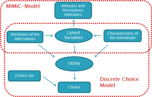
Figure 1 describes the typical structure of a hybrid discrete choice (HDC) model.

Figure 1. Hybrid discrete choice model with latent variables.

It is convenient to estimate the model simultaneously (i.e. MIMIC and discrete choice models jointly) as a sequential estimation may lead to biased results (Bahamonde-Birke and Ortúzar 2014a, 2014b). In this case, the likelihood function takes the following form: (4) $L_q={\int }_{\upsilon }P(y_q|X_q,{\eta }_q;\alpha ,\beta ,{\mathrm{\Sigma }}_U,{\mathrm{\Sigma }}_{\eta })\cdot P(I_q|X_q,\eta ,{\eta }_q^{\ast };\alpha ,\gamma ,{\mathrm{\Sigma }}_I,{\mathrm{\Sigma }}_{\eta })\cdot f({\eta }_q|X_q,{\eta }_q^{\ast };\alpha ,{\mathrm{\Sigma }}_{\eta })\cdot d{\upsilon }_q$(4) where the first part corresponds to the likelihood of the discrete choice component, the second to that of observing the indicators and the third to the distribution of the LV over which the likelihood function must be integrated.

2.1. Categorizing individuals on the basis of unobserved variables

This is not an easy subject (in contrast with observed socio-economic characteristics, such as income or age), as attitudinal variables are not observed and consequently exhibit intrinsic variability (Walker and Ben-Akiva 2002). Under these circumstances, it is not possibly to associate individuals with specific groups, but only to establish a probability that they belong to them. Moreover, as unobserved variables do no exhibit an unequivocal scale, it is not easy to establish thresholds for the categorization and, as such, the process may appear to be somewhat arbitrary. Below we discuss some methods reported in the literature for this purpose, and propose a new method (DCLV) that allows overcoming some of their shortcomings.

2.1.1. Latent classes with psychometric indicators approach (LCPI)

This approach (Hurtubia et al. 2014) does not attempt to categorize individuals on the basis of an HDC and unobserved latent variables per se, but rather to include psychometric indicators into a LC framework, enriching the categorization process. In this structure, class-membership is assumed to depend exclusively on positively observed individual characteristics (X_q ), while the probability of belonging to a certain class is given by a Multinomial Logit (MNL) model. However, as the authors only consider two different classes, their model can also be expressed as an Ordinal Logit model (McCullagh 1980). For the purposes of this work (for comparison reasons), when classes are an expression of an underlying latent variable, the ordinal interpretation seems more appropriate. Then, assuming that the error term follows a Logistic distribution with zero mean and scale parameter λ (fixed without loss of generality), the probability of an individual belonging to a certain class k is given by: (5) $P_{qk}=\frac{1}{e^{\lambda ({\alpha }_X\cdot X_q-{\psi }_T)}+1}-\frac{1}{e^{\lambda ({\alpha }_X\cdot X_q-{\psi }_B)}+1}$(5) where ψ_B and ψ_T represent the lower (bottom) and upper (top) thresholds describing the class, respectively (and must be estimated). The main difference between this approach and the HDC framework, is that here the LV impact only indirectly on the measurement equations. This way, these are just a function of positively observed individual characteristics (X_q ) and the estimated parameters depend on the individual’s LC. Thus, under this approach equation (3) has the following structure: (6) $I_q=X_q\cdot {\gamma }_k+{\varsigma }_q$(6) where γ_k is a LC specific matrix of parameters. As in this case no LV are being considered, equation (1) simply takes the following form: (7) $U_q=X_q\cdot {\beta }_X+{\epsilon }_q$(7) leading to the likelihood function (8): (8) $L_q=\sum _{k}P(y_q|X_q;\alpha ,{\beta }_k,{\mathrm{\Sigma }}_U)\cdot P(I_q|X_q;\alpha ,{\gamma }_k,{\mathrm{\Sigma }}_I)\cdot P_{qk}$(8) where β_k is a LC specific matrix of parameters. Note that while (6) and (7) do not have common parameters, they are connected with each other via (5) as γ_k and β_k are LC-specific. This approach offers computational advantages, as it requires no integration over the domain of the LV.

Nevertheless, despite enriching the categorization process with additional information, the absence of causality assumptions between classes and outcomes in the specification of the model, which is something inherent to all LC models, remains in the LCPI approach.

In contrast with the HDC framework, where it is assumed that the stated indicators are an expression of underlying attitudes or perceptions (and the analyst is forced to make assumptions, specifying a priori, which indicators are going to be explained by which LV), in the LCPI no ex-ante causality assumptions are required (note that these causality assumptions refer to the specification of the model and not to causality per se, which cannot be directly established). Moreover, in most cases the analyst cannot explicitly specify different structures to be tested for the different classes, and the classes are simply defined by the optimization process to improve the likelihood of observing the outcomes. ⁴ As a consequence, in an LCPI structure, the indicators are mainly a tool to improve class-identification (individuals are more or less likely to belong to a certain LC given their stated indicators) and it is not easy for the analyst to guide the model towards identifying a specific unobserved/unobservable trait. Given this inherent difficulty, associating a given latent class with a specific characteristic is mostly done a posteriori after considering the estimated parameters; but this often appears to be a somewhat ad-hoc approach to classify individuals.

Furthermore, as the complex structure of the LCPI framework (requiring the joint consideration of several sets of LC specific measurements equations) is very demanding in terms of data variability, empirical identification problems (Cherchi and Ortúzar 2008) may also arise.

However, it is important to acknowledge that the LCPI framework will offer the best possible adjustment to the data, as LC represent the optimal classification given input and output variables. Thus, it carries the potential to replicate the data more accurately than any other classification approach. But, as previously mentioned, it is challenging for the analyst to elucidate which are the actual underlying behavioural triggers. Nevertheless, when using LC in a confirmatory fashion – rather than in an exploratory fashion – it becomes easier to ascribe a meaning to the identified classes (El Zarwi, Vij, and Walker 2018), although the difficulties to guide the model towards the identification of a specific group remain given the usual impossibility of specifying LC differently (especially when dealing with attitudes or perceptions resulting in systematic taste variations).

Finally, as the approach aims at identifying behavioural groups only (which are of discrete nature), it is not possible to extend it to consider a discrete-continuous treatment of unobserved variables (which may be interesting for the analyst in several instances, for example, when considering missing income data).

2.1.2. Latent variable latent class approach (LVLC)

An alternative approach to classify individuals into distinct behavioural groups, while allowing for the analyst to explicitly specify the links between indicators and latent constructs, is the LVLC method (Hess, Shires, and Jopson 2013; Motoaki and Daziano 2015). It relies on a latent variable η^c (modelled within an HDC framework – (2), (3) and (4)) for the categorization. This way, the likelihood of an individual belonging to a certain class (i.e. being categorized in a certain way) is given by the probability of η^c being smaller (or larger) than a set of thresholds (to be estimated), under a probabilistic categorizing function. ⁵ Basically, it means including η_c into a typical LC framework.

If we assume that the class probability is given by a Logistic function, the likelihood of an individual belonging to a given class can be written as follows (Hess, Shires, and Jopson 2013 ⁶ ): (9) $\begin{array}{l}{P}_{qk}={\displaystyle \frac{1}{e^{\lambda ({\eta }_q^c-{\psi }_T)}+1}}-{\displaystyle \frac{1}{e^{\lambda ({\eta }_q^c-{\psi }_B)}+1}}\\ P_{qk}={\displaystyle \frac{1}{e^{\lambda (X_q\cdot {\alpha }_{Xc}+{\eta }_q^{\ast }\cdot {\alpha }_{\eta c}+{\upsilon }_c-{\psi }_T)}+1}}-{\displaystyle \frac{1}{e^{\lambda (X_q\cdot {\alpha }_{Xc}+{\eta }_q^{\ast }\cdot {\alpha }_{\eta c}+{\upsilon }_c-{\psi }_B)}+1}}\end{array}$(9) Then, the utility functions are given by: (10) $U_q=X_q\cdot {\beta }_{Xk}\cdot +{\eta }_q\cdot {\beta }_{\eta }+{\epsilon }_q$(10) where β_Xk is a LC specific matrix of parameters and η_q is a vector of continuously treated LV. Then, the overall likelihood function for the LVLC framework is given by: (11) $L_q=\sum _k{\int }_{\upsilon }\begin{array}{l}P(y_q|X_q,{\eta }_q;\alpha ,{\beta }_k,{\mathrm{\Sigma }}_U,{\mathrm{\Sigma }}_{\eta })\cdot P(I_q|X_q,\eta ;\alpha ,\gamma ,{\mathrm{\Sigma }}_I,{\mathrm{\Sigma }}_{\eta })\\ \cdot f({\eta }_q|X_q,{\eta }_q^{\ast };\alpha ,{\mathrm{\Sigma }}_{\eta })\cdot d\upsilon \end{array}\cdot P_{qk}$(11) Unfortunately, this approach implies adding the variability associated with the distribution of the categorizing function (or of the LC model, if we approach modelling from this perspective) to the LV’s own error term υ (see [2]). In fact, if just for explanatory purposes we wrote equation (9) in terms of utility functions (which is not entirely appropriate in this case) rather than cumulative probabilities (and considering just the first class, where ψ_B = -∞), we would obtain: (12) $\begin{array}{l}{U}_{\notin k}={\psi }_T\\ U_{\in k}=X\cdot {\alpha }_{Xc}+{\eta }^{\ast }\cdot {\alpha }_{\eta c}+{\upsilon }_c+\epsilon \end{array}$(12) where ε follows a Logistic distribution (alternatively ε could be the difference of two independent and identically distribute EV1 error terms – one of them associated with the upper equation in [12]). From here, it is obvious that by including this stochastic unobserved variable into the LC framework, the analyst is (artificially) imposing that the magnitude of the error term associated with the LV has to be larger when considering it in the classification function than in the measurement equations. The reasons for this relate to the structure of the model: when considering random error terms, their effects are necessarily additive and cannot cancel out (as variances are additive); thus, when considering random disturbances in a model, we must allow for their impact to be zero. However, in the LVLC specification, the modeller considers two additive error terms, the variability of which is, by construction, non-zero.

2.1.3. Direct categorization of individuals on the basis of latent variables approach (DCLV)

To overcome the aforementioned problem in the treatment of the error terms, this paper introduces a new method based on a direct categorization on the basis of LV. It basically consists in associating an individual with a latent class k if a given latent variable η^c falls between a set of thresholds ψ (without using an additional categorizing function). This way, it is possible to establish a probability that a certain individual should be categorized in a given way. Then, it should be possible to estimate the thresholds, and the probability of an individual being categorized in certain fashion (P_qk ) would be given by (13): (13) $\begin{array}{l}{P}_{qk}=P({\psi }_B<{\eta }_q^c<{\psi }_T|s,\alpha ,{\mathrm{\Sigma }}_{\eta })\\ P_{qk}=P(X_q\cdot {\alpha }_{Xc}+{\eta }_q^{\ast }\cdot {\alpha }_{\eta c}+{\upsilon }_q^c<{\psi }_T)-P(X_q\cdot {\alpha }_{Xc}+{\eta }_q^{\ast }\cdot {\alpha }_{\eta c}+{\upsilon }_q^c<{\psi }_B)\end{array}$(13) Note that this approach avoids inducing extra variability into the categorization process (as the LVLC does), because no additional error term is added. Unfortunately, HDC models do not have a closed form and, therefore, they are normally estimated using simulation methods (Ben-Akiva et al. 2002; Bierlaire 2003). This way, we do not observe a continuous distribution for the error term υ of the latent variable η^c , but a set of stochastic (or pseudo-stochastic) draws describing a probability function. As a consequence, discontinuity issues arise, the threshold cannot be estimated and perfect convergence of the algorithm is not theoretically warranted. ⁷

An alternative to overcome this problem would be to rely on auxiliary variables. First, we define an auxiliary latent variable to be categorized η^a _q , following the exact same specification (i.e. same specification and same parameters) as η^c _q , such that: (14) ${\eta }_q^a=X_q\cdot {\alpha }_Y+{\eta }_q\cdot {\alpha }_{\eta }+{\upsilon }_q^a$(14) Here, the error term υ^a _q may be considered via simulation and, consequentially, η^a _q can be used to compute the probabilities every time the actual numeric and continuous value of η^c _q is required. In turn, to compute the likelihood of being categorized in a given fashion, the actual latent variable η^c _q (i.e. not the auxiliary one η^a _q the error term of which is computed via simulation) is used. If we then impose that the distribution of the error terms υ^a _q and υ^c _q (which is the same by construction) is such that their cumulative distribution function can be represented trough a smooth closed-form expression (defined for all real numbers ⁸ ), the probability that η^c _q be larger than a certain threshold, depicted in (13), is given by a closed-form expression (which allows estimating the thresholds). A convenient assumption satisfying this condition, is to assume an i.i.d. Logistic distribution with zero mean and a given scale parameter (fixed without loss of generality), so that (13) may be as an Ordinal Logit model: (15) $P_{qk}=P({\psi }_B<{\eta }_{{}_q}^c<{\psi }_T|s,\alpha ,\upsilon )=\frac{1}{e^{\lambda (X_q\cdot {\alpha }_{Xc}+{\eta }^{\ast }\cdot {\alpha }_{\eta c}-{\psi }_T)}+1}-\frac{1}{e^{\lambda (X_q\cdot {\alpha }_{Xc}+{\eta }^{\ast }\cdot {\alpha }_{\eta c}-{\psi }_B)}+1}$(15) This formulation leads to a likelihood function of the form: (16) $L_q=\sum _k{\int }_{\upsilon }\begin{array}{l}P(y_q|X_q,{\eta }_q,{\eta }_q^a;\alpha ,{\beta }_k,{\mathrm{\Sigma }}_U,{\mathrm{\Sigma }}_{\eta })\cdot P(I_q|X_q,{\eta }_q,{\eta }_q^a;\alpha ,\gamma ,{\mathrm{\Sigma }}_I,{\mathrm{\Sigma }}_{\eta })\\ \cdot f({\eta }_q|X_q,{\eta }_q^{\ast };\alpha ,{\mathrm{\Sigma }}_{\eta })\cdot d\upsilon \end{array}\cdot P_{qk}$(16) Note that the formulation of (16) is exactly the same as (11) except that the integral is only affected by η^a _q , while P_qk is only a function of η^c _q .

Finally, it is important to note that assuming i.i.d. terms for υ^c _q and υ^a _q implies that all observations are independent. This may appear to be a rather innocuous limitation, but has major implications when working with panel data (or pseudo-panel data as in stated choice experiments), as, in this case, integration over the domain of the latent variables should be performed at an individual level (Ortúzar and Willumsen 2011, Chapter 8). This problem can be reduced by including random panel effects into both η^c _q and η^a _q , but at least a proportion of variability would still be independent.

Another way to overcome the problem, while using the DCLV approach (but not auxiliary variables), would be to assume a distribution for the error terms such that a non-simulated-based estimation could be performed (e.g. as in the MACML approach of Bhat 2011). Another inconvenient is related with the non-monotonicity of the categorizing function. This leads to the existence of local optima and therefore the categorization’s threshold will depend on the starting value. Nevertheless, this problem is common to all latent class approaches.

2.2. Empirical issues

As previously mentioned, the modeller can rely on a different number of categories to represent the intensity of the LV (or even on the combination of different categorized LV, akin to constructing classes combining different categorical socioeconomic variables, such as income or education level). To establish the optimal number of categories, the analyst may estimate models considering different numbers of classes. To judge if including an additional category improves the fit, the analyst can rely on the likelihood-ratio (LR) test (Ortúzar and Willumsen 2011), bootstrapping, or information criteria such as the AIC or BIC (Nylund et al.,2007).

Note that when working with several categories, the first and/or last thresholds may tend to diverge, so individuals categorized into the extreme categories would be associated with the tails of the distribution. Even though, this could improve the model’s goodness-of-fit, it may not translate into a better model, as these categories would just characterize outliers (i.e. this is equivalent to selecting a category with two or three individuals when categorizing on the basis of observed socioeconomic variables). In this case it may be advisable to fix exogenously the first and/or last thresholds.

Even though fixing a threshold a priori is an arbitrary decision (which again, must be in accordance with underlying theory), relying on the following heuristic may be useful: (i) estimate a model considering the desired number of categories plus one. (ii) ignore the first (or last) calibrated threshold and estimate a new model considering the desired number of categories; in this case, the first (or last) threshold is fixed at the level of the second (or second from last) estimated threshold in the first model.

Further, and even though in our derivation we considered only the categorization of a single latent variable, it is possible to extend this approach to categorize more variables. That being the case, the categories would be given by the combination of the categorized latent variables. For instance, when considering two categorized latent variables, we would have: (17) $P_k=P({\psi }_{B1}<{\eta }_{c1}<{\psi }_{T1}\wedge {\psi }_{B2}<{\eta }_{c2}<{\psi }_{T2}|s,\alpha ,{\mathrm{\Sigma }}_{\eta })$(17) And if we consider the error terms of both structural equations to be independent, then equation (17) can be written as: (18) $P_k=P_{k1}\cdot P_{k2}=P({\psi }_{B1}<{\eta }_{c1}<{\psi }_{T1}|s,\alpha ,{\mathrm{\Sigma }}_{\eta })\cdot P({\psi }_{B2}<{\eta }_{c2}<{\psi }_{T2}|s,\alpha ,{\mathrm{\Sigma }}_{\eta })$(18) It must be pointed out, however, that establishing categories on the basis of several latent variables may lead to a significant increase in estimation costs.

3. Illustrative examples

To illustrate the analytical considerations made in Section 2, we applied the LVLC and DCLV approaches to empirical data. A fair comparison with the LCPI approach was not possible due to its completely different structure and aims, so our conclusions relating to this approach are based exclusively on the previous theoretical arguments. As classes in the LCPI are defined exclusively to maximize goodness-of-fit, the approach has to be more likely than models estimated according to LV specifications. In fact, a simple LC model (without indicators) would always outperform all competing approaches as, in this case, the LC are defined with the single purpose of maximizing the goodness-of-fit of the observed choices (i.e. having to satisfy jointly both the observed choices and the psychometric indicators, can be understood as a restriction in the definition of the latent classes). This is related with the discussion raised by Vij and Walker (2016): a simple LC model represents the reduced form of both the LVLC and the DCLV (as a LC model is a ML with a discrete mixing distribution). Hence, a LV approach cannot outperform a LC model in terms of fit.

Similarly, the LCPI represents the reduced form of a discrete mixed model maximizing the likelihood associated with the representation of both choices and indicators simultaneously. Imposing any functional form on the way both types of variables are related, necessarily implies a worsening of fit (as it imposes a restriction in the categorization). However, if these functional forms are driven by theory, the model still can offer a better representation of the phenomenon (despite the worst fit). Furthermore, and also akin to the discussion between the HDC models and the reduced ML, the representation based on the LVLC or the DCLV offers significant advantages in terms of behavioural insights.

Both case studies are only intended to serve as illustrative examples of the methodological issues discussed in the previous section. For a deeper discussion on their findings the reader is referred to Bahamonde-Birke and Hanappi (2016; Case 1) or to Bahamonde-Birke et al. (2014; Case 2).

3.1. Case 1 – electromobility in Austria

Our first example comes from the DEFINE project. A web-based survey conducted in Austria during February 2013, considered a stated preference (SP) vehicle purchase experiment set in the context of different electromobility options (Bahamonde-Birke and Hanappi 2016). The discrete choice experiment considered 787 respondents, and used a labelled experimental design, including four alternatives referring to different propulsion technologies: conventional vehicles (CV), plug-in hybrid-electric vehicles (PHEV), hybrid-electric vehicles (HEV) and electric vehicles (EV). Each alternative was described by the following attributes: purchase price (PP), power (PS), fuel costs (FC) and maintenance costs (MC). In addition, the EV were further characterized by the following attributes: full driving range (RA), availability of charging stations (LS) and policy incentives (IM). Charging station availability varied across three categories (low, intermediate and high) and was described qualitatively using a separate pop-up box. Policy incentives included a Park & Ride subscription for one year (IM2), investment subsidies to support private charging stations (IM3), and a one-year-ticket for public transport (IM4).

Additionally, attitudinal indicators related to the degree of agreement with eight different sentences were collected. Bahamonde-Birke and Hanappi (2016) considered the following five of them to construct a latent variable related to the environmental attitude of the individuals: ‘I am an ecologically aware person’ (EcAwareness), ‘I pay attention to regional origins when shopping foods and groceries’ (LocalFood), ‘I buy ecologically friendly products’ (EcoFriendly), ‘Environmental protection measures should be enacted even if they result in job losses’ (Protection) and ‘I pay attention to the CO2 footprint of the products I buy’ (CO2Footprint). The level of agreement was stated using a six-point Likert scale. Table 1 presents an overview of the relevant variables for this study. ⁹

Table 1. Definition of the variables considered in the model. Case 1.

Variable	Definition
MidSkill	Dummy variable indicating a career and technical education.
HighSkill	Dummy variable indicating a college education or higher.
Vienna	Dummy variable indicating a residence in Vienna.
Male	Dummy variable indicating masculine gender.
Old	Dummy variable indicating individuals older than 60 years
MidAge	Dummy variable indicating individuals older than 35 years, but no older than 60 year.
Carsharing	Dummy variable indicating that the individual relies on Car Sharing on a regular basis.
CarUser	Dummy variable indicating that the individual drives to their main occupational activity on a regular basis.
PP	Purchase price in €.
FC, MC	Fuel and maintenance cost in € / 100 km., respectively.
PS	Power of the engine in hp.
RA	Driving range in km.
IM2, IM3, IM4	Dummy variables indicating the execution of the respective policy incentive.
LSMid, LSHigh	Dummy variables indicating medium or high availability of loading stations for EV.
LV Green	Latent variable Green accounting for environmental awareness.
DLV Green	Discretized latent variable Green accounting for individuals with high environmental awareness.
EcAwareness	Attitudinal Indicator for ‘I am an ecologically aware person’.
LocalFood	Attitudinal Indicator for ‘I pay attention to regional origins when shopping foods and groceries’.
EcoFriendly	Attitudinal Indicator for ‘I buy ecologically friendly products’.
Protection	Attitudinal Indicator for ‘Environmental protection measures should be enacted even if they result in job losses’.
CO2Footprint	Attitudinal Indicator for ‘I pay attention to the CO2 footprint of the products I buy’.

Using PythonBiogeme (Bierlaire 2003), we estimated two models following both approaches presented in the previous section. Taking advantage of having just one latent variable, the log-likelihood was computed using numerical integration.

The latent variable (LV Green) accounts for environmental awareness and was discretized into two levels. Hence, the dichotomous latent variable DLV Green (taking a value of one if LV Green is larger than a threshold to be estimated and zero otherwise) defines the two different latent classes (note that the inclusion of a single dichotomous variable allows estimating different parameters for the entire class). The inclusion of the aforementioned dummy variable, allows us to differentiate between a latent class of more environmentally concerned individuals and a latent class of less environmentally concerned individuals.

The specification of the utility functions of both latent classes is basically the same, apart from the inclusion of DLV Green in association with the variables HEV, PHEV and BEV, which allows for estimating class-specific parameters for the latter. While usually LC models consider the estimation of a different sets of parameters for each class, here we imposed the restriction that most parameters were generic across classes and only one parameter was different. The reason was that the empirical exercise had an illustrative purpose and having both classes differing in only one parameter facilitated the illustration of the differences. However, note that considering a full-set of class-specific parameters is not only possible, but potentially one of the main advantages of the approach compared with HDC models with only continuous LV, as it easily allows addressing systematic taste variations among classes.

In this application, it was only possible to identify two statistically different classes and the model results are presented in Table 2. The t-test for statistical significance are presented in parenthesis and the log-likelihood for the overall model, as well as for the discrete choice (DC) component only, are also reported (the results for the measurement equations are shown in the appendix). The indicators were considered discrete outputs following an Ordered Logit model approach.

Table 2. Parameter estimates. Case 1.

Variable	Equation	LVLC		DCLV
Vienna	S.E. LV Green	−0.333	(−2.56)	−0.182	(−1.71)
Male	S.E. LV Green	−0.597	(−5.58)	−0.587	(−5.74)
HighSkill	S.E. LV Green	1.05	(6.16)	0.879	(5.89)
MidSkill	S.E. LV Green	0.536	(3.85)	0.477	(3.72)
Old	S.E. LV Green	1.09	(7.18)	0.955	(6.67)
MidAge	S.E. LV Green	0.657	(5.15)	0.615	(5.14)
Carsharing	S.E. LV Green	1.33	(4.9)	0.988	(4.99)
CarUser	S.E. LV Green	−0.567	(−5.53)	−0.474	(−5.7)
Threshold	C.F	3.76	(5.27)	2.23	(7.18)
Scale Parameter	C.F	0.538	(5.06)	1	(fixed)
ASC_CV	Utility CV	0	(fixed)	0	(fixed)
ASC_HEV	Utility HEV	−0.0165	(−0.07)	0.0945	(0.41)
ASC_PHEV	Utility PHEV	−0.235	(−0.94)	−0.207	(−0.88)
ASC_EV	Utility EV	−1.09	(−2.65)	−0.982	(−2.36)
PP	Utility CV	−1.21	(−7.92)	−1.27	(−9.07)
PP	Utility HEV	−1.8	(−22.39)	−1.79	(−22.85)
PP	Utility PHEV	−1.76	(−19.94)	−1.77	(−20.48)
PP	Utility EV	−1.66	(−9.79)	−1.73	(−10.69)
MC	Utility CV, HEV, PHEV, EV	−21.1	(−9.32)	−20.6	(−9.6)
FC	Utility CV, HEV, PHEV, EV	−21.4	(−14.96)	−20.7	(−15.87)
PS	Utility CV	0.0327	(5.22)	0.0341	(5.74)
PS	Utility HEV	0.0353	(7.18)	0.0348	(7.37)
PS	Utility PHEV	0.0354	(7.2)	0.0367	(7.5)
PS	Utility EV	−0.000269	(−0.05)	−0.000232	(−0.05)
PS * Male	Utility CV	−0.019	(−4.14)	−0.0195	(−4.21)
PS * Male	Utility HEV	−0.0164	(−3.38)	−0.0164	(−3.38)
PS * Male	Utility PHEV	−0.0155	(−3.16)	−0.0162	(−3.26)
PS * Male	Utility EV	−0.00302	(−0.55)	0.000491	(0.09)
MidAge	Utility HEV	−0.266	(−2.5)	−0.287	(−2.65)
MidAge	Utility PHEV	−0.383	(−3.46)	−0.374	(−3.48)
MidAge	Utility EV	−0.784	(−4.55)	−0.946	(−4.91)
Old	Utility HEV	−1.18	(−5.82)	−1.19	(−5.63)
Old	Utility PHEV	−1.44	(−6.24)	−1.35	(−6.07)
Old	Utility EV	−2.55	(−9.02)	−2.88	(−8.77)
DLV Green	Utility HEV	3.48	(6.86)	3.19	(6.56)
DLV Green	Utility PHEV	3.25	(6.08)	2.71	(4.84)
DLV Green	Utility EV	5.77	(8.5)	5.89	(9.83)
RA	Utility EV	0.00444	(6.25)	0.00459	(6.81)
LSMid	Utility EV	0.0121	(0.07)	0.0426	(0.25)
LSHigh	Utility EV	0.661	(4.22)	0.71	(4.43)
IM3	Utility EV	0.306	(2.19)	0.305	(2.14)
Log-likelihood
Overall Model		−16,177.759		−16,169.571
Log-likelihood
DC Component		−6,612.876		−6,605.847

The differences between the parameter values obtained following both approaches are not large and many are not statistically different. This applies to all parameters of the structural and measurement equations as well as the utility functions, with the exception of the threshold parameter of the categorizing function. This last parameter evidently exhibits a different value, as the LVLC approach is associated, by construction, with a larger error and a wider distribution, implying that the threshold must be located further away from the expected value to capture the behaviour of the same individuals.

The DCLV approach exhibits a better goodness-of-fit than the LVLC, despite the fact that the latter has one extra degree-of-freedom (providing further evidence about the incorrect error treatment in the LVLC). This result is in accordance with our expectations, as the LVLC considers an additional non-zero error component, which is unnecessary for model estimation. Along this line, the improvement in goodness-of-fit is mostly explained by the discrete choice component, and this is based on the fact that the categorization (and its additional error term) affects only the utility functions.

3.2. Case 2 – modal choice in Germany

In this SP experiment respondents were asked to choose between different interurban public transport alternatives in Germany (regional and intercity trains, and interurban coaches). The experiment was carried out in three waves, contacting students and employees of two universities in Berlin as well as employees of member institutions of the Leibniz-Gemeinschaft (Bahamonde-Birke et al. 2014). Respondents were required to choose between a first pivotal alternative, representing a trip previously described, and a new one. Alternatives were described in terms of their travel time, fare, number of transfers, safety level and mode of transport: regional trains (RE), intercity trains (FVZ) and coaches (LB).

The original study considered several indicators, associated with different and complex latent variables. For the purposes of this work we only considered one LV (TrainFan), associated with the following two indicators: ‘Investing on the development of high-speed trains should be encouraged’ (HSTrains) and ‘New high-speed rail lines should be built’ (RailLines). Originally, the indicators were stated in a 10-point Likert scale. For computational simplicity, in this application we reduced it to only five, aggregating consecutive levels. Table 3 presents an overview of the variables considered.

Table 3. Definition of the variables considered in the model. Case 2.

Variable	Definition
Inertia	Dummy variable taking the value of one for the status quo alternative.
FVZ	Dummy variable taking the value of one if the alternative considers the use of intercity trains.
RE	Dummy variable taking the value of one if the alternative considers the use of regional trains.
LB	Dummy variable taking the value of one if the alternative considers the use of coaches.
Old	Dummy variable indicating individuals older than 50 years.
Bahncard	Dummy variable indicating ownership of a Deutsche Bahn yearly discount card.
Woman	Dummy variable indicating feminine gender.
VeryLowIncome	Dummy variable indicating a net income under 700€ p.m.
LowIncome	Dummy variable indicating a net income between 700€ and 1,500€ p.m.
MiddleIncome	Dummy variable indicating a net income between 1,500€ and 2,500€ p.m.
HighIncome	Dummy variable indicating a net income over 2,500€ p.m.
Price	Travel fare in €.
TravelTime	Travel time in minutes.
Transfers	Number of transfers.
SafetyLevel	Number of severely injured passengers and the number of fatalities in the overall network over a year.
LV TrainFan	Latent variable TrainFan.
DLV TrainFan	Discretized latent variable accounting for individuals with high affinity for trains (two categories only).
DLV TrainFan2	Discretized latent variable accounting for individuals with medium affinity for trains (3 categories only).
DLV TrainFan3	Discretized latent variable accounting for individuals with high affinity for trains (3 categories only).
HSTrains	Attitudinal Indicator for ‘Investing on the development of high-speed trains should be encouraged’.
RailLines	Attitudinal Indicator for ‘New high-speed rail lines should be built’.

As in the previous case, the LV TrainFan was used to construct the latent classes with the dichotomous variable DLV TrainFan taking a positive value if LV TrainFan was larger than a threshold. The only difference in the specification of the utility functions of both classes is that the valuation of the alternative FVZ is class-specific (as it interacts with DLV TrainFan).

Models following the LVLC and DCLV approaches were again estimated using PythonBiogeme and considering numerical integration for the computation of the likelihood function. Indicators were considered discrete outcomes (OLM). Table 4 presents the results for both models (again only two statistically different classes were identified). The structure of the table is the same as in the previous case (results for the measurement equations are presented, once more, in the appendix).

Table 4. Parameter estimates. Case 2.

Variable	Equation	LVLC		DCLV
Old	S.E. LV TrainFan	0.207	(0.36)	−0.093	(−0.41)
Bahncard	S.E. LV TrainFan	0.684	(5.41)	0.673	(5.46)
Woman	S.E. LV TrainFan	−0.686	(−5.64)	−0.663	(−5.75)
MiddleIncome	S.E. LV TrainFan	0.368	(3.19)	0.426	(3.24)
HighIncome	S.E. LV TrainFan	0.515	(2.53)	0.606	(2.82)
Threshold	C.F	0.622	(1.44)	−0.346	(−0.59)
Scale Parameter	C.F	10	(fixed)	1	(fixed)
Inertia	Utility Alternative 1	0.336	(13.48)	0.345	(13.48)
FVZ	Utility Alternative 1 and 2	0	(fixed)	0	(fixed)
LB	Utility Alternative 1 and 2	−1.17	(−12.65)	−0.559	(−12.62)
RE	Utility Alternative 1 and 2	−0.167	(−9.59)	0.448	(9.52)
Travel Time	Utility Alternative 1 and 2	−1.49	(−26.57)	−1.56	(−26.57)
Ln(Price) * Very Low Income	Utility Alternative 1 and 2	−5.29	(−31.91)	−5.41	(−31.9)
Ln(Price) * Low Income	Utility Alternative 1 and 2	−4.7	(−26.28)	−4.85	(−26.26)
Ln(Price) * Middle Income	Utility Alternative 1 and 2	−3.63	(−14.98)	−3.8	(−15)
Ln(Price) * High Income	Utility Alternative 1 and 2	−2.54	(−7.81)	−2.67	(−7.84)
Safety Level	Utility Alternative 1 and 2	−0.00374	(−4.59)	−0.00408	(−4.59)
Transfers	Utility Alternative 1 and 2	−0.446	(−18.25)	−0.46	(−18.25)
FVZ * DLV TrainFan	Utility Alternative 1 and 2	0.716	(4.93)	1.42	(5.27)
Log-likelihood
Overall Model		−10,543.642		−10,535.42
Log-likelihood
DC Component		−7,461.029		−7,453.871

While in Case 1 all estimators (apart from the threshold) were not statistically different in both models, in Case 2 the parameters associated with the discretized LV are significantly different. As the discretized LV is considered in conjunction with the modal parameter of the intercity trains, it also affects the remaining modal parameters. This difference may be attributed to the fact that changing the distribution (the variability) of the categorizing function may allow for identifying different groups of people. In fact, taking a look at the threshold parameters, it seems (accounting for the wider variability of the LVLC) that the thresholds have been set at a different level.

Notoriously in this case, when following the LVLC approach, the scale parameter λ of the categorizing function diverged (at least in computational terms). For that reason, it was necessary to fix it as 10 (larger values led to computational problems when computing the Fisher information matrix, but neither the estimates nor the final value of the log-likelihood were significantly affected).

The DCLV approach offered, again, a better adjustment than the LVLC model to the data; this may be mainly related to a better explanation of the discrete choices. Interestingly in this case, the scale parameter of the LVLC model suggests that the categorizing function should be as close to a Dirac delta function (Dirac 1958) as possible. In this limit, the LVLC model would collapse to the DCLV. Nevertheless, it is not possible to achieve this limit (or get close to it) due to computational limitations (variable overflow); therefore, it is impossible to get rid of the error induced through the LVLC approach.

In both cases studies we were only able to identify two statistically different classes; notwithstanding, and for illustrative purposes, we also present here a model considering three classes. In this case, the LV TrainFan was used to construct the dichotomous variables DLV TrainFan1 – identifying a latent class of individuals moderately supportive of trains, and DLV TrainFan2 – identifying a latent class of individuals highly supportive of trains. The third latent class corresponded to individuals for which none of the DLV are active, and identifies individuals with a low support for trains. The difference between the three latent classes is only the valuation of intercity trains (FVZ). In this case, it was necessary to fix the first threshold following the heuristic proposed in section 2 (for that purpose, a model considering four classes was previously calibrated). The results are presented in Table 5 (we only include the DCLV model, as fixing the first threshold does not allow for a fair comparison between both approaches ¹⁰ ).

Table 5. Parameter estimates. Case 2. Three categories.

Variable	Equation	DCLV
Old	S.E. LV TrainFan	−0.107	(−0371)
Bahncard	S.E. LV TrainFan	0.648	(6.28)
Woman	S.E. LV TrainFan	−0.664	(−6.27)
MiddleIncome	S.E. LV TrainFan	0.426	(3.97)
HighIncome	S.E. LV TrainFan	0.603	(3.40)
Threshold1	C.F	−0.761	(fixed)
Threshold2	C.F	0.442	(0.42)
Scale Parameter	C.F	1	(fixed)
Inertia	Utility Alternative 1	0.344	(13.17)
FVZ	Utility Alternative 1 and 2	0	(fixed)
LB	Utility Alternative 1 and 2	−0.447	(−1.77)
RE	Utility Alternative 1 and 2	0.559	(2.42)
Travel Time	Utility Alternative 1 and 2	−1.55	(−25.01)
Ln(Price) * Very Low Income	Utility Alternative 1 and 2	−5.40	(−30.42)
Ln(Price) * Low Income	Utility Alternative 1 and 2	−4.85	(−25.17)
Ln(Price) * Middle Income	Utility Alternative 1 and 2	−3.81	(−14.86)
Ln(Price) * High Income	Utility Alternative 1 and 2	−2.68	(−7.92)
Safety Level	Utility Alternative 1 and 2	−0.00407	(−4.77)
Transfers	Utility Alternative 1 and 2	−0.459	(−17.90)
FVZ * DLV TrainFan2	Utility Alternative 1 and 2	1.03	(1.76)
FVZ * DLV TrainFan3	Utility Alternative 1 and 2	1.63	(5.56)
Log-likelihood
Overall Model		−10,534.62
Log-likelihood
DC Component		−7,453.107

As can be observed, besides the latent class specific parameters, the remaining estimates do not divert significantly from the previous model. Further, including a third class does not represent a statistical improvement. In fact, performing a likelihood-ratio test between both DCLV models yields: (19) $D=-2\cdot (\mathrm{\Delta }L)=1.6<{\chi }_{1;90\mathrm{\%}}^2=2.706$(19) As a consequence, it is not possible to reject the null hypothesis of equality between both models even at a significance level of 10%. Hence, only two categories should be considered.

4. Conclusions

Classifying individuals, based on their unobserved characteristics, offers significant opportunities from a modelling perspective, as well as a chance to gain significant insights into their decision-making process. Nowadays, the dominant approach to probabilistically categorize individuals based on unobserved characteristics is the latent class approach. However, this method has been subject to criticism due to the intrinsic difficulties associated with linking latent classes (LC), as identified by the model, with behavioural elements. This criticism may be overruled when LC are used for identifying objective properties (such as missing information, lexicographic respondents, etc.), and the analyst can specify different utility functions for different LC, aiding (and guiding) their identification. However, when attempting to model attitudes, perceptions, and other latent characteristics of individuals, the analyst cannot control or guide the identification process of the latent classes by using different (class-specific) specifications. Additionally, the classical latent class approach does not take advantage of additional information, such as the existence of psychometric indicators.

In this work, we explored three ways to improve the categorization of individuals. First, we considered the LCPI approach, which improves the categorization by considering exogenous information (psychometric indicators), but it is guilty of the same problem associated with the LC models described previously. Note that, by definition, this approach should offer a superior goodness-of-fit than alternative approaches, as the class-membership function is built to maximize fit and not to satisfy a given specification. This fact is a double-edged sword, as, on the one hand, it may offer more insights into the actual underlying decision-making process, but it also poses significant difficulties for the analyst in terms of testing a specific theory or identifying a given behavioural pattern.

In the second place, we examined the LVLC approach, which combines the HDC and LC frameworks, by considering latent variables into the class-membership function. Unfortunately, this approach is guilty of an incorrect specification of the error terms, leading to an artificial decrease in the model’s adjustment. Finally, we proposed an alternative way to attempt a direct categorization of individuals based on latent variables (DCLV). This approach overcomes the error issues of the LVLC.

We further illustrated the differences between the LVLC and DCLV approaches with the help of two case studies (we did not consider the LCPI approach, as given the different nature of the models no fair comparison was possible). In the first example, we could not establish the existence of significant differences in the estimated parameters (aside from the threshold parameter). However, in the second example, the differences in variability of the class-membership function led to a different categorization. In line with our expectations, the DCLV approach offered a superior goodness-of-fit than the LVLC (even though the latter had one extra degree-of-freedom); this is due to the incorrect specification of the error terms. The improvements in goodness-of-fit were mainly explained by a better adjustment of the discrete choice component.

Based on our theoretical analysis and empirical results, we recommend the DCLV approach over the LVLC method. It offers a consistent treatment of the error term, per underlying theory, and also offers a better performance in terms of goodness-of-fit. No definite recommendations can be made regarding the use of the DCLV or LCPI approaches, as both respond to different mechanisms; however, if the modeller aims at testing a specific attitudinal or perceptual characteristic, the DCLV offers significant advantages, as it facilitates specifying the required structure to be tested, and therefore, the identification of the latent construct.

Future research should aim at establishing for which kind of LV and latent phenomena a categorical non-parametric treatment offers significant advantages over continuous parametric treatments. We know that a non-linear effect can be assumed (as done in this work) based on theoretical considerations. It would be advantageous to establish which kind of latent phenomena are unlikely to be accurately captured by parametric representations (at least regarding their impact on utility functions) and which phenomena can eventually be approximated using parametric representations, on an empirical basis. Furthermore, future research should be conducted to evaluate the use of non-simulated estimation techniques to allow for more flexible error term structures in the context of the DCLV.

Acknowledgments

This paper is partially based on scientific work done during the DEFINE (Development of an Evaluation Framework for the Introduction of Electromobility) project. We gratefully acknowledge the funding for DEFINE (https://www.ihs.ac.at/projects/define/) as part of the ERA-NET Plus Electromobility+ call by the EU-Commission and national funding institutions: the Ministry for Transport, Innovation and Technology (Austria), the Federal Ministry of Transport and Digital Infrastructure, formerly Federal Ministry for Transport, Building and Urban Development (Germany), and the National Centre for Research and Development (Poland). We are also grateful to the Institute in Complex Engineering Systems (CONICYT: FB0816), the BRT+ Centre of Excellence funded by the Volvo Research and Educational Foundations, the Alexander von Humboldt Foundation and the Centre for Sustainable Urban Development, CEDEUS (Conicyt/Fondap/15110020). The authors would also like to thank Prof. Michel Bierlaire and five anonymous referees for their useful comments and insights on an earlier version of the paper. All errors are the authors’ sole responsibility.

Disclosure statement

No potential conflict of interest was reported by the author(s).

Notes

1 Modellers mostly use psychometric data to target unobserved/unobservable characteristics of the individuals, such as attitudes or perceptions, the aim of this work. Notwithstanding, they can also use the HDC framework to address other kinds of unobserved/unobservable information of the individuals or the alternatives. In this case, the indicator does not necessarily have to be psychometric data.

2 Even though Walker and Ben-Akiva (2002) postulate a potential link between both components, they did not address it in their work.

3 We use the same matrix of variables X_q in all equations of the paper for notational purposes. It does not imply that all columns of X_q would necessarily impact the outcome. The explicit inclusion of η_q * in (2) simply acknowledges the fact that the structural equations may be subject to endogeneity. When considering a set of simultaneous structural equations, identifiability must be established on a case-by-case basis.

4 Notorious exceptions of the former would be given by situations when LC are used to test the availability of a given alternative (classical use of the LC framework), or when one class is expected to ignore a given attribute (lexicographic preferences), where the modeller indeed specifies the utility functions differently. However, when dealing with attitudes or perceptions that would result in systematic taste variations, the modeller cannot specify the structure differently in most cases, as the difference between classes is merely given by different values for the estimators.

5 Note that Hess, Shires, and Jopson (2013) just considered two classes, not specifying whether they were dealing with a MNL or an Ordinal model (as both specifications are equivalent for two classes). As we aim at latent classes as an expression of an underlying latent variable, we extended their framework as an Ordinal model. This extension does not affect the assessment of the model.

6 In their original specification, Hess, Shires, and Jopson (2013) multiplied η_c by a parameter to be estimated and fixed (λ); however, it is easy to see that both specifications are equivalent.

7 When considering the model sequentially by integrating over the domain of the LV perfect convergence is achieved, but the threshold remains unidentified and must be fixed a priori (Bahamonde-Birke et al., 2017).

8 Just in the case of the LV to be discretized. The errors of any other LV may follow any desired distribution.

9 Bahamonde-Birke and Hanappi (2016) considered further variables and estimated more involved models than those considered in this study. For the purposes of this work, this specification was considered appropriate, as additional complexity would only add noise and computational complexity to our analysis.

10 Given their different structure, the heuristic value used in both models would be necessarily different. While the difference is indeed small, it does not allow for a fair comparison.

Appendix 1. Parameter estimates for the measurement equations. Case 1.

Table

Variable	Equation	LVLC		DCLV
Scale Parameter	M.E. EcAwareness	0.959	(16.14)	0.954	(16.1)
Threshold 1	M.E. EcAwareness	−3.25	(−15.18)	−3.18	(−15.29)
Threshold 2	M.E. EcAwareness	0.0152	(0.09)	0.0719	(0.42)
Threshold 3	M.E. EcAwareness	3.05	(12.85)	3.1	(13.22)
Threshold 4	M.E. EcAwareness	5.06	(14.74)	5.1	(14.9)
Threshold 5	M.E. EcAwareness	7.01	(12.11)	7.05	(12.16)
Scale Parameter	M.E. LocalFood	1.18	(14.89)	1.22	(14.89)
Threshold 1	M.E. LocalFood	−1.76	(−9.58)	−1.68	(−9.51)
Threshold 2	M.E. LocalFood	0.655	(3.74)	0.692	(4.11)
Threshold 3	M.E. LocalFood	2.59	(12.3)	2.59	(12.79)
Threshold 4	M.E. LocalFood	4.23	(15.2)	4.2	(15.63)
Threshold 5	M.E. LocalFood	7.17	(10.56)	7.09	(10.7)
Scale Parameter	M.E. EcoFriendly	0.988	(15.94)	1.02	(16.06)
Threshold 1	M.E. EcoFriendly	−2.68	(−12.98)	−2.58	(−13.01)
Threshold 2	M.E. EcoFriendly	−0.727	(−4.12)	−0.664	(−3.92)
Threshold 3	M.E. EcoFriendly	1.28	(6.9)	1.3	(7.32)
Threshold 4	M.E. EcoFriendly	2.88	(12.85)	2.88	(13.32)
Threshold 5	M.E. EcoFriendly	6.77	(12.65)	6.69	(12.87)
Scale Parameter	M.E. Protection	0.442	(13.06)	0.446	(13.05)
Threshold 1	M.E. Protection	−7.7	(−13.42)	−7.59	(−13.39)
Threshold 2	M.E. Protection	−3.33	(−11.57)	−3.25	(−11.54)
Threshold 3	M.E. Protection	1.3	(5.53)	1.34	(5.83)
Threshold 4	M.E. Protection	4.12	(10.97)	4.14	(11.15)
Threshold 5	M.E. Protection	8.04	(11.84)	8.03	(11.91)
Scale Parameter	M.E. CO2Footprint	0.951	(16.84)	0.95	(16.77)
Threshold 1	M.E. CO2Footprint	−4.39	(−17.52)	−4.32	(−17.61)
Threshold 2	M.E. CO2Footprint	−1.92	(−10.27)	−1.86	(−10.29)
Threshold 3	M.E. CO2Footprint	0.276	(1.56)	0.329	(1.92)
Threshold 4	M.E. CO2Footprint	1.89	(9.4)	1.93	(9.85)
Threshold 5	M.E. CO2Footprint	5.31	(14.73)	5.35	(14.89)

Appendix 2. Parameter estimates for the measurement equations. Case study 2.

Table

Variable	Equation	LVLC		DCLV
Scale Parameter	M.E. HSTrains	1.13	(8.48)	1.09	(7.6)
Threshold 1	M.E. HSTrains	−3.74	(−13.3)	−3.77	(−12.42)
Threshold 2	M.E. HSTrains	−2.21	(−11.8)	−2.21	(−11.3)
Threshold 3	M.E. HSTrains	−0.179	(−1.47)	−0.16	(−1.37)
Threshold 4	M.E. HSTrains	1.43	(10.12)	1.47	(10.56)
Scale Parameter	M.E. RailLines	2.03	(3.9)	2.23	(2.84)
Threshold 1	M.E. RailLines	−2.83	(−12.73)	−2.74	(−11.66)
Threshold 2	M.E. RailLines	−1.5	(−10.01)	−1.44	(−9.44)
Threshold 3	M.E. RailLines	0.0287	(0.26)	0.0539	(0.53)
Threshold 4	M.E. RailLines	1.4	(9.91)	1.4	(9.81)

Appendix 3. Parameter estimates for the measurement equations. Case study 2. Three categories.

Table

Variable	Equation	DCLV
Scale Parameter	M.E. HSTrains	1.09	(7.44)
Threshold 1	M.E. HSTrains	−3.77	(−12.25)
Threshold 2	M.E. HSTrains	−2.21	(−11.18)
Threshold 3	M.E. HSTrains	−0.157	(−1.36)
Threshold 4	M.E. HSTrains	1.47	(10.58)
Scale Parameter	M.E. RailLines	2.26	(2.72)
Threshold 1	M.E. RailLines	−2.73	(−11.49)
Threshold 2	M.E. RailLines	−1.43	(−9.33)
Threshold 3	M.E. RailLines	0.057	(0.57)
Threshold 4	M.E. RailLines	1.4	(9.74)

References

- Ashok, K. , W. Dillon , and S. Yuan . 2002. “Extending Discrete Choice Models to Incorporate Attitudinal and Other Latent Variables.” Journal of Marketing Research 39: 31–46. doi: https://doi.org/10.1509/jmkr.39.1.31.18937
- Bahamonde-Birke, F. J. , and T. Hanappi . 2016. “The Potential of Electromobility in Austria: Evidence from Hybrid Choice Models Under the Presence of Unreported Information.” Transportation Research Part A: Policy and Practice 83: 30–41.
- Bahamonde-Birke, F. J. , U. Kunert , H. Link , and J. de D. Ortúzar . 2014. “Bewertung der Angebotsmerkmale des Personenfernverkehrs vor dem Hintergrund der Liberalisierung des Fernbusmarktes.” Zeitschrift für Verkehrswissenschaft 85 (2): 107–123.
- Bahamonde-Birke, F. J. , U. Kunert , H. Link , and J. de D. Ortúzar . 2017. “About Attitudes and Perceptions – Finding the Proper Way to Consider Latent Variables in Discrete Choice Models.” Transportation 44: 475–493. doi: https://doi.org/10.1007/s11116-015-9663-5
- Bahamonde-Birke, F. J. , and J. de D. Ortúzar . 2014a. “On the Variability of Hybrid Discrete Choice Models.” Transportmetrica A: Transport Science 10 (1): 74–88. doi: https://doi.org/10.1080/18128602.2012.700338
- Bahamonde-Birke, F. J. , and J. de D. Ortúzar . 2014b. “Is Sequential Estimation a Suitable Second Best for Estimation of Hybrid Choice Models?” Transportation Research Record: Journal of the Transportation Research Board 2429: 51–58. doi: https://doi.org/10.3141/2429-06
- Ben-Akiva, M. , and B. Boccara . 1995. “Discrete Choice Models with Latent Choice Sets.” International Journal of Research in Marketing 12: 9–24. doi: https://doi.org/10.1016/0167-8116(95)00002-J
- Ben-Akiva, M. , D. McFadden , K. Train , J. Walker , C. Bhat , M. Bierlaire , D. Bolduc , et al. 2002. “Hybrid Choice Models: Progress and Challenges.” Marketing Letters 13: 163–175. doi: https://doi.org/10.1023/A:1020254301302
- Bhat, C. R. 2011. “The Maximum Approximate Composite Marginal Likelihood (MACML) Estimation of Multinomial Probit-Based Unordered Response Choice Models.” Transportation Research Part B: Methodological 45 (7): 923–939. doi: https://doi.org/10.1016/j.trb.2011.04.005
- Bierlaire, M. 2003. “BIOGEME: A Free Package for the Estimation of Discrete Choice Models.” 3rd Swiss Transportation Research Conference , Ascona, Switzerland.
- Bujosa, A. , A. Riera , and R. L. Hicks . 2010. “Combining Discrete and Continuous Representations of Preference Heterogeneity: A Latent Class Approach.” Environmental and Resource Economics 47 (4): 477–493. doi: https://doi.org/10.1007/s10640-010-9389-y
- Cherchi, E. , and J. de D. Ortúzar . 2008. “Empirical Identification in the Mixed Logit Model: Analysing the Effect of Data Richness.” Networks and Spatial Economics 8: 109–124. doi: https://doi.org/10.1007/s11067-007-9045-4
- Chia-Jung, C. , and C. Pei-Chun . 2014. “Preferences and Willingness to Pay for Green Hotel Attributes in Tourist Choice Behaviour: The Case of Taiwan.” Journal of Travel & Tourism Marketing 31: 937–957. doi: https://doi.org/10.1080/10548408.2014.895479
- DeSarbo, W. S. , V. Ramaswamy , and S. H. Cohen . 1995. “Market Segmentation with Choice-Based Conjoint Analysis.” Marketing Letters 6: 137–147. doi: https://doi.org/10.1007/BF00994929
- Dirac, P. 1958. The Principles of Quantum Mechanics . Oxford : Clarendon Press.
- Domencich, T. , and D. McFadden . 1975. Urban Travel Demand – A Behavioural Analysis . Oxford : North Holland Publishing.
- El Zarwi, F. , A. Vij , and J. L. Walker . 2018. “A Discrete Choice Framework for Modelling and Forecasting the Adoption and Diffusion of New Transportation Services.” Transportation Research Part C: Emerging Technologies 79: 207–223. doi: https://doi.org/10.1016/j.trc.2017.03.004
- Hess, S. , and N. Beharry-Borg . 2012. “Accounting for Latent Attitudes in Willingness-to-Pay Studies: The Case of Coastal Water Quality Improvements in Tobago.” Environmental and Resource Economics 52: 109–131. doi: https://doi.org/10.1007/s10640-011-9522-6
- Hess, S. , J. Shires , and A. Jopson . 2013. “Accommodating Underlying Pro-Environmental Attitudes in a Rail Travel Context: Application of a Latent Variable Latent Class Specification.” Transportation Research Part D: Transport and Environment 25: 42–48. doi: https://doi.org/10.1016/j.trd.2013.07.003
- Humlum, M. K. , K. J. Kleinjans , and H. S. Nielsen . 2012. “An Economic Analysis of Identity and Career Choice.” Economic Inquiry 50: 39–61. doi: https://doi.org/10.1111/j.1465-7295.2009.00234.x
- Hurtubia, R. , and M. Bierlaire . 2014. “Estimation of Bid Functions for Location Choice and Price Modelling with a Latent Variable Approach.” Networks and Spatial Economics 14: 47–65. doi: https://doi.org/10.1007/s11067-013-9200-z
- Hurtubia, R. , M. H. Nguyen , A. Glerum , and M. Bierlaire . 2014. “Integrating Psychometric Indicators in Latent Class Choice Models.” Transportation Research Part A: Policy and Practice 64: 135–146.
- Kamakura, W. A. , and G. Russell . 1989. “A Probabilistic Choice Model for Market Segmentation and Elasticity Structure.” Journal of Marketing Research 26: 379–390. doi: https://doi.org/10.1177/002224378902600401
- Kim, J. , S. Rasouli , and H. Timmermans . 2016. “A Hybrid Choice Model with a Nonlinear Utility Function and Bounded Distribution for Latent Variables: Application to Purchase Intention Decisions of Electric Cars.” Transportmetrica A: Transport Science 12 (10): 909–932. doi: https://doi.org/10.1080/23249935.2016.1193567
- Lam, S. K. , M. Ahearne , Y. Hu , and N. Schillewaert . 2010. “Resistance to Brand Switching When a Radically New Brand is Introduced: A Social Identity Theory Perspective.” Journal of Marketing 74: 128–146. doi: https://doi.org/10.1509/jmkg.74.6.128
- Likert, R. 1932. “A Technique for the Measurement of Attitudes.” Archives of Psychology 140: 1–55.
- Link, H. 2015. “Is car Drivers’ Response to Congestion Charging Schemes Based on the Correct Perception of Price Signals?” Transportation Research Part A: Policy and Practice 71: 96–109.
- Luo, L. , P. K. Kannan , and B. T. Ratchford . 2008. “Incorporating Subjective Characteristics in Product Design and Evaluations.” Journal of Marketing Research 45: 182–194. doi: https://doi.org/10.1509/jmkr.45.2.182
- McCullagh, P. 1980. “Regression Models for Ordinal Data.” Journal of the Royal Statistical Society. Series B (Methodological) 42: 109–127. doi: https://doi.org/10.1111/j.2517-6161.1980.tb01109.x
- McFadden, D. 1974. “Conditional Logit Analysis of Qualitative Choice Behaviour.” In Frontiers in Econometrics , edited by P. Zarembka , 105–142. New York : Academic Press.
- McFadden, D. 1986. “The Choice Theory Approach to Market Research.” Marketing Science 5: 275–297. doi: https://doi.org/10.1287/mksc.5.4.275
- Motoaki, Y. , and R. A. Daziano . 2015. “Assessing Goodness of Fit of Hybrid Choice Models: An Open Research Question.” Transportation Research Record: Journal of the Transportation Research Board 2495: 131–141. doi: https://doi.org/10.3141/2495-14
- Nylund, K. L. , T. Asparouhov , and B. O. Muthén . 2007. “Deciding on the Number of Classes in Latent Class Analysis and Growth Mixture Modeling: A Monte Carlo Simulation Study.” Structural Equation Modeling: A Multidisciplinary Journal 14 (4): 535–569. doi: https://doi.org/10.1080/10705510701575396
- Ortúzar, J. de D. , and L. G. Willumsen . 2011. Modelling Transport . 4th ed. Chichester : John Wiley and Sons.
- Train, K. E. , D. L. McFadden , and A. A. Goett . 1987. “Consumer Attitudes and Voluntary Rate Schedules for Public Utilities.” The Review of Economics and Statistics 69: 383–391. doi: https://doi.org/10.2307/1925525
- van Acker, V. , P. L. Mokhtarian , and F. Witlox . 2011. “Going Soft: On How Subjective Variables Explain Modal Choices for Leisure Travel.” European Journal of Transport and Infrastructure Research 11: 115–147.
- Vij, A. , and J. Walker . 2014. “Hybrid Choice Models: The Identification Problem.” In Handbook of Choice Modelling , edited by S. Hess and A. Daly , 519–564. Cheltenham : Edward Elgar Publishing.
- Vij, A. , and J. L. Walker . 2016. “How, When and Why Integrated Choice and Latent Variable Models are Latently Useful.” Transportation Research Part B: Methodological 90: 192–217. doi: https://doi.org/10.1016/j.trb.2016.04.021
- Walker, J. , and M. Ben-Akiva . 2002. “Generalized Random Utility Model.” Mathematical Social Sciences 43: 303–343. doi: https://doi.org/10.1016/S0165-4896(02)00023-9
- Zellner, A. 1970. “Estimation of Regression Relationships Containing Unobservable Variables.” International Economic Review 11: 441–454. doi: https://doi.org/10.2307/2525323