Train rescheduling in a major disruption on a high-speed railway network with seat reservation

ABSTRACT

In this paper, we develop a method of real-time train rescheduling on double-track high-speed railway lines undergoing major disruption. As a result, trains approaching the disrupted area cannot use the blocked tracks and must be efficiently rescheduled. As most tracks in a high-speed railway station can be shared by trains arriving from both directions, we reschedule both inbound and outbound trains simultaneously by allowing them to share sidings. Based on a space-time network, an integer linear programming (ILP) model is formulated to minimize the train-deviation cost. As the ILP model is difficult to solve for real-world problems, we decompose it into many easy-to-solve subproblems by the alternating direction method of multipliers (ADMM) algorithm. Our model is tested on an abstract representation of the Chinese high-speed railway system to illustrate both the benefit of rescheduling trains in both directions simultaneously and the efficiency of the ADMM algorithm in train rescheduling.

Keywords:

• High-speed railway
• train rescheduling
• integer linear programming
• alternating direction method of multipliers

1. Introduction

In daily railway operations, disruptions are inevitably caused by various external or internal factors such as bad weather or faulty track sections. These disruptions require trains to deviate from their original timetable, and train dispatchers have to reschedule the disrupted trains immediately after the occurrence of the disruption. In serious cases of disruption, some track sections are temporarily blocked. Trains that were scheduled to pass through the disrupted section can no longer continue their planned journey. When both tracks in a segment of a railway line are blocked, two main strategies to handle the disrupted train services have been described in previous studies (Zhan et al. 2019). One strategy is to short-turn disrupted trains at appropriate stations adjacent to the disrupted area (Louwerse and Huisman 2013; Veelenturf et al. 2015; Ghaemi, Cats, and Goverde 2017, 2018; Zhu and Goverde 2019). This rescheduling strategy is utilized in some European countries, such as the Netherlands, where the railway lines are relatively short and seat reservation is not in effect. However, in some other countries, such as China and Japan, short-turning is not allowed on long-distance high-speed railway lines. Instead, the disrupted trains approaching the disrupted area have to stop and wait at suitable stations until the end of the disruption. This is known as the waiting strategy for disrupted train services (Hirai et al. 2009; Zhan et al. 2015) and is more appropriate in countries where high-speed railway lines are relatively long and seat reservation is in effect. Under such conditions, it is not convenient for passengers to make a temporary transfer to another train during their journey. In this research, we focus on long-distance high-speed railway lines with seat reservation, in which the waiting strategy is applied when handling disrupted services.

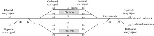
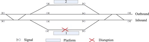
In a major disruption, trains in both directions (inbound and outbound) must be efficiently rescheduled. In the short-turning strategy, usually only the train services on one side of the disruption are considered, because the train-rescheduling problem is approximately symmetrical, e.g. see Louwerse and Huisman (2013) and Veelenturf et al. (2015). On a double-track high-speed railway line, inbound (outbound) train services normally use inbound (outbound) tracks in each segment. In the waiting strategy, if we assume that inbound (outbound) trains are only allowed to take inbound (outbound) sidings in each station, trains in both directions do not interrupt each other. Thus, trains in both directions can be rescheduled independently, and the two rescheduling tasks are performed separately; e.g. see Zhan et al. (2015). However, many Chinese high-speed railway stations for technical reasons allow trains in both directions to share the same station track. For example, in Humen Station on the Beijing-Hong Kong high-speed railway line (Figure 1), track 1 (the inbound maintrack) is typically used by trains running from left to right, and track 2 (the outbound maintrack) is typically used by trains running in the opposite direction. Maintracks are not equipped with platforms at most stations that are passed by such trains, such as Humen Station. Tracks 3, 4, 5 and 6 are station tracks equipped with platforms, called sidings, which can be used by dwell trains to board and alight passengers. Usually, tracks 3 and 4 are used by inbound trains and are denoted inbound sidings, and tracks 5 and 6 are used by outbound trains and are denoted outbound sidings. It is possible that trains in both directions can be allowed to share sidings in a station if they arrive at the corresponding siding via crossings in case of a complete blockage, which is helpful for reducing delays. For example, as shown in Figure 1, during a disruption inbound trains can arrive at siding 5 or 6 by crossing (2) on the left, and depart from these two sidings by using crossing (3) on the right. Accordingly, in this research we allow trains in both directions to share sidings in a station. Thus, train services in both directions are required to be rescheduled simultaneously because they will otherwise interrupt each other while passing through a station. For example, in a complete blockage, trains in both directions may interrupt each other by sharing the same siding after the disruption ends.

Figure 1. The layout of Humen Station on the Beijing-Hong Kong high-speed railway line.

We can imagine that rescheduling trains for each direction separately is simpler (fewer trains need to be handled at a time), but only a given part of sidings can be used for trains in each direction, so that the total delay of trains tends to be longer. However, if we simultaneously reschedule trains in both directions, all the available sidings in a station can be used by trains in each direction, and thus the total train delay can be further reduced.

1.1. Relevant studies

Train rescheduling in either a disturbance or a disruption has been a hot topic of research during the past decade. As defined by Cacchiani et al. (2014), ‘disturbance’ refers to small perturbations, while ‘disruption’ refers to relatively large incidents. This study, and hence the following literature review, focuses on train rescheduling in a disruption. We refer interested readers to surveys by Cacchiani et al. (2014), Corman and Meng (2015) and Fang, Yang, and Yao (2015) on train rescheduling in a disturbance. In addition, related research topics, first train and last train timetabling of a metro system can be found in Kang et al. (2016, 2015a); Kang and Meng (2017); Kang et al. (2019) and last train rescheduling of a metro system can be found in Kang et al. (2015b).

Train rescheduling in a disruption can be performed at both macroscopic and microscopic levels (Cacchiani et al. 2014). Macroscopic train rescheduling involves a high-level representation of railway infrastructure, such as stations and the segments between them. This keeps the problem relatively small-scale, allowing it to be solved in a shorter computational time, as per the requirements of real-time application. However, macroscopic solutions require the more detailed feasibility checking of station capacities.

(1) Macroscopic approaches for train rescheduling Brucker, Heitmann, and Knust (2002) rescheduled trains in a situation where one track of a double-track segment was unavailable because of construction activities. Assuming that the sequence of trains in each direction running outside the construction segment was fixed, these researchers devised the sequence of trains in both directions passing the construction segment to minimize the total train delay. However, they only considered train rescheduling during the construction period and did not examine how to subsequently recover a normal train service. Meng and Zhou (2011) also investigated the appropriate train orderings (i.e. train meeting and passage plans) in a disruption on a single-track railway line, handling the uncertainty in the duration of disruption using a scenario-based rolling horizon approach. However, the station capacity was not taken into account in their model. Albrecht, Panton, and Lee (2013) focused on train rescheduling in a disrupted situation where track maintenance was organized at a macroscopic level, in which both train operations and track maintenance were considered by regarding each track maintenance task as a pseudo train. A problem-space meta-heuristic search method was applied to ensure the rapid solution of the model to minimize the total delay for trains and maintenance.

Event-activity networks are widely applied in macroscopic train rescheduling. Louwerse and Huisman (2013) rescheduled trains in both partial and complete segment blockage based on an event-activity network. An ILP model was formulated to minimize the number of canceled trains and the total train delay. Veelenturf et al. (2015) extended the model of Louwerse and Huisman (2013) by considering the capacity of each station and the rolling stock circulation. Unlike Louwerse and Huisman (2013), they took into account the transfer from both the original timetable to the disposition timetable at the beginning of the disruption, and from the disposition timetable back to the original timetable at the end of the disruption. In Louwerse and Huisman (2013) and Veelenturf et al. (2015), trains were only allowed to short-turn at the last station adjacent to the disruption location. To increase the flexibility of train short-turning, Ghaemi, Cats, and Goverde (2018) developed a mixed integer linear programming (MILP) model to determine how to short-turn trains at multiple stations near the disruption location in a complete blockage. Zhu and Goverde (2019) further extended the flexibility of short-turning by allowing it to occur at every possible station. Van Aken, Bešinović, and Goverde (2017) introduced a train timetable adjustment model to reschedule trains where some tracks were unavailable due to station or open-track section maintenance. Their model was based on an extended periodic event scheduling problem (PESP), and train short-turning was determined in a preprocessing step.

In contrast, Zhan et al. (2015) rescheduled trains on a double-track high-speed railway line with a seat reservation system in a complete blockage. Short-turning was not allowed, and trains instead had to stop and wait for the end of a disruption. An MILP model was formulated to determine both the stop location and the departure and arrival times of trains based on an event-activity network. In the model, they assumed that inbound trains could only use inbound station tracks and outbound trains could only use outbound station tracks. Therefore, trains in opposite directions did not interrupt each other and could be rescheduled separately. Zhan et al. (2019) further determined the train stopping plan for trains in both directions of a high-speed railway line in a complete blockage. The interaction among trains in both directions was considered at a macroscopic level, but only trains scheduled to pass the disrupted segment were considered. Zhan et al. (2016) compared strategies for high-speed train rescheduling in a partial segment blockage, but as they considered both the inbound and outbound trains, the event-activity-based MILP model was difficult to solve. Thus, a rolling horizon approach was applied to decompose the model. Train scheduling under railway maintenance is a related research topic to our train rescheduling in a major disruption. Vansteenwegen et al. (2016) introduced a robust train timetable rescheduling approach to reduce the impact of infrastructure maintenance on the passenger service quality. In their model, train routing, timing and cancelation were considered.

(2) Microscopic approaches for train rescheduling

Microscopic train rescheduling is an alternative approach that uses a very precise representation of the railway infrastructure, i.e. at the track-circuit level, where the blocking-time model described by Hansen (2008) is used to calculate the track capacity. The solutions obtained by microscopic models are more practical for real-world applications. However, the problem size is usually large because more detailed information is considered, resulting in a long computational time for real-world problems. Corman et al. (2011) and Corman and D'Ariano (2012) rescheduled trains in a disrupted situation at a microscopic level, where one track of a segment was temporarily unavailable. They considered a network that was divided into several dispatching areas. In experiments, they assessed the solutions obtained by centralized dispatching and distributed dispatching strategies, showing that both solutions faced increasing difficulty in finding feasible schedules in a short computational time, as the time horizon was extended. Based on the microscopic train scheduling model in Pellegrini, Marlière, and Rodriguez (2014), Ghaemi, Cats, and Goverde (2017) developed an MILP model to solve the train short-turning problem in a complete blockage at a microscopic level. They tested their model on a short Dutch railway corridor considering only trains on one side of the blockage, showing that a disruption lasting up to one hour could be solved in a short computational time. However, efficient algorithms were necessary to solve larger cases. Hirai et al. (2009) investigated stopping patterns for trains at appropriate stations in a disrupted situation at a microscopic level, where the line was blocked by an accident for a long time. An integer programming model based on a Petri-net was formulated to solve the problem of train stopping deployment planning. However, a large number of parameters were required in the model, meaning that the model could become large and was not able to solve large real-world problems. Thus, due to the complexity of microscopic train rescheduling in large disruptions, microscopic models are mostly restricted to solving on-line train rescheduling in small perturbations, as done by Xu et al. (2017), or off-line train scheduling Pellegrini, Marlière, and Rodriguez (2014); Luan et al. (2017); D'Ariano et al. (2019); Zhang et al. (2019a).

(3) Mesoscopic approaches for train rescheduling

Considering that macroscopic and microscopic train rescheduling in a large disruption each has advantages and disadvantages, some researchers have tried to combine these two approaches: this attempt at combination is denoted the micro/macro principle. Dollevoet et al. (2014) introduced an iterative approach to solve a macroscopic delay management model on the one hand, and a microscopic train scheduling model on the other hand. The former approach helped to reduce the computational complexity, while the microscopic scheduling model at the station level enabled checking of the feasibility of the solution obtained by the macroscopic model. Similarly, Lamorgese, Mannino, and Piacentini (2016) solved the train dispatching problem by a Benders'-like decomposition algorithm, where macroscopic train rescheduling on the line was regarded as the master problem, and the microscopic train routing in a station was the slave problem. By iteratively solving the master and slave problems, an exact solution could be obtained for short- and middle-distance lines without complex rail nodes. However, as the train routing in a station is NP-complete Kroon, Edwin Romeijn, and Zwaneveld (1997) on its own, the slave problem is complicated for large stations. Wüst et al. (2019) focused on the maintenance timetable planning problem, which is done off-line. They extended the PESP and considered the railway infrastructure from a mesoscopic level.

(4) Decomposition solution approaches for train rescheduling

Most of the above-mentioned studies solved their train-rescheduling problem model using commercial solvers, e.g. CPLEX or Gurobi (Louwerse and Huisman 2013; Veelenturf et al. 2015; Ghaemi, Cats, and Goverde 2017, 2018; Zhu and Goverde 2019; Zhan et al. 2015; Corman et al. 2011; Xu et al. 2017). As train rescheduling in a large disruption is NP-hard, however, commercial solvers can struggle with large-scale problems. Therefore, a decomposition approach is often applied to divide the whole problem into several easy-to-solve subproblems. One approach is to decompose the whole problem in the time dimension, e.g. the rolling horizon approach used in Meng and Zhou (2011) and Zhan et al. (2016). In this instance, although solving a rescheduling problem via multiple short time horizons can reduce the complexity of the problem, the solution quality is sensitive to the length of the divided horizons. Another approach is to divide the whole problem in the spatial dimension, i.e. each subproblem corresponds to a local region. Here, by appropriately coordinating the local-region rescheduling problems, the whole problem is solved; this approach has been used by, for example, Corman et al. (2011) and Lamorgese, Mannino, and Piacentini (2016). A third approach is to combine the previous two approaches, i.e. decompose the whole problem in both space and time dimensions. This strategy was used in Meng and Zhou (2011, 2014) who also utilized Lagrangian relaxation (LR) for the decomposition. Although each single-train scheduling problem for the Lagrangian dual problem is easy to solve, the final solution of the dual problem is usually inapplicable to the primal problem. The optimality gap between the upper bound and lower bound can be large, e.g. more than 30% in Meng and Zhou (2014). To improve the primal feasibility of Lagrangian relaxation, the alternating direction method of multipliers (ADMM) has recently been applied in Yao et al. (2019) for the vehicle-routing problem, and in Zhang et al. (2019b) for the train-timetabling problem. Compared with Lagrangian relaxation, ADMM improves both the primal and dual feasibility, thus reducing the optimality gap and also the required number of iterations. For detailed information about the ADMM algorithm, we refer the reader to Boyd et al. (2011).

1.2. Objectives and contributions

We reschedule trains in both directions of a double-track railway network simultaneously by allowing inbound trains and outbound trains to share the same siding. A space-time network is constructed from a ‘mesoscopic’-level (i.e. a level intermediate between micro and macro) to describe our problem, and an ILP model is formulated based on the space-time network to solve the problem. Due to the complexity of the problem and the requirement of real-time applications, ADMM is used to decompose and solve the model. We also solve the model by LR to obtain the lower-bound solution, to evaluate the quality of the ADMM algorithm in solving the train-rescheduling problem. A real-world high-speed railway network, the Jinan-Nanjing line and the Bengbu-Hefei line in China, is used to test our model. In the case study, we compare the solution obtained by rescheduling trains in inbound and outbound directions simultaneously, where trains in both directions are allowed to share sidings (e.g. Corman et al. 2011 and Corman and D'Ariano 2012) with that obtained by rescheduling trains in each direction separately, where trains in both directions are prevented from sharing the same siding. To the best of our knowledge, our study is the first attempt to reschedule trains with simultaneous rerouting using a mesoscopic model for a large high-speed railway network and a long-time horizon. The aim is to rapidly obtain a good, feasible disposition timetable to assist dispatchers to quickly reschedule trains during a large disruption.

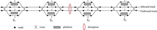
We make two main contributions to the field in this paper. First, we develop an ILP model to reschedule both inbound and outbound trains simultaneously, at a mesoscopic level, during a large disruption. Here, we make use of the fact that in many high-speed railway stations, trains traveling in either direction can share sidings during a serious disruption. To this end, our simultaneous rerouting approach outperforms the one-direction rerouting approach from a practical point of view. Second, we decompose the train-rescheduling problem into a series of easy-to-solve subproblems. The ADMM is applied to efficiently solve the ILP model, which has a sufficiently short computation time to solve train rescheduling for large networks with a long-time horizon by a mesoscopic model. The physical node in this study refers to the main signal point in a station area, e.g. the entry or exit signal within a station, see in Figure 2. The physical link is the track between two consecutive physical nodes.

Figure 2. A simple example of a double-track railway line.

The remainder of this paper is organized as follows. In Section 2, we describe the problem. An ILP model is formulated to model the high-speed train-rescheduling problem in a large disruption in Section 3. Section 4 introduces the ADMM and LR algorithms to solve the model. Section 5 presents the computational results. Conclusions and future research directions are discussed in Section 6.

2. Problem description

We focus on high-speed train rescheduling on a double-track railway network in a situation of a complete blockage. An example of a railway line consisting of four stations is shown in Figure 2. The railway line is denoted by a node-arc graph, as used in many previous studies (e.g. Caprara, Fischetti, and Toth 2002). However, the stations are not regarded as single nodes as in macroscopic rescheduling; instead, each station with four tracks is denoted by 12 nodes (see Figure 2), which helps one to model the detailed movements of a train within a station, such as passing, planned dwelling and extra stopping. However, unlike Pellegrini, Marlière, and Rodriguez (2014), we do not go into further detail to consider the route-lock sectional-release interlocking system at the track-circuit level, as this would be computationally expensive. We will explain various types of arcs in detail in Section 3. As mentioned previously, we allow inbound and outbound trains to share the same siding if it connects with both the inbound and outbound main tracks (a situation we denote as ‘technically possible’).

In a segment, the inbound main track is used by inbound trains, while the outbound main track is taken by outbound trains.

In the situation of the complete blockage of a segment during a disruption, trains cannot pass that segment. Thus, the dispatchers must reschedule trains based on their locations (on the original timetable) when a disruption occurs to minimize the deviation from the original timetable. Specifically, the dispatchers need to determine the departure and arrival time of each train at each station, the specific track that each train uses at each station that it visits, and whether some trains need to be canceled due to limited railway capacity, considering that the minimum running time in a segment and dwell time at a station for each train should be ensured and that conflicts between any two trains occupying incompatible track resources must be prevented. This study aims to assist dispatchers to make these decisions by providing them with a good disposition timetable.

In addition, we compare two rescheduling strategies in a disruption: rescheduling trains in both directions simultaneously by allowing trains in both directions to share sidings in a station and rescheduling trains in each direction separately by forbidding trains in both directions from sharing sidings in a station. Our solutions will assist railway managers or dispatchers to optimize their rescheduling strategies.

3. Model formulation

In this section, we first make some assumptions and define the notation that will be used in our model. Then we introduce a space-time network at a meso-level to describe our train-rescheduling problem. Finally, we develop an ILP model based on the space-time network.

3.1. Assumptions and notations

In our model, the following assumptions are made:

•	Inbound trains and outbound trains can share the same siding, if this is technically possible. However, a track of a segment can only be used by trains running in the same direction.
•	Trains that have entered the disrupted segment when a disruption occurs can continue.
•	Before the disruption occurs, all train services operate according to the original timetable.
•	The duration of a disruption is known in advance.
•	We reschedule trains in a given time window which is longer than the duration of the disruption, and train rescheduling in other time periods can be done in a similar manner.

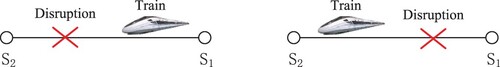
The first assumption is based on the practical fact that each siding in many high-speed railway stations is connected with both maintracks by crossings. Therefore, this assumption is technically reasonable. The second assumption implies that trains have already passed the disrupted location if they entered the disrupted section before the disruption occurs; see the right subgraph in Figure 3 where the train runs from station $S_1$ to $S_2$ on section $(S_1,S_2)$. If we know of a specific train that entered the disrupted section (i.e. a link between two stations when a segment is blocked or a station track when a track of a station is blocked) but did not pass the disrupted location before the disruption occurred (see the left subgraph in Figure 3), we can let it return to stop at the nearest station ($S_1$), which is easy to handle by slightly revising the input of our model. According to the practice of Chinese railway, if a train stops at a segment due to a disruption, it is allowed to go back to the nearest station to clear the segment track for rescue trains. We make the third assumption because trains normally run as scheduled on a high-speed railway line. The last assumption is comparatively strong, although it has been made in most previous studies. Handling the uncertainty of a disruption is a difficult topic, and is not the focus of this research. Interested readers are referred to Meng and Zhou (2011), Zhan et al. (2016), and Zilko, Kurowicka, and Goverde (2016) for more information about how to handle the uncertainty in the duration of a disruption. However, we will reschedule trains under various disruptions with different durations.

Figure 3. An example for a train passes a disrupted location in a segment between two stations.

Our meso-level train-rescheduling model is formulated based on a space-time network. The basic notation used in the model formulation is introduced in Table 1.

Table 1. Notation used in the space-time network-based model.

Notation	Description
Sets:
T	Set of times, $t,t^{\prime },\tau ,{\tau }^{\prime }\in T$
N	Set of physical nodes, $i,i^{\prime },j,j^{\prime }\in N$
$N^k\subset N$	Set of physical nodes available for train k
$S_k$	Set of stations visited by train k.
L	Set of physical links connecting two neighboring physical nodes, $(i,j)\in L$
K	Set of train services, $k\in K$
E	Set of time-expanded nodes, $(i,t)\in E$
$E^k\subset E$	Set of time-expanded nodes available for train k, $(i,t)\in E^k$
A	Set of time-expanded arcs, $(i,j,t,t^{\prime })\in A$
$A^k\subset A$	Set of time-expanded arcs available for train k
$\tilde{A}$	Set of time-expanded virtual arcs, $(i,j,t,t^{\prime })\in \tilde{A}$
$A_i^{k,+}\subset A^k$	Set of available arcs of train $k\in K$ leaving node $i\in N^k$
$A_i^{k,-}\subset A^k$	Set of available arcs of train $k\in K$ entering node $i\in N^k$
$A_k^s$	Set of possible arrival arcs of train k at station s
${\mathrm{\Omega }}_{(i,t)}\subset E$	Set of departure (arrival) nodes incompatible with node $(i,t)$
${\mathrm{\Omega }}_{(i,j,t,t^{\prime })}^{\prime }\subset A$	Set of conflicting arcs with arc $(i,j,t,t^{\prime })$ corresponding to a station path
Parameters:
$\hat{T}$	End time of the planned time horizon
$c_{i,j,t,t^{\prime }}^k$	Train operation cost on arc $(i,j,t,t^{\prime })\in A$ for train k
$C_k^0$	The cancelation cost of train k
$o_k$	Origin of train k
$d_k$	Destination of train k
$e_k$	Earliest departure time of train k from its origin
$l_k$	Latest arrival time of train k at its destination
$t_{k,s}^o$	Planned arrival time of train k at station s
$H_{dis}^{start}$	Start time of disruption
$H_{dis}^{end}$	End time of disruption
$h_{dep}^{min}$	Minimum departure headway of two trains in a segment
$h_{arr}^{min}$	Minimum arrival headway of two trains in a segment
$h_{station}^{min}$	Minimum headway of two trains using the same station path
Decision variable:
$x_{i,j,t,t^{\prime }}^k$	A binary variable, if train k uses arc $(i,j,t,t^{\prime })$, $x_{i,j,t,t^{\prime }}^k=1$; otherwise, $x_{i,j,t,t^{\prime }}^k=0$.

3.2. Space-time network

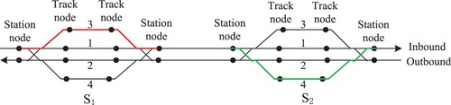
To illustrate the space-time network, we first show a small physical railway line consisting of two stations with one segment between them; see Figure 4. As mentioned in the problem description, each station has four tracks and is denoted by 12 nodes. A node is a main signal point of a station, i.e. the entry and exit points of a station (station nodes) and the end points of each station track (track nodes), see in Figure 4. A station path that is used by a train to pass a station with or without dwelling starts from a station node and ends at another station node at the other side of the station. For example, one of the possible paths for a train that passes station $S_1$ in the direction from $S_1$ to station $S_2$ is shown by a red line, and is a ‘normal’ path (i.e. it involves an inbound train using an inbound siding, such as 3). As we allow trains in both directions to use any possible siding in a station during a disruption if the siding is connected with the used maintrack, a train running from $S_1$ to $S_2$, can use the path shown by the green line to pass $S_2$, which is an ‘unusual’ path (i.e. it involves an inbound train using an outbound siding, such as 4).

Figure 4. A simple physical railway line.

In a space-time network, time is discretized into n time intervals, and a time horizon $T=\{0,\delta ,2\delta ,\dots ,n\delta \}$. The length of time interval δ is determined as required, e.g. 1 min or 30  s. In this research, we choose 1 min as the length of the time interval. We extend the physical railway network $\overline{G}=(N,L)$ to a space-time network by adding a time dimension, $G=(E,A)$, where E is the set of time-expanded nodes corresponding to physical nodes set N, and A is the set of time-expanded arcs corresponding to physical link set L. A time-expanded arc $(i,j,t,t^{\prime })\in A$, connecting two time-expanded nodes $(i,t)\in E$ and $(j,t^{\prime })\in E$, denotes that a train starts from node i at time t and ends at node j at time $t^{\prime }$.

Each train ($k\in K$) runs from its origin node $o_k$ to its destination node $d_k$. We assume that the earliest start time from its origin and the latest arrival time at its destination are $e_k$ and $l_k$, respectively. It is possible that some trains may not operate at all because of the limited railway capacity in a disruption. Therefore, an artificial arc is introduced to denote the path of a canceled train, in which the arc starts from the train's origin at time $e_k$ and ends at its destination at time $l_k$. We denote the artificial train arc set of all canceled trains as $\tilde{A}$. Hence, the artificial arc for a train k is $(o_k,d_k,e_k,l_k)$, $(o_k,d_k,e_k,l_k)\in \tilde{A}$.

In our space-time network, the following types of arcs are defined to represent the movement of a train from its origin to its destination. We use a train k running from station $S_1$ to station $S_2$ on a physical railway line in Figure 4 as an example to explain all of the possible types of train arc. To better distinguish different types of arcs, we define space-time node subset $E^{SN}\subset E$ including all nodes $(i,t)$ where i is a station node in Figure 4; and we also define a node subset $E^{TN}\subset E$ including all nodes $(i,t)$ where i is a track node in Figure 4. A simple example is given in Figure 5 to clarify the meaning of each type of arc.

•	Origin-wait arc: an origin-wait arc is a unit arc, denoting that a train waits at its origin for 1 min due to having a late departure. The origin-wait arc set is $A^{owait}=\{(o_k,o_k,t,t+\delta )|(o_k,t),(o_k,t+\delta )\in E\}$. If a train waits at its origin for several min, several successive origin-wait arcs are used to denote the waiting process.
•	Access arc: an access arc represents a train starting from its origin (e.g. the shunting yard) and traveling to the station node of the first station in the transportation system. The set of arcs of this kind is denoted as $A^{access}=\{(o_k,j,t,t^{\prime })|(o_k,t)\in E,(j,t^{\prime })\in E^{SN}\}$. Here j is the left station node in station $S_1$ on the inbound maintrack in Figure 4.
•	Enter arc: an enter arc represents a movement of a train from a station node to a neighboring track node of an available track in the same station. The set of enter arcs is expressed as $A^{enter}=\{(i,j,t,t^{\prime })|(i,t)\in E^{SN},(j,t^{\prime })\in E^{TN}\}$. For example, i is the left station node of station $S_1$ on the inbound maintrack, and j is the left track node of a station track in $S_1$ in Figure 4.
•	Pass arc: a pass arc represents a train passing a station without stopping to allow passengers to board and alight. A pass arc connects one track node $(i,t)$ of a station track with the other track node $(j,t^{\prime })$ of the same station track. The set of arcs of this kind can be expressed as $A^{pass}=\{(i,j,t,t^{\prime })|(i,t)\in E^{TN},(j,t^{\prime })\in E^{TN},(t^{\prime }-t)=TP(i,j)\}$. Here, $TP(i,j)$ is the time that a train passes a station without a scheduled stop.
•	Dwell arc: a dwell arc represents a train waiting at a station to board and alight passengers. A dwell arc connects one track node $(i,t)$ of a station track to the other track node $(j,t^{\prime })$ of the same station track. The set of arcs of this kind can be expressed as $A^{dwell}=\{(i,j,t,t^{\prime })|(i,t)\in E^{TN},(j,t^{\prime })\in E^{TN},(t^{\prime }-t)=TW(i,j)\}$, where i and j are the two track nodes of a station track. $TW(i,j)$ is the time that a train passes a station with a scheduled stop.
•	Extra-wait arc: an extra-wait arc represents a train waiting on a station track for a longer time than the scheduled time, and is a unit arc. If the extra waiting time of a train is longer than δ min, it is represented by several successive extra-wait arcs. The set of arcs of this kind is expressed as $A^{ewait}=\{(i,i,t,t+\delta )|(i,t),(i,t+\delta )\in E^{TN}\}$, where node i is a track node (the right track node of a track) in Figure 4.
•	Exit arc: an exit arc represents a train leaving a station track from the track node to the following station node. An exit arc starts at a track node of a station track, $(i,t)$, and ends at a station node of the same station, $(j,t^{\prime })$. The set of arcs of this kind is defined as $A^{exit}=\{(i,j,t,t^{\prime })|(i,t)\in E^{TN},(j,t^{\prime })\in E^{SN}\}$.
•	Drive arc: a drive arc represents a train running in a segment between two stations. It connects a station node of one station, $(i,t)$, to a station node of the following station of the same maintrack, $(j,t^{\prime })$. The set of arcs of this kind is $A^{drive}=\{(i,j,t,t^{\prime })|(i,t)\in E^{SN},(j,t^{\prime })\in E^{SN}\}$. For instance, i is the right station node of station $S_1$, and j is the left station node of station $S_2$ on the inbound maintrack in Figure 4.
•	Egress arc: an egress arc represents a train leaving the last station for its destination (e.g. a shunting yard). This arc set is expressed as: $A^{egress}=\{(i,d_k,t,t^{\prime })|(i,t)\in E^{SN},(d_k,t^{\prime })\in E\}$, where $(i,t)$ is the last station node of the last station and $(d_k,t^{\prime })$ is the node corresponding to the train's destination.
•	Destination-hold arc: a destination-hold arc is a unit arc, that represents a train finally stopping at the shunting yard. This arc set is $A^{dhold}=\{(d_k,d_k,t,t+\delta )|(d_k,t),(d_k,t+\delta )\in E\}$. We use arcs of this kind to denote a train k stopping at its shunting yard at its final arrival time $l_k$.
•	Artificial arc: an artificial arc represents a train starting from its origin at the earliest departure time and arriving at its destination at the latest arrival time. This arc set can be denoted as: $\tilde{A}=\{(o_k,d_k,e_k,l_k)|\mathrm{\forall }k\in K\}$.

Figure 5. A simple space-time network for a train.

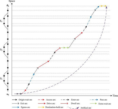
According to the definitions of the various types of arcs, the set consisting of all of the space-time arcs is denoted as $A=A^{owait}\cup A^{access}\cup A^{enter}\cup A^{dwell}\cup A^{pass}\cup A^{ewait}\cup A^{exit}\cup A^{drive}\cup A^{egress}\cup A^{dhold}\cup \tilde{A}$. As mentioned previously, our meso-level train-rescheduling model considers trains passing stations in more detail than the macro-level models. Specifically, we have an enter arc and an exit arc to denote a train entering a station and leaving a station through the throat area of a station, a pass arc to denote a train passing a station without a stop, a dwell arc to model a train having a planned stop, and an extra-wait arc to represent a longer stop time than the planned time due to a disruption. Note that the definitions of dwell arc and pass arc are similar, but the process time of them is different. The aim to distinguish these two arcs is to model the required dwell time of a train at a station. The minimum dwell time of a train at a station is ensured by a dwell arc. A simple example of one train and three stations (each having two tracks) is shown in Figure 5 to illustrate the purpose of the various space-time arcs. In this figure, we can see that a train departs from its origin $o_k$ and finally arrives at its destination $d_k$ by using various types of space-time arcs (denoted by different allow lines or colors) defined previously. In case a train uses an artificial arc, it is canceled.

3.3. Model based on space-time network

In most of the existing research, the train scheduling and rescheduling problem was formulated by an ILP or MILP model with many big ‘M’ constraints (e.g. Meng and Zhou 2014; Veelenturf et al. 2015; Zhan et al. 2015). However, these kinds of models tend to produce weak relaxations and consequently large search trees. To strengthen the formulation, we build our model based on a space-time network, which is known to help to eliminate the common big ‘M’ constraints. The space-time network has previously been applied in train-scheduling and -rescheduling problems; see Zhou and Teng (2016) and Meng and Zhou (2014) for instance. Note that our space-time network is different from those used in Kliewer, Mellouli, and Suhl (2006), Steinzen et al. (2010) and Olsen, Kliewer, and Wolbeck (2020), in which space-time networks are used to reduce the deadheading arcs in multiple-depot bus scheduling. Our meso model is partly similar to that in Kecman et al. (2013) where train rescheduling is considered in detail, close to a microscopic level.

To formulate the train-rescheduling model, we first define an incompatible arc set ${\mathrm{\Omega }}_{(i,j,t,t^{\prime })}$ to model the departure and arrival headway constraints between two trains, similar to the method found, for example, in Caprara, Fischetti, and Toth (2002) for railway timetabling. For a space-time drive arc $(i,j,t,t^{\prime })\in A^{drive}$, its incompatible arc set ${\mathrm{\Omega }}_{(i,j,t,t^{\prime })}$ is defined as follows (Equation (1(1) ${\mathrm{\Omega }}_{(i,j,t,t^{\prime })}=\{(i,j,\tau ,{\tau }^{\prime }):|t-\tau |<h_{dep}^{min}\cup |t^{\prime }-{\tau }^{\prime }|<h_{arr}^{min}\cup (t-\tau )\times (t^{\prime }-{\tau }^{\prime })<0\}$(1) )): (1) ${\mathrm{\Omega }}_{(i,j,t,t^{\prime })}=\{(i,j,\tau ,{\tau }^{\prime }):|t-\tau |<h_{dep}^{min}\cup |t^{\prime }-{\tau }^{\prime }|<h_{arr}^{min}\cup (t-\tau )\times (t^{\prime }-{\tau }^{\prime })<0\}$(1) where parameters $h_{dep}^{min}$ and $h_{arr}^{min}$ are the minimum departure and arrival headway time between two trains, respectively. The overtaking between two trains in a segment is prevented by $(t-\tau )\times (t^{\prime }-{\tau }^{\prime })<0$, which denotes that the order of the two trains does not change in a segment. Equation (1(1) ${\mathrm{\Omega }}_{(i,j,t,t^{\prime })}=\{(i,j,\tau ,{\tau }^{\prime }):|t-\tau |<h_{dep}^{min}\cup |t^{\prime }-{\tau }^{\prime }|<h_{arr}^{min}\cup (t-\tau )\times (t^{\prime }-{\tau }^{\prime })<0\}$(1) ) denotes that if an arc $(i,j,t,t^{\prime })\in A^{drive}$ is used by a train, any other arc $(i,j,\tau ,{\tau }^{\prime })\in A^{drive}$ with a smaller departure or arrival headway than the minimum value between $(i,j,t,t^{\prime })$ belongs to the incompatible arc set ${\mathrm{\Omega }}_{(i,j,t,t^{\prime })}$, which cannot be used by any other train. Similar modeling methods have been used in some previous studies, e.g. Caimi et al. (2009).

As discussed by Caprara, Fischetti, and Toth (2002), it is better to formulate the headway constraint by nodes instead of links. Thus, we further model the headway by nodes corresponding to trains' departure and arrival. According to Jiang, Cacchiani, and Toth (2017), it is complicated to model the headway constraint by departure nodes when trains have different running times in a segment. Therefore, we model the headway by both departure nodes (departure headway) and arrival nodes (arrival headway). Because the minimum departure headway and arrival headway are both 3 min and the running time difference for a high-speed train and a medium-speed train in any segment is smaller than 6 min in our case study, overtaking between two trains when they meet the departure headway and arrival headway in the end nodes of a segment can never happen. As a result, we can omit the overtaking constraint in this study. The departure headway constraint can be formulated by the incompatible node set of a departure node $(i,t)$ by Equation (2(2) ${\mathrm{\Omega }}_{(i,t)}=\{(i,t^{\prime }):|t^{\prime }-t|<h_{dep}^{min}\}$(2) ). Here departure node is the station node entering the following segment, i.e. the right station node of $S_1$ in Figure 4 for inbound trains. (2) ${\mathrm{\Omega }}_{(i,t)}=\{(i,t^{\prime }):|t^{\prime }-t|<h_{dep}^{min}\}$(2) The arrival headway constraint can be formulated by the incompatible node set of an arrival node $(i,t)$ by Equation (3(3) ${\mathrm{\Omega }}_{(i,t)}=\{(i,t^{\prime }):|t^{\prime }-t|<h_{arr}^{min}\}$(3) ). Here arrival node is the station node exiting the previous segment, i.e. the left station node of $S_s$ in Figure 4 for inbound trains. (3) ${\mathrm{\Omega }}_{(i,t)}=\{(i,t^{\prime }):|t^{\prime }-t|<h_{arr}^{min}\}$(3) Similarly, we also define an incompatible arc set to model the station capacity constraint. From our space-time network for trains constructed above, we can see that five types of arcs can possibly correspond to a station path, $(i,j,t,t^{\prime })\in A^{enter}$, $(i,j,t,t^{\prime })\in A^{pass}$, $(i,j,t,t^{\prime })\in A^{dwell}$, $(i,j,t,t^{\prime })\in A^{ewait}$, and $(i,j,t,t^{\prime })\in A^{exit}$. Here, a station path means the route taken by a train in passing through a station. As each station path (e.g. the path shown by the red or green lines in Figure 4) can be used by at most one train at a certain time in a route-lock route-release interlocking system, all of the arcs corresponding to a station path can be simultaneously occupied by only one train. That is, they are incompatible among different trains either in the same direction or in the opposite direction. For each arc $(i,j,t,t^{\prime })\in A^{enter}\cup A^{pass}\cup A^{dwell}\cup A^{ewait}\cup A^{exit}$ corresponding to a station path, its incompatible arc set ${\mathrm{\Omega }}_{(i,j,t,t^{\prime })}^{\prime }$ is defined as follows (Equation (4(4) ${\mathrm{\Omega }}_{(i,j,t,t^{\prime })}^{\prime }=\{(i^{\prime },j^{\prime },\tau ,{\tau }^{\prime }):(t-{\tau }^{\prime })<h_{station}^{min}\cup (\tau -t^{\prime })<h_{station}^{min}\}$(4) )): (4) ${\mathrm{\Omega }}_{(i,j,t,t^{\prime })}^{\prime }=\{(i^{\prime },j^{\prime },\tau ,{\tau }^{\prime }):(t-{\tau }^{\prime })<h_{station}^{min}\cup (\tau -t^{\prime })<h_{station}^{min}\}$(4) Equation (4(4) ${\mathrm{\Omega }}_{(i,j,t,t^{\prime })}^{\prime }=\{(i^{\prime },j^{\prime },\tau ,{\tau }^{\prime }):(t-{\tau }^{\prime })<h_{station}^{min}\cup (\tau -t^{\prime })<h_{station}^{min}\}$(4) ) indicates that if an arc $(i,j,t,t^{\prime })$ is occupied by a train, any other arc $(i^{\prime },j^{\prime },\tau ,{\tau }^{\prime })\in A^{enter}\cup A^{pass}\cup A^{dwell}\cup A^{ewait}\cup A^{exit}$ corresponding to the same station path as arc $(i,j,t,t^{\prime })$ with a headway less than $h_{station}^{min}$ min belongs to the incompatible arc set ${\mathrm{\Omega }}_{(i,j,t,t^{\prime })}^{\prime }$. Note that we allow trains in opposite directions to share sidings, and we therefore need to consider arcs that are used either by inbound trains or by outbound trains corresponding to the same station path in the incompatible arc set.

We minimize the total train arrival deviation which refers to the total arrival delay and arrival earliness of a train at each station it visits. That is, we do not consider the departure delay and earliness. Here the arrival time of a train at a station is the end time ($t^{\prime }$) of an enter arc $(i,j,t,t^{\prime })\in A^{enter}$. All of the possible enter arcs for a train in a station belong to arc set $A_k^s\subset A^{enter}$. The model is as follows (Objective (5(5) $\begin{array}{rlr}\mathbf{\text{min:}}& Z=\sum _{k\in K}\sum _{(i,j,t,t^{\prime })\in A_k}{c}_{i,j,t,t^{\prime }}^k\times x_{i,j,t,t^{\prime }}^k& \end{array}$(5) ) and Constraints (6(6) $\begin{array}{rl}\mathbf{\text{subject to:}}& \\ & \sum _{(i,j,t,t^{\prime })\in A_{o_k}^{k,+}}{x}_{i,j,t,t^{\prime }}^k=1\mathrm{\forall }k\in K\end{array}$(6) )–(12(12) $\begin{array}{rl}& x_{i,j,t,t^{\prime }}^k\in \{0,1\}\mathrm{\forall }(i,j,t,t^{\prime })\in A,\mathrm{\forall }k\in K\end{array}$(12) )): (5) $\begin{array}{rlr}\mathbf{\text{min:}}& Z=\sum _{k\in K}\sum _{(i,j,t,t^{\prime })\in A_k}{c}_{i,j,t,t^{\prime }}^k\times x_{i,j,t,t^{\prime }}^k& \end{array}$(5) (6) $\begin{array}{rl}\mathbf{\text{subject to:}}& \\ & \sum _{(i,j,t,t^{\prime })\in A_{o_k}^{k,+}}{x}_{i,j,t,t^{\prime }}^k=1\mathrm{\forall }k\in K\end{array}$(6) (7) $\begin{array}{rl}& \sum _{(i,j,t,t^{\prime })\in A_i^{k,-}}{x}_{i,j,t,t^{\prime }}^k=\sum _{(j,i,t,t^{\prime })\in A_i^{k,+}}{x}_{j,i,t,t^{\prime }}^k\mathrm{\forall }k\in K,\mathrm{\forall }i\in N^k:i\ne o_k\cap i\ne d_k\end{array}$(7) (8) $\begin{array}{rl}& \sum _{(i,j,t,t^{\prime })\in A_{d_k}^{k,-}}{x}_{i,j,t,t^{\prime }}^k=1\mathrm{\forall }k\in K\end{array}$(8) (9) $\begin{array}{rl}& \sum _{k\in K}\sum _{(i,t^{\prime })\in \mathrm{\Omega }(i,t):(i,j^{\prime },t^{\prime },{\tau }^{\prime })\in A^{drive}}{x}_{i,j^{\prime },t^{\prime },{\tau }^{\prime }}^k\le 1\mathrm{\forall }(i,t)\in E^{dep}\end{array}$(9) (10) $\begin{array}{rl}& \sum _{k\in K}\sum _{(i,t^{\prime })\in \mathrm{\Omega }(i,t):(j^{\prime },i,{\tau }^{\prime },t^{\prime })\in A^{drive}}{x}_{j^{\prime },i,{\tau }^{\prime },t^{\prime }}^k\le 1\mathrm{\forall }(i,t)\in E^{arr}\end{array}$(10) (11) $\begin{array}{rl}& \sum _{k\in K}\sum _{(i^{\prime },j^{\prime },\tau ,{\tau }^{\prime })\in {\mathrm{\Omega }}^{\prime }(i,j,t,t^{\prime })}{x}_{i^{\prime },j^{\prime },\tau ,{\tau }^{\prime }}^k\le 1\mathrm{\forall }(i,j,t,t^{\prime })\in A^{Spath}\end{array}$(11) (12) $\begin{array}{rl}& x_{i,j,t,t^{\prime }}^k\in \{0,1\}\mathrm{\forall }(i,j,t,t^{\prime })\in A,\mathrm{\forall }k\in K\end{array}$(12) In objective (5(5) $\begin{array}{rlr}\mathbf{\text{min:}}& Z=\sum _{k\in K}\sum _{(i,j,t,t^{\prime })\in A_k}{c}_{i,j,t,t^{\prime }}^k\times x_{i,j,t,t^{\prime }}^k& \end{array}$(5) ), we minimize the total train arrival deviation cost (arrival delay cost and arrival earlier cost) and train cancelation cost. Therefore, the cost coefficient $c_{i,j,t,t^{\prime }}^k$ can be defined by Equation (13(13) $c_{i,j,t,t^{\prime }}^k=\{\begin{array}{ll}{t}^{\prime }-t_{k,s}^o& \mathrm{\forall }(i,j,t,t^{\prime })\in A_k^s:t^{\prime }>t_{k,s}^o\\ t_{k,s}^o-t^{\prime }& \mathrm{\forall }(i,j,t,t^{\prime })\in A_k^s:t^{\prime }<t_{k,s}^o\\ C_k^0& \mathrm{\forall }(i,j,t,t^{\prime })\in \tilde{A}\\ 0& \text{otherwise}\end{array}$(13) ). (13) $c_{i,j,t,t^{\prime }}^k=\{\begin{array}{ll}{t}^{\prime }-t_{k,s}^o& \mathrm{\forall }(i,j,t,t^{\prime })\in A_k^s:t^{\prime }>t_{k,s}^o\\ t_{k,s}^o-t^{\prime }& \mathrm{\forall }(i,j,t,t^{\prime })\in A_k^s:t^{\prime }<t_{k,s}^o\\ C_k^0& \mathrm{\forall }(i,j,t,t^{\prime })\in \tilde{A}\\ 0& \text{otherwise}\end{array}$(13) Constraints (6(6) $\begin{array}{rl}\mathbf{\text{subject to:}}& \\ & \sum _{(i,j,t,t^{\prime })\in A_{o_k}^{k,+}}{x}_{i,j,t,t^{\prime }}^k=1\mathrm{\forall }k\in K\end{array}$(6) ), (7(7) $\begin{array}{rl}& \sum _{(i,j,t,t^{\prime })\in A_i^{k,-}}{x}_{i,j,t,t^{\prime }}^k=\sum _{(j,i,t,t^{\prime })\in A_i^{k,+}}{x}_{j,i,t,t^{\prime }}^k\mathrm{\forall }k\in K,\mathrm{\forall }i\in N^k:i\ne o_k\cap i\ne d_k\end{array}$(7) ) and (8(8) $\begin{array}{rl}& \sum _{(i,j,t,t^{\prime })\in A_{d_k}^{k,-}}{x}_{i,j,t,t^{\prime }}^k=1\mathrm{\forall }k\in K\end{array}$(8) ) are the train-flow conservation constraints. They ensure that each train can depart from its origin and finally arrive at its destination. Note that if a train is completely canceled, we assume that it uses an artificial arc to complete the journey and a relatively large penalty ($C_k^0$ in Equation (13(13) $c_{i,j,t,t^{\prime }}^k=\{\begin{array}{ll}{t}^{\prime }-t_{k,s}^o& \mathrm{\forall }(i,j,t,t^{\prime })\in A_k^s:t^{\prime }>t_{k,s}^o\\ t_{k,s}^o-t^{\prime }& \mathrm{\forall }(i,j,t,t^{\prime })\in A_k^s:t^{\prime }<t_{k,s}^o\\ C_k^0& \mathrm{\forall }(i,j,t,t^{\prime })\in \tilde{A}\\ 0& \text{otherwise}\end{array}$(13) )) is given to the arc cost $c_{ijtt}^k$. Partial cancelation is not allowed in this study. In these three flow conservation constraints, the available arcs for each train (arc sets $A_{o_k}^{k,+}$, $A_i^{k,-}$, $A_i^{k,+}$ and $A_{d_k}^{k,-}$) correspond to a specific train $k\in K$. Therefore, whether an arc can be used by a train is included, i.e. we only need to remove the arcs corresponding to a siding if the siding cannot be used by the train. Furthermore, if we only reschedule trains in one direction, the available arc sets ($A_{o_k}^{k,+}$, $A_i^{k,-}$, $A_i^{k,+}$ and $A_{d_k}^{k,-}$) for a train k correspond to part of the sidings. However, if we simultaneously reschedule trains in both directions, the available arc sets ($A_{o_k}^{k,+}$, $A_i^{k,-}$, $A_i^{k,+}$ and $A_{d_k}^{k,-}$) for a train k correspond to all the sidings. Constraints (9(9) $\begin{array}{rl}& \sum _{k\in K}\sum _{(i,t^{\prime })\in \mathrm{\Omega }(i,t):(i,j^{\prime },t^{\prime },{\tau }^{\prime })\in A^{drive}}{x}_{i,j^{\prime },t^{\prime },{\tau }^{\prime }}^k\le 1\mathrm{\forall }(i,t)\in E^{dep}\end{array}$(9) ) and (10(10) $\begin{array}{rl}& \sum _{k\in K}\sum _{(i,t^{\prime })\in \mathrm{\Omega }(i,t):(j^{\prime },i,{\tau }^{\prime },t^{\prime })\in A^{drive}}{x}_{j^{\prime },i,{\tau }^{\prime },t^{\prime }}^k\le 1\mathrm{\forall }(i,t)\in E^{arr}\end{array}$(10) ) are the departure headway constraint and arrival headway constraint, respectively, where set $E^{dep}$ consists of the station node entering a segment and set $E^{arr}$ consists of the station node exiting a segment, which has been explained and used in Equations (2(2) ${\mathrm{\Omega }}_{(i,t)}=\{(i,t^{\prime }):|t^{\prime }-t|<h_{dep}^{min}\}$(2) ) and (3(3) ${\mathrm{\Omega }}_{(i,t)}=\{(i,t^{\prime }):|t^{\prime }-t|<h_{arr}^{min}\}$(3) ). Constraint (11(11) $\begin{array}{rl}& \sum _{k\in K}\sum _{(i^{\prime },j^{\prime },\tau ,{\tau }^{\prime })\in {\mathrm{\Omega }}^{\prime }(i,j,t,t^{\prime })}{x}_{i^{\prime },j^{\prime },\tau ,{\tau }^{\prime }}^k\le 1\mathrm{\forall }(i,j,t,t^{\prime })\in A^{Spath}\end{array}$(11) ) is a station capacity constraint, which denotes that at most one train can use a path in a station at any time t. Constraint (12(12) $\begin{array}{rl}& x_{i,j,t,t^{\prime }}^k\in \{0,1\}\mathrm{\forall }(i,j,t,t^{\prime })\in A,\mathrm{\forall }k\in K\end{array}$(12) ) shows the domain of binary variable $x_{i,j,t,t^{\prime }}^k$. Note that, as we assume that trains run according to the original timetabling, we only need to reschedule trains after the disruption occurs.

4. Solution approaches

In this section, we first introduce the ADMM algorithm to decompose our model, with the aim of obtaining a good feasible solution in a short computational time (i.e. within several minutes). Then, we apply the LR algorithm to decompose the model to obtain lower-bound solutions, which can be used to evaluate the quality of the solution obtained by ADMM. Because ADMM is an extension of Augmented Lagrangian method, a quadratic penalty term is added in the objective function of the relaxed problem with a relatively large penalty parameter ρ. It is possible to obtain a solution for the relaxed problem which is feasible for the primal problem, but the obtained solution may not be a lower-bound solution or an optimal solution of the primal problem due to the added quadratic term. However, LR does not have a quadratic term compared with ADMM. It is usually applied to obtain a lower-bound solution that is usually infeasible for the primal problem.

4.1. Optimization framework based on ADMM

In the ILP model, most of the constraints correspond to a single train, with only Constraints (9(9) $\begin{array}{rl}& \sum _{k\in K}\sum _{(i,t^{\prime })\in \mathrm{\Omega }(i,t):(i,j^{\prime },t^{\prime },{\tau }^{\prime })\in A^{drive}}{x}_{i,j^{\prime },t^{\prime },{\tau }^{\prime }}^k\le 1\mathrm{\forall }(i,t)\in E^{dep}\end{array}$(9) ), (10(10) $\begin{array}{rl}& \sum _{k\in K}\sum _{(i,t^{\prime })\in \mathrm{\Omega }(i,t):(j^{\prime },i,{\tau }^{\prime },t^{\prime })\in A^{drive}}{x}_{j^{\prime },i,{\tau }^{\prime },t^{\prime }}^k\le 1\mathrm{\forall }(i,t)\in E^{arr}\end{array}$(10) ) and (11(11) $\begin{array}{rl}& \sum _{k\in K}\sum _{(i^{\prime },j^{\prime },\tau ,{\tau }^{\prime })\in {\mathrm{\Omega }}^{\prime }(i,j,t,t^{\prime })}{x}_{i^{\prime },j^{\prime },\tau ,{\tau }^{\prime }}^k\le 1\mathrm{\forall }(i,j,t,t^{\prime })\in A^{Spath}\end{array}$(11) ) corresponding to multiple trains. Therefore, we relax these constraints by ADMM to simplify the decomposition of the model. In principle, ADMM is applied to handle equality constraints. However, it is also can be applied to deal with inequality constraints by transferring inequality constraints to equality constraints. Therefore, in this study, we transfer Constraints (9(9) $\begin{array}{rl}& \sum _{k\in K}\sum _{(i,t^{\prime })\in \mathrm{\Omega }(i,t):(i,j^{\prime },t^{\prime },{\tau }^{\prime })\in A^{drive}}{x}_{i,j^{\prime },t^{\prime },{\tau }^{\prime }}^k\le 1\mathrm{\forall }(i,t)\in E^{dep}\end{array}$(9) )–(11(11) $\begin{array}{rl}& \sum _{k\in K}\sum _{(i^{\prime },j^{\prime },\tau ,{\tau }^{\prime })\in {\mathrm{\Omega }}^{\prime }(i,j,t,t^{\prime })}{x}_{i^{\prime },j^{\prime },\tau ,{\tau }^{\prime }}^k\le 1\mathrm{\forall }(i,j,t,t^{\prime })\in A^{Spath}\end{array}$(11) ) to equality constraints (14(14) $\begin{array}{rl}& \sum _{k\in K}\sum _{(i,t^{\prime })\in \mathrm{\Omega }(i,t):(i,j^{\prime },t^{\prime },{\tau }^{\prime })\in A^{drive}}{x}_{i,j^{\prime },t^{\prime },{\tau }^{\prime }}^k+{\mu }_{i,t}=1\mathrm{\forall }(i,t)\in E^{dep}\end{array}$(14) )–(16(16) $\begin{array}{rl}& \sum _{k\in K}\sum _{(i^{\prime },j^{\prime },\tau ,{\tau }^{\prime })\in {\mathrm{\Omega }}^{\prime }(i,j,t,t^{\prime })}{x}_{i^{\prime },j^{\prime },\tau ,{\tau }^{\prime }}^k+{\lambda }_{ijt{t}^{\prime }}=1\mathrm{\forall }(i,j,t,t^{\prime })\in A^{Spath}\end{array}$(16) ) by introducing a slack variable ${\mu }_{i,t}$ for node $(i,t)$ and ${\lambda }_{ijt{t}^{\prime }}$ for arc $(i,j,t,t^{\prime })$. (14) $\begin{array}{rl}& \sum _{k\in K}\sum _{(i,t^{\prime })\in \mathrm{\Omega }(i,t):(i,j^{\prime },t^{\prime },{\tau }^{\prime })\in A^{drive}}{x}_{i,j^{\prime },t^{\prime },{\tau }^{\prime }}^k+{\mu }_{i,t}=1\mathrm{\forall }(i,t)\in E^{dep}\end{array}$(14) (15) $\begin{array}{rl}& \sum _{k\in K}\sum _{(i,t^{\prime })\in \mathrm{\Omega }(i,t):(j^{\prime },i,{\tau }^{\prime },t^{\prime })\in A^{drive}}{x}_{j^{\prime },i,{\tau }^{\prime },t^{\prime }}^k+{\mu }_{i,t}=1\mathrm{\forall }(i,t)\in A^{arr}\end{array}$(15) (16) $\begin{array}{rl}& \sum _{k\in K}\sum _{(i^{\prime },j^{\prime },\tau ,{\tau }^{\prime })\in {\mathrm{\Omega }}^{\prime }(i,j,t,t^{\prime })}{x}_{i^{\prime },j^{\prime },\tau ,{\tau }^{\prime }}^k+{\lambda }_{ijt{t}^{\prime }}=1\mathrm{\forall }(i,j,t,t^{\prime })\in A^{Spath}\end{array}$(16) We introduce three parameters for Constraints (14(14) $\begin{array}{rl}& \sum _{k\in K}\sum _{(i,t^{\prime })\in \mathrm{\Omega }(i,t):(i,j^{\prime },t^{\prime },{\tau }^{\prime })\in A^{drive}}{x}_{i,j^{\prime },t^{\prime },{\tau }^{\prime }}^k+{\mu }_{i,t}=1\mathrm{\forall }(i,t)\in E^{dep}\end{array}$(14) )–(16(16) $\begin{array}{rl}& \sum _{k\in K}\sum _{(i^{\prime },j^{\prime },\tau ,{\tau }^{\prime })\in {\mathrm{\Omega }}^{\prime }(i,j,t,t^{\prime })}{x}_{i^{\prime },j^{\prime },\tau ,{\tau }^{\prime }}^k+{\lambda }_{ijt{t}^{\prime }}=1\mathrm{\forall }(i,j,t,t^{\prime })\in A^{Spath}\end{array}$(16) ), the Lagrangian multipliers ${\nu }_{i,t}$ and ${\alpha }_{ijt{t}^{\prime }}$ and the quadratic penalty parameter ρ, which allow the constraints to be relaxed and incorporated into the objective function. The relaxed model (${\mathit{P}}_{\mathit{A}}$) is as follows: (17) $\begin{array}{rl}\text{min}{Z}_A& =\sum _{k\in K}\sum _{(i,j,t,t^{\prime })\in A_k}{c}_{i,j,t,t^{\prime }}\times x_{i,j,t,t^{\prime }}^k\\ & +\sum _{(i,t)\in E^{dep}}{\nu }_{i,t}(\sum _{k\in K}\sum _{(i,t^{\prime })\in \mathrm{\Omega }(i,t):(i,j^{\prime },t^{\prime },{\tau }^{\prime })\in A^{drive}}{x}_{i,j^{\prime },t^{\prime },{\tau }^{\prime }}^k-1)\\ & +\sum _{(i,t)\in E^{arr}}{\nu }_{i,t}(\sum _{k\in K}\sum _{(i,t^{\prime })\in \mathrm{\Omega }(i,t):(j^{\prime },i,{\tau }^{\prime },t^{\prime })\in A^{drive}}{x}_{j^{\prime },i,{\tau }^{\prime },t^{\prime }}^k-1)\\ & +\sum _{(i,j,t,t^{\prime })\in A^{Spath}}{\alpha }_{ijt{t}^{\prime }}(\sum _{k\in K}\sum _{(i^{\prime },j^{\prime },\tau ,{\tau }^{\prime })\in {\mathrm{\Omega }}^{\prime }(i,j,t,t^{\prime })}{x}_{i^{\prime },j^{\prime },\tau ,{\tau }^{\prime }}^k-1)\\ & +\rho /2{\Vert \sum _{(i,t)\in E^{dep}}\sum _{k\in K}\sum _{(i,t^{\prime })\in \mathrm{\Omega }(i,t):(i,j^{\prime },t^{\prime },{\tau }^{\prime })\in A^{drive}}{x}_{i,j^{\prime },t^{\prime },{\tau }^{\prime }}^k-1+{\mu }_{i,t}\Vert }^2\\ & +\rho /2{\Vert \sum _{(i,t)\in E^{arr}}\sum _{k\in K}\sum _{(i,t^{\prime })\in \mathrm{\Omega }(i,t):(j^{\prime },i,{\tau }^{\prime },t^{\prime })\in A^{drive}}{x}_{j^{\prime },i,{\tau }^{\prime },t^{\prime }}^k-1+{\mu }_{i,t}\Vert }^2\\ & +\rho /2{\Vert \sum _{(i,j,t,t^{\prime })\in A^{Spath}}\sum _{k\in K}\sum _{(i^{\prime },j^{\prime },\tau ,{\tau }^{\prime })\in {\mathrm{\Omega }}^{\prime }(i,j,t,t^{\prime })}{x}_{i^{\prime },j^{\prime },\tau ,{\tau }^{\prime }}^k-1+{\lambda }_{ijt{t}^{\prime }}\Vert }^2\end{array}$(17) subject to Constraints (6(6) $\begin{array}{rl}\mathbf{\text{subject to:}}& \\ & \sum _{(i,j,t,t^{\prime })\in A_{o_k}^{k,+}}{x}_{i,j,t,t^{\prime }}^k=1\mathrm{\forall }k\in K\end{array}$(6) )–(8(8) $\begin{array}{rl}& \sum _{(i,j,t,t^{\prime })\in A_{d_k}^{k,-}}{x}_{i,j,t,t^{\prime }}^k=1\mathrm{\forall }k\in K\end{array}$(8) ) and (12(12) $\begin{array}{rl}& x_{i,j,t,t^{\prime }}^k\in \{0,1\}\mathrm{\forall }(i,j,t,t^{\prime })\in A,\mathrm{\forall }k\in K\end{array}$(12) ).

In the model ${\mathit{P}}_{\mathit{A}}$, the objective function has quadratic terms, which make it difficult to separate; thus, we need to linearize them. Considering that the variable $x_{i,j,t,t^{\prime }}$ is binary, it can be easily linearized by rescheduling trains iteratively. In the following, we take the third quadratic term as an example to explain how to linearize it. $\sum _{k\in K}\sum _{(i^{\prime },j^{\prime },\tau ,{\tau }^{\prime })\in {\mathrm{\Omega }}^{\prime }(i,j,t,t^{\prime })}{x}_{i^{\prime },j^{\prime },\tau ,{\tau }^{\prime }}^k$ can be divided into two parts: $\sum _{(i^{\prime },j^{\prime },\tau ,{\tau }^{\prime })\in {\mathrm{\Omega }}^{\prime }(i,j,t,t^{\prime })}{x}_{i^{\prime },j^{\prime },\tau ,{\tau }^{\prime }}^k$ and $\sum _{k^{\prime }\in K:k^{\prime }\ne k}\sum _{(i^{\prime },j^{\prime },\tau ,{\tau }^{\prime })\in {\mathrm{\Omega }}^{\prime }(i,j,t,t^{\prime })}{x}_{i^{\prime },j^{\prime },\tau ,{\tau }^{\prime }}^{k^{\prime }}$. The first part denotes whether the current train k uses arc $(i^{\prime },j^{\prime },\tau ,{\tau }^{\prime })$. For the second part, we assume ${\phi }_{i,j,t,t^{\prime }}^k=\sum _{k^{\prime }\in K:k^{\prime }\ne k}\sum _{(i^{\prime },j^{\prime },\tau ,{\tau }^{\prime })\in {\mathrm{\Omega }}^{\prime }(i,j,t,t^{\prime })}{x}_{i^{\prime },j^{\prime },\tau ,{\tau }^{\prime }}^{k^{\prime }}$ for simplicity, which denotes the total occupation of arcs incompatible with arc $(i,j,t,t^{\prime })$ by all trains except train k and it is known and constant when rescheduling train k. The slack variable is to ensure that when constraint (11(11) $\begin{array}{rl}& \sum _{k\in K}\sum _{(i^{\prime },j^{\prime },\tau ,{\tau }^{\prime })\in {\mathrm{\Omega }}^{\prime }(i,j,t,t^{\prime })}{x}_{i^{\prime },j^{\prime },\tau ,{\tau }^{\prime }}^k\le 1\mathrm{\forall }(i,j,t,t^{\prime })\in A^{Spath}\end{array}$(11) ) is violated, the quadratic penalty is added in the objective function, otherwise the quadratic term is unnecessary. Therefore, the value of variable ${\lambda }_{ijt{t}^{\prime }}$ is formulated by Equation (18(18) ${\lambda }_{ijt{t}^{\prime }}=\{\begin{array}{ll}0& \text{if }\sum _{k\in K}\sum _{(i^{\prime },j^{\prime },\tau ,{\tau }^{\prime })\in {\mathrm{\Omega }}^{\prime }(i,j,t,t^{\prime })}{x}_{i^{\prime },j^{\prime },\tau ,{\tau }^{\prime }}^k>1\\ 1-\sum _{k\in K}\sum _{(i^{\prime },j^{\prime },\tau ,{\tau }^{\prime })\in {\mathrm{\Omega }}^{\prime }(i,j,t,t^{\prime })}{x}_{i^{\prime },j^{\prime },\tau ,{\tau }^{\prime }}^k& \text{if }\sum _{k\in K}\sum _{(i^{\prime },j^{\prime },\tau ,{\tau }^{\prime })\in {\mathrm{\Omega }}^{\prime }(i,j,t,t^{\prime })}{x}_{i^{\prime },j^{\prime },\tau ,{\tau }^{\prime }}^k\le 1\end{array}$(18) ). (18) ${\lambda }_{ijt{t}^{\prime }}=\{\begin{array}{ll}0& \text{if }\sum _{k\in K}\sum _{(i^{\prime },j^{\prime },\tau ,{\tau }^{\prime })\in {\mathrm{\Omega }}^{\prime }(i,j,t,t^{\prime })}{x}_{i^{\prime },j^{\prime },\tau ,{\tau }^{\prime }}^k>1\\ 1-\sum _{k\in K}\sum _{(i^{\prime },j^{\prime },\tau ,{\tau }^{\prime })\in {\mathrm{\Omega }}^{\prime }(i,j,t,t^{\prime })}{x}_{i^{\prime },j^{\prime },\tau ,{\tau }^{\prime }}^k& \text{if }\sum _{k\in K}\sum _{(i^{\prime },j^{\prime },\tau ,{\tau }^{\prime })\in {\mathrm{\Omega }}^{\prime }(i,j,t,t^{\prime })}{x}_{i^{\prime },j^{\prime },\tau ,{\tau }^{\prime }}^k\le 1\end{array}$(18) Because $\sum _{k\in K}\sum _{(i^{\prime },j^{\prime },\tau ,{\tau }^{\prime })\in {\mathrm{\Omega }}^{\prime }(i,j,t,t^{\prime })}{x}_{i^{\prime },j^{\prime },\tau ,{\tau }^{\prime }}^k$ is divided into $\sum _{(i^{\prime },j^{\prime },\tau ,{\tau }^{\prime })\in {\mathrm{\Omega }}^{\prime }(i,j,t,t^{\prime })}{x}_{i^{\prime },j^{\prime },\tau ,{\tau }^{\prime }}^k$ and ${\phi }_{i,j,t,t^{\prime }}^k$, and the latter is constant, Equation (18(18) ${\lambda }_{ijt{t}^{\prime }}=\{\begin{array}{ll}0& \text{if }\sum _{k\in K}\sum _{(i^{\prime },j^{\prime },\tau ,{\tau }^{\prime })\in {\mathrm{\Omega }}^{\prime }(i,j,t,t^{\prime })}{x}_{i^{\prime },j^{\prime },\tau ,{\tau }^{\prime }}^k>1\\ 1-\sum _{k\in K}\sum _{(i^{\prime },j^{\prime },\tau ,{\tau }^{\prime })\in {\mathrm{\Omega }}^{\prime }(i,j,t,t^{\prime })}{x}_{i^{\prime },j^{\prime },\tau ,{\tau }^{\prime }}^k& \text{if }\sum _{k\in K}\sum _{(i^{\prime },j^{\prime },\tau ,{\tau }^{\prime })\in {\mathrm{\Omega }}^{\prime }(i,j,t,t^{\prime })}{x}_{i^{\prime },j^{\prime },\tau ,{\tau }^{\prime }}^k\le 1\end{array}$(18) ) can be changed to Equation (19(19) ${\lambda }_{ijt{t}^{\prime }}=\{\begin{array}{ll}0& \text{if }{\phi }_{i,j,t,t^{\prime }}^k\ge 1\\ 1-\sum _{(i^{\prime },j^{\prime },\tau ,{\tau }^{\prime })\in {\mathrm{\Omega }}^{\prime }(i,j,t,t^{\prime })}{x}_{i^{\prime },j^{\prime },\tau ,{\tau }^{\prime }}^k& \text{if }{\phi }_{i,j,t,t^{\prime }}^k=0\end{array}$(19) ). (19) ${\lambda }_{ijt{t}^{\prime }}=\{\begin{array}{ll}0& \text{if }{\phi }_{i,j,t,t^{\prime }}^k\ge 1\\ 1-\sum _{(i^{\prime },j^{\prime },\tau ,{\tau }^{\prime })\in {\mathrm{\Omega }}^{\prime }(i,j,t,t^{\prime })}{x}_{i^{\prime },j^{\prime },\tau ,{\tau }^{\prime }}^k& \text{if }{\phi }_{i,j,t,t^{\prime }}^k=0\end{array}$(19) Given the value of slack variable ${\lambda }_{ijt{t}^{\prime }}$ in Equation (19(19) ${\lambda }_{ijt{t}^{\prime }}=\{\begin{array}{ll}0& \text{if }{\phi }_{i,j,t,t^{\prime }}^k\ge 1\\ 1-\sum _{(i^{\prime },j^{\prime },\tau ,{\tau }^{\prime })\in {\mathrm{\Omega }}^{\prime }(i,j,t,t^{\prime })}{x}_{i^{\prime },j^{\prime },\tau ,{\tau }^{\prime }}^k& \text{if }{\phi }_{i,j,t,t^{\prime }}^k=0\end{array}$(19) ), the quadratic term in Objective (17(17) $\begin{array}{rl}\text{min}{Z}_A& =\sum _{k\in K}\sum _{(i,j,t,t^{\prime })\in A_k}{c}_{i,j,t,t^{\prime }}\times x_{i,j,t,t^{\prime }}^k\\ & +\sum _{(i,t)\in E^{dep}}{\nu }_{i,t}(\sum _{k\in K}\sum _{(i,t^{\prime })\in \mathrm{\Omega }(i,t):(i,j^{\prime },t^{\prime },{\tau }^{\prime })\in A^{drive}}{x}_{i,j^{\prime },t^{\prime },{\tau }^{\prime }}^k-1)\\ & +\sum _{(i,t)\in E^{arr}}{\nu }_{i,t}(\sum _{k\in K}\sum _{(i,t^{\prime })\in \mathrm{\Omega }(i,t):(j^{\prime },i,{\tau }^{\prime },t^{\prime })\in A^{drive}}{x}_{j^{\prime },i,{\tau }^{\prime },t^{\prime }}^k-1)\\ & +\sum _{(i,j,t,t^{\prime })\in A^{Spath}}{\alpha }_{ijt{t}^{\prime }}(\sum _{k\in K}\sum _{(i^{\prime },j^{\prime },\tau ,{\tau }^{\prime })\in {\mathrm{\Omega }}^{\prime }(i,j,t,t^{\prime })}{x}_{i^{\prime },j^{\prime },\tau ,{\tau }^{\prime }}^k-1)\\ & +\rho /2{\Vert \sum _{(i,t)\in E^{dep}}\sum _{k\in K}\sum _{(i,t^{\prime })\in \mathrm{\Omega }(i,t):(i,j^{\prime },t^{\prime },{\tau }^{\prime })\in A^{drive}}{x}_{i,j^{\prime },t^{\prime },{\tau }^{\prime }}^k-1+{\mu }_{i,t}\Vert }^2\\ & +\rho /2{\Vert \sum _{(i,t)\in E^{arr}}\sum _{k\in K}\sum _{(i,t^{\prime })\in \mathrm{\Omega }(i,t):(j^{\prime },i,{\tau }^{\prime },t^{\prime })\in A^{drive}}{x}_{j^{\prime },i,{\tau }^{\prime },t^{\prime }}^k-1+{\mu }_{i,t}\Vert }^2\\ & +\rho /2{\Vert \sum _{(i,j,t,t^{\prime })\in A^{Spath}}\sum _{k\in K}\sum _{(i^{\prime },j^{\prime },\tau ,{\tau }^{\prime })\in {\mathrm{\Omega }}^{\prime }(i,j,t,t^{\prime })}{x}_{i^{\prime },j^{\prime },\tau ,{\tau }^{\prime }}^k-1+{\lambda }_{ijt{t}^{\prime }}\Vert }^2\end{array}$(17) ) can be changed as follows: (20) $\begin{array}{rl}& {\Vert \sum _{(i,j,t,t^{\prime })\in A^{Spath}}\sum _{k\in K}\sum _{(i^{\prime },j^{\prime },\tau ,{\tau }^{\prime })\in {\mathrm{\Omega }}^{\prime }(i,j,t,t^{\prime })}{x}_{i^{\prime },j^{\prime },\tau ,{\tau }^{\prime }}^k-1+{\lambda }_{ijt{t}^{\prime }}\Vert }^2\\ & =\{\begin{array}{ll}(2\times {\phi }_{i^{\prime }{j}^{\prime }\tau {\tau }^{\prime }}^k-1)\times \sum _{(i^{\prime },j^{\prime },\tau ,{\tau }^{\prime })\in {\mathrm{\Omega }}^{\prime }(i,j,t,t^{\prime })}{x}_{i^{\prime }{j}^{\prime }\tau {\tau }^{\prime }}^k+Q& \text{if }{\phi }_{i,j,t,t^{\prime }}^k\ge 1\\ 0& \text{if }{\phi }_{i,j,t,t^{\prime }}^k=0\end{array}\end{array}$(20) The detailed process for Equation (20(20) $\begin{array}{rl}& {\Vert \sum _{(i,j,t,t^{\prime })\in A^{Spath}}\sum _{k\in K}\sum _{(i^{\prime },j^{\prime },\tau ,{\tau }^{\prime })\in {\mathrm{\Omega }}^{\prime }(i,j,t,t^{\prime })}{x}_{i^{\prime },j^{\prime },\tau ,{\tau }^{\prime }}^k-1+{\lambda }_{ijt{t}^{\prime }}\Vert }^2\\ & =\{\begin{array}{ll}(2\times {\phi }_{i^{\prime }{j}^{\prime }\tau {\tau }^{\prime }}^k-1)\times \sum _{(i^{\prime },j^{\prime },\tau ,{\tau }^{\prime })\in {\mathrm{\Omega }}^{\prime }(i,j,t,t^{\prime })}{x}_{i^{\prime }{j}^{\prime }\tau {\tau }^{\prime }}^k+Q& \text{if }{\phi }_{i,j,t,t^{\prime }}^k\ge 1\\ 0& \text{if }{\phi }_{i,j,t,t^{\prime }}^k=0\end{array}\end{array}$(20) ) when ${\phi }_{i,j,t,t^{\prime }}^k\ge 1$ is shown as follows: (21) $\begin{array}{rl}& {\Vert \sum _{(i,j,t,t^{\prime })\in A^{Spath}}\sum _{k\in K}\sum _{(i^{\prime },j^{\prime },\tau ,{\tau }^{\prime })\in {\mathrm{\Omega }}^{\prime }(i,j,t,t^{\prime })}{x}_{i^{\prime },j^{\prime },\tau ,{\tau }^{\prime }}^k-1+{\lambda }_{ijt{t}^{\prime }}\Vert }^2\\ & ={(\sum _{(i,j,t,t^{\prime })\in A^{Spath}}\sum _{k\in K}\sum _{(i^{\prime },j^{\prime },\tau ,{\tau }^{\prime })\in {\mathrm{\Omega }}^{\prime }(i,j,t,t^{\prime })}{x}_{i^{\prime },j^{\prime },\tau ,{\tau }^{\prime }}^k-1)}^2\\ & ={(\sum _{(i,j,t,t^{\prime })\in A^{Spath}}\sum _{(i^{\prime },j^{\prime },\tau ,{\tau }^{\prime })\in {\mathrm{\Omega }}^{\prime }(i,j,t,t^{\prime })}{x}_{i^{\prime },j^{\prime },\tau ,{\tau }^{\prime }}^k+{\phi }_{i,j,t,t^{\prime }}^k-1)}^2\\ & ={\left(\sum _{(i^{\prime },j^{\prime },\tau ,{\tau }^{\prime })\in {\mathrm{\Omega }}^{\prime }(i,j,t,t^{\prime })}{x}_{i^{\prime },j^{\prime },\tau ,{\tau }^{\prime }}^k\right)}^2+2\left(\sum _{(i^{\prime },j^{\prime },\tau ,{\tau }^{\prime })\in {\mathrm{\Omega }}^{\prime }(i,j,t,t^{\prime })}{x}_{i^{\prime },j^{\prime },\tau ,{\tau }^{\prime }}^k\right)\\ & \times ({\phi }_{i^{\prime },j^{\prime },\tau ,{\tau }^{\prime }}^k-1)+({\phi }_{i^{\prime },j^{\prime },\tau ,{\tau }^{\prime }}^k-1{)}^2\\ & =\sum _{(i^{\prime },j^{\prime },\tau ,{\tau }^{\prime })\in {\mathrm{\Omega }}^{\prime }(i,j,t,t^{\prime })}{x}_{i^{\prime },j^{\prime },\tau ,{\tau }^{\prime }}^k+2\times ({\phi }_{i^{\prime },j^{\prime },\tau ,{\tau }^{\prime }}^k-1)\\ & \times \sum _{(i^{\prime },j^{\prime },\tau ,{\tau }^{\prime })\in {\mathrm{\Omega }}^{\prime }(i,j,t,t^{\prime })}{x}_{i^{\prime },j^{\prime },\tau ,{\tau }^{\prime }}^k+({\phi }_{i^{\prime },j^{\prime },\tau ,{\tau }^{\prime }}^k-1{)}^2\\ & =(2\times {\phi }_{i^{\prime }{j}^{\prime }\tau {\tau }^{\prime }}^k-1)\times \sum _{(i^{\prime },j^{\prime },\tau ,{\tau }^{\prime })\in {\mathrm{\Omega }}^{\prime }(i,j,t,t^{\prime })}{x}_{i^{\prime }{j}^{\prime }\tau {\tau }^{\prime }}^k+Q\end{array}$(21) where $Q=({\phi }_{i^{\prime },j^{\prime },\tau ,{\tau }^{\prime }}^k-1{)}^2$ is a constant term. Thus, the quadratic terms in the objective function (17(17) $\begin{array}{rl}\text{min}{Z}_A& =\sum _{k\in K}\sum _{(i,j,t,t^{\prime })\in A_k}{c}_{i,j,t,t^{\prime }}\times x_{i,j,t,t^{\prime }}^k\\ & +\sum _{(i,t)\in E^{dep}}{\nu }_{i,t}(\sum _{k\in K}\sum _{(i,t^{\prime })\in \mathrm{\Omega }(i,t):(i,j^{\prime },t^{\prime },{\tau }^{\prime })\in A^{drive}}{x}_{i,j^{\prime },t^{\prime },{\tau }^{\prime }}^k-1)\\ & +\sum _{(i,t)\in E^{arr}}{\nu }_{i,t}(\sum _{k\in K}\sum _{(i,t^{\prime })\in \mathrm{\Omega }(i,t):(j^{\prime },i,{\tau }^{\prime },t^{\prime })\in A^{drive}}{x}_{j^{\prime },i,{\tau }^{\prime },t^{\prime }}^k-1)\\ & +\sum _{(i,j,t,t^{\prime })\in A^{Spath}}{\alpha }_{ijt{t}^{\prime }}(\sum _{k\in K}\sum _{(i^{\prime },j^{\prime },\tau ,{\tau }^{\prime })\in {\mathrm{\Omega }}^{\prime }(i,j,t,t^{\prime })}{x}_{i^{\prime },j^{\prime },\tau ,{\tau }^{\prime }}^k-1)\\ & +\rho /2{\Vert \sum _{(i,t)\in E^{dep}}\sum _{k\in K}\sum _{(i,t^{\prime })\in \mathrm{\Omega }(i,t):(i,j^{\prime },t^{\prime },{\tau }^{\prime })\in A^{drive}}{x}_{i,j^{\prime },t^{\prime },{\tau }^{\prime }}^k-1+{\mu }_{i,t}\Vert }^2\\ & +\rho /2{\Vert \sum _{(i,t)\in E^{arr}}\sum _{k\in K}\sum _{(i,t^{\prime })\in \mathrm{\Omega }(i,t):(j^{\prime },i,{\tau }^{\prime },t^{\prime })\in A^{drive}}{x}_{j^{\prime },i,{\tau }^{\prime },t^{\prime }}^k-1+{\mu }_{i,t}\Vert }^2\\ & +\rho /2{\Vert \sum _{(i,j,t,t^{\prime })\in A^{Spath}}\sum _{k\in K}\sum _{(i^{\prime },j^{\prime },\tau ,{\tau }^{\prime })\in {\mathrm{\Omega }}^{\prime }(i,j,t,t^{\prime })}{x}_{i^{\prime },j^{\prime },\tau ,{\tau }^{\prime }}^k-1+{\lambda }_{ijt{t}^{\prime }}\Vert }^2\end{array}$(17) ) are linearized. A similar linearization method can also be found in Yao et al. (2019). After we have linearized and revised the quadratic terms in Objective Function (17(17) $\begin{array}{rl}\text{min}{Z}_A& =\sum _{k\in K}\sum _{(i,j,t,t^{\prime })\in A_k}{c}_{i,j,t,t^{\prime }}\times x_{i,j,t,t^{\prime }}^k\\ & +\sum _{(i,t)\in E^{dep}}{\nu }_{i,t}(\sum _{k\in K}\sum _{(i,t^{\prime })\in \mathrm{\Omega }(i,t):(i,j^{\prime },t^{\prime },{\tau }^{\prime })\in A^{drive}}{x}_{i,j^{\prime },t^{\prime },{\tau }^{\prime }}^k-1)\\ & +\sum _{(i,t)\in E^{arr}}{\nu }_{i,t}(\sum _{k\in K}\sum _{(i,t^{\prime })\in \mathrm{\Omega }(i,t):(j^{\prime },i,{\tau }^{\prime },t^{\prime })\in A^{drive}}{x}_{j^{\prime },i,{\tau }^{\prime },t^{\prime }}^k-1)\\ & +\sum _{(i,j,t,t^{\prime })\in A^{Spath}}{\alpha }_{ijt{t}^{\prime }}(\sum _{k\in K}\sum _{(i^{\prime },j^{\prime },\tau ,{\tau }^{\prime })\in {\mathrm{\Omega }}^{\prime }(i,j,t,t^{\prime })}{x}_{i^{\prime },j^{\prime },\tau ,{\tau }^{\prime }}^k-1)\\ & +\rho /2{\Vert \sum _{(i,t)\in E^{dep}}\sum _{k\in K}\sum _{(i,t^{\prime })\in \mathrm{\Omega }(i,t):(i,j^{\prime },t^{\prime },{\tau }^{\prime })\in A^{drive}}{x}_{i,j^{\prime },t^{\prime },{\tau }^{\prime }}^k-1+{\mu }_{i,t}\Vert }^2\\ & +\rho /2{\Vert \sum _{(i,t)\in E^{arr}}\sum _{k\in K}\sum _{(i,t^{\prime })\in \mathrm{\Omega }(i,t):(j^{\prime },i,{\tau }^{\prime },t^{\prime })\in A^{drive}}{x}_{j^{\prime },i,{\tau }^{\prime },t^{\prime }}^k-1+{\mu }_{i,t}\Vert }^2\\ & +\rho /2{\Vert \sum _{(i,j,t,t^{\prime })\in A^{Spath}}\sum _{k\in K}\sum _{(i^{\prime },j^{\prime },\tau ,{\tau }^{\prime })\in {\mathrm{\Omega }}^{\prime }(i,j,t,t^{\prime })}{x}_{i^{\prime },j^{\prime },\tau ,{\tau }^{\prime }}^k-1+{\lambda }_{ijt{t}^{\prime }}\Vert }^2\end{array}$(17) ), the whole model ${\mathit{P}}_{\mathit{A}}$ can be decomposed into a series of subproblems. Each subproblem is for a single train, and can be regarded as a shortest-path searching problem. The subproblem for a single train (${\mathit{P}}_{\mathit{A}}^{\mathit{k}}$) is as follows (Objective (22(22) $\text{min}{Z}_A^k=\sum _{(i,j,t,t^{\prime })\in A^k}{\hat{c}}_{i,j,t,t^{\prime }}^k\times x_{i,j,t,t^{\prime }}^k$(22) )): (22) $\text{min}{Z}_A^k=\sum _{(i,j,t,t^{\prime })\in A^k}{\hat{c}}_{i,j,t,t^{\prime }}^k\times x_{i,j,t,t^{\prime }}^k$(22) subject to Constraints (6(6) $\begin{array}{rl}\mathbf{\text{subject to:}}& \\ & \sum _{(i,j,t,t^{\prime })\in A_{o_k}^{k,+}}{x}_{i,j,t,t^{\prime }}^k=1\mathrm{\forall }k\in K\end{array}$(6) )–(8(8) $\begin{array}{rl}& \sum _{(i,j,t,t^{\prime })\in A_{d_k}^{k,-}}{x}_{i,j,t,t^{\prime }}^k=1\mathrm{\forall }k\in K\end{array}$(8) ) and (12(12) $\begin{array}{rl}& x_{i,j,t,t^{\prime }}^k\in \{0,1\}\mathrm{\forall }(i,j,t,t^{\prime })\in A,\mathrm{\forall }k\in K\end{array}$(12) ).

The general cost function of an arc used by a train in Objective (22(22) $\text{min}{Z}_A^k=\sum _{(i,j,t,t^{\prime })\in A^k}{\hat{c}}_{i,j,t,t^{\prime }}^k\times x_{i,j,t,t^{\prime }}^k$(22) ) is summarized in Equation (23(23) ${\hat{c}}_{i,j,t,t^{\prime }}^k=\{\begin{array}{l}|t^{\prime }-t_{k,s}^o|+{\alpha }_{ijt{t}^{\prime }}+\\ {\phi }_{i^{\prime },j^{\prime },\tau ,{\tau }^{\prime }}^k\times \rho & \mathrm{\forall }(i,j,t,t^{\prime })\in A_k^s\\ {\alpha }_{ijt{t}^{\prime }}+{\phi }_{i^{\prime },j^{\prime },\tau ,{\tau }^{\prime }}^k\times \rho & \mathrm{\forall }(i,j,t,t^{\prime })\in A^{Spath}:(i,j,t,t^{\prime })\notin A_k^s\\ {\nu }_{i,t}+{\phi }_{i,t}^k\times \rho +{\nu }_{j,t^{\prime }}+{\phi }_{j,t^{\prime }}^k\times \rho & \mathrm{\forall }(i,t)\in E^{dep},(j,t^{\prime })\in E^{arr}:(i,j,t,t^{\prime })\in A^{drive}\\ C_k^0& \mathrm{\forall }(i,j,t,t^{\prime })\in \tilde{A}\\ 0& \text{otherwise}\end{array}$(23) ). The procedure of ADMM to solve our train-rescheduling problem is shown in Algorithm 1. In this algorithm, we first assume the initial network is empty, and reschedule trains sequentially (see Step 2). Then, after all trains are rescheduled, we update the schedule of all trains one by one (see Step 3). The difference between Step 2 and Step 3 is that Step 2 reschedule trains on an empty network, while Step 3 reschedule trains based on the network loaded by Step 2 which is not empty. Therefore, the first iteration of ADMM is actually the second iteration for the rescheduling procedure as a whole. (23) ${\hat{c}}_{i,j,t,t^{\prime }}^k=\{\begin{array}{l}|t^{\prime }-t_{k,s}^o|+{\alpha }_{ijt{t}^{\prime }}+\\ {\phi }_{i^{\prime },j^{\prime },\tau ,{\tau }^{\prime }}^k\times \rho & \mathrm{\forall }(i,j,t,t^{\prime })\in A_k^s\\ {\alpha }_{ijt{t}^{\prime }}+{\phi }_{i^{\prime },j^{\prime },\tau ,{\tau }^{\prime }}^k\times \rho & \mathrm{\forall }(i,j,t,t^{\prime })\in A^{Spath}:(i,j,t,t^{\prime })\notin A_k^s\\ {\nu }_{i,t}+{\phi }_{i,t}^k\times \rho +{\nu }_{j,t^{\prime }}+{\phi }_{j,t^{\prime }}^k\times \rho & \mathrm{\forall }(i,t)\in E^{dep},(j,t^{\prime })\in E^{arr}:(i,j,t,t^{\prime })\in A^{drive}\\ C_k^0& \mathrm{\forall }(i,j,t,t^{\prime })\in \tilde{A}\\ 0& \text{otherwise}\end{array}$(23) where the meanings of ${\phi }_{i,t}^k$ and ${\phi }_{j,t^{\prime }}^k$ are similar to that of ${\phi }_{i^{\prime },j^{\prime },\tau ,{\tau }^{\prime }}^k$, which calculate the times that departure or arrival nodes incompatible with node $(i,t)$ or node $(j,t^{\prime })$ used by other trains except train k when we reschedule train k. The Lagrangian multipliers ${\alpha }_{ijt{t}^{\prime }}$, ${\nu }_{i,t}$ and ${\nu }_{j,t^{\prime }}$ are updated by a subgradient algorithm, and the penalty parameter ρ is updated based on the information of the primal residual of each iteration (Equation (24(24) ${\rho }^{\theta +1}=\{\begin{array}{ll}{\rho }^{\theta }& \text{if }|p{r}^{\theta }|\le \gamma |p{r}^{\theta -1}|\\ \beta \times {\rho }^{\theta }& \text{if }|p{r}^{\theta }|>\gamma |p{r}^{\theta -1}|\end{array}$(24) )), see in Wang et al. (2012). Here $p{r}^{\theta }$ is the primal residual of Objective (17(17) $\begin{array}{rl}\text{min}{Z}_A& =\sum _{k\in K}\sum _{(i,j,t,t^{\prime })\in A_k}{c}_{i,j,t,t^{\prime }}\times x_{i,j,t,t^{\prime }}^k\\ & +\sum _{(i,t)\in E^{dep}}{\nu }_{i,t}(\sum _{k\in K}\sum _{(i,t^{\prime })\in \mathrm{\Omega }(i,t):(i,j^{\prime },t^{\prime },{\tau }^{\prime })\in A^{drive}}{x}_{i,j^{\prime },t^{\prime },{\tau }^{\prime }}^k-1)\\ & +\sum _{(i,t)\in E^{arr}}{\nu }_{i,t}(\sum _{k\in K}\sum _{(i,t^{\prime })\in \mathrm{\Omega }(i,t):(j^{\prime },i,{\tau }^{\prime },t^{\prime })\in A^{drive}}{x}_{j^{\prime },i,{\tau }^{\prime },t^{\prime }}^k-1)\\ & +\sum _{(i,j,t,t^{\prime })\in A^{Spath}}{\alpha }_{ijt{t}^{\prime }}(\sum _{k\in K}\sum _{(i^{\prime },j^{\prime },\tau ,{\tau }^{\prime })\in {\mathrm{\Omega }}^{\prime }(i,j,t,t^{\prime })}{x}_{i^{\prime },j^{\prime },\tau ,{\tau }^{\prime }}^k-1)\\ & +\rho /2{\Vert \sum _{(i,t)\in E^{dep}}\sum _{k\in K}\sum _{(i,t^{\prime })\in \mathrm{\Omega }(i,t):(i,j^{\prime },t^{\prime },{\tau }^{\prime })\in A^{drive}}{x}_{i,j^{\prime },t^{\prime },{\tau }^{\prime }}^k-1+{\mu }_{i,t}\Vert }^2\\ & +\rho /2{\Vert \sum _{(i,t)\in E^{arr}}\sum _{k\in K}\sum _{(i,t^{\prime })\in \mathrm{\Omega }(i,t):(j^{\prime },i,{\tau }^{\prime },t^{\prime })\in A^{drive}}{x}_{j^{\prime },i,{\tau }^{\prime },t^{\prime }}^k-1+{\mu }_{i,t}\Vert }^2\\ & +\rho /2{\Vert \sum _{(i,j,t,t^{\prime })\in A^{Spath}}\sum _{k\in K}\sum _{(i^{\prime },j^{\prime },\tau ,{\tau }^{\prime })\in {\mathrm{\Omega }}^{\prime }(i,j,t,t^{\prime })}{x}_{i^{\prime },j^{\prime },\tau ,{\tau }^{\prime }}^k-1+{\lambda }_{ijt{t}^{\prime }}\Vert }^2\end{array}$(17) ) at iteration θ, and β and γ are parameters, where $\beta >1$ and $0<\gamma <1$. (24) ${\rho }^{\theta +1}=\{\begin{array}{ll}{\rho }^{\theta }& \text{if }|p{r}^{\theta }|\le \gamma |p{r}^{\theta -1}|\\ \beta \times {\rho }^{\theta }& \text{if }|p{r}^{\theta }|>\gamma |p{r}^{\theta -1}|\end{array}$(24)

4.2. Optimization framework based on LR

To obtain a good lower bound, we also relax Constraints (9(9) $\begin{array}{rl}& \sum _{k\in K}\sum _{(i,t^{\prime })\in \mathrm{\Omega }(i,t):(i,j^{\prime },t^{\prime },{\tau }^{\prime })\in A^{drive}}{x}_{i,j^{\prime },t^{\prime },{\tau }^{\prime }}^k\le 1\mathrm{\forall }(i,t)\in E^{dep}\end{array}$(9) )–(11(11) $\begin{array}{rl}& \sum _{k\in K}\sum _{(i^{\prime },j^{\prime },\tau ,{\tau }^{\prime })\in {\mathrm{\Omega }}^{\prime }(i,j,t,t^{\prime })}{x}_{i^{\prime },j^{\prime },\tau ,{\tau }^{\prime }}^k\le 1\mathrm{\forall }(i,j,t,t^{\prime })\in A^{Spath}\end{array}$(11) ) in our model by LR. The Lagrangian multipliers are again denoted by ${\nu }_{i,t}$ and ${\alpha }_{ijt{t}^{\prime }}$. The relaxed model (${\mathit{P}}_{\mathit{L}}$) is as follows (Objective (25(25) $\begin{array}{rl}\text{min}{Z}_L& =\sum _{k\in K}\sum _{(i,j,t,t^{\prime })\in A_k}{c}_{i,j,t,t^{\prime }}\times x_{i,j,t,t^{\prime }}^k\\ & +\sum _{(i,t)\in E^{dep}}{\nu }_{i,t}(\sum _{k\in K}\sum _{(i,t^{\prime })\in \mathrm{\Omega }(i,t):(i,j^{\prime },t^{\prime },{\tau }^{\prime })\in A^{drive}}{x}_{i,j^{\prime },t^{\prime },{\tau }^{\prime }}^k-1)\\ & +\sum _{(i,t)\in E^{arr}}{\nu }_{i,t}(\sum _{k\in K}\sum _{(i,t^{\prime })\in \mathrm{\Omega }(i,t):(j^{\prime },i,{\tau }^{\prime },t^{\prime })\in A^{drive}}{x}_{j^{\prime },i,{\tau }^{\prime },t^{\prime }}^k-1)\\ & +\sum _{(i,j,t,t^{\prime })\in A^{Spath}}{\alpha }_{ijt{t}^{\prime }}(\sum _{k\in K}\sum _{(i^{\prime },j^{\prime },\tau ,{\tau }^{\prime })\in {\mathrm{\Omega }}^{\prime }(i,j,t,t^{\prime })}{x}_{i^{\prime },j^{\prime },\tau ,{\tau }^{\prime }}^k-1)\end{array}$(25) )): (25) $\begin{array}{rl}\text{min}{Z}_L& =\sum _{k\in K}\sum _{(i,j,t,t^{\prime })\in A_k}{c}_{i,j,t,t^{\prime }}\times x_{i,j,t,t^{\prime }}^k\\ & +\sum _{(i,t)\in E^{dep}}{\nu }_{i,t}(\sum _{k\in K}\sum _{(i,t^{\prime })\in \mathrm{\Omega }(i,t):(i,j^{\prime },t^{\prime },{\tau }^{\prime })\in A^{drive}}{x}_{i,j^{\prime },t^{\prime },{\tau }^{\prime }}^k-1)\\ & +\sum _{(i,t)\in E^{arr}}{\nu }_{i,t}(\sum _{k\in K}\sum _{(i,t^{\prime })\in \mathrm{\Omega }(i,t):(j^{\prime },i,{\tau }^{\prime },t^{\prime })\in A^{drive}}{x}_{j^{\prime },i,{\tau }^{\prime },t^{\prime }}^k-1)\\ & +\sum _{(i,j,t,t^{\prime })\in A^{Spath}}{\alpha }_{ijt{t}^{\prime }}(\sum _{k\in K}\sum _{(i^{\prime },j^{\prime },\tau ,{\tau }^{\prime })\in {\mathrm{\Omega }}^{\prime }(i,j,t,t^{\prime })}{x}_{i^{\prime },j^{\prime },\tau ,{\tau }^{\prime }}^k-1)\end{array}$(25) subject to constraints (6(6) $\begin{array}{rl}\mathbf{\text{subject to:}}& \\ & \sum _{(i,j,t,t^{\prime })\in A_{o_k}^{k,+}}{x}_{i,j,t,t^{\prime }}^k=1\mathrm{\forall }k\in K\end{array}$(6) )–(8(8) $\begin{array}{rl}& \sum _{(i,j,t,t^{\prime })\in A_{d_k}^{k,-}}{x}_{i,j,t,t^{\prime }}^k=1\mathrm{\forall }k\in K\end{array}$(8) ) and (12(12) $\begin{array}{rl}& x_{i,j,t,t^{\prime }}^k\in \{0,1\}\mathrm{\forall }(i,j,t,t^{\prime })\in A,\mathrm{\forall }k\in K\end{array}$(12) ).

Objective (25(25) $\begin{array}{rl}\text{min}{Z}_L& =\sum _{k\in K}\sum _{(i,j,t,t^{\prime })\in A_k}{c}_{i,j,t,t^{\prime }}\times x_{i,j,t,t^{\prime }}^k\\ & +\sum _{(i,t)\in E^{dep}}{\nu }_{i,t}(\sum _{k\in K}\sum _{(i,t^{\prime })\in \mathrm{\Omega }(i,t):(i,j^{\prime },t^{\prime },{\tau }^{\prime })\in A^{drive}}{x}_{i,j^{\prime },t^{\prime },{\tau }^{\prime }}^k-1)\\ & +\sum _{(i,t)\in E^{arr}}{\nu }_{i,t}(\sum _{k\in K}\sum _{(i,t^{\prime })\in \mathrm{\Omega }(i,t):(j^{\prime },i,{\tau }^{\prime },t^{\prime })\in A^{drive}}{x}_{j^{\prime },i,{\tau }^{\prime },t^{\prime }}^k-1)\\ & +\sum _{(i,j,t,t^{\prime })\in A^{Spath}}{\alpha }_{ijt{t}^{\prime }}(\sum _{k\in K}\sum _{(i^{\prime },j^{\prime },\tau ,{\tau }^{\prime })\in {\mathrm{\Omega }}^{\prime }(i,j,t,t^{\prime })}{x}_{i^{\prime },j^{\prime },\tau ,{\tau }^{\prime }}^k-1)\end{array}$(25) ) can be rewritten as Objective (26(26) $\text{min}{Z}_L=\sum _{k\in K}\sum _{(i,j,t,t^{\prime })\in A^k}{\overline{c}}_{i,j,t,t^{\prime }}^k\times x_{i,j,t,t^{\prime }}^k+R$(26) ): (26) $\text{min}{Z}_L=\sum _{k\in K}\sum _{(i,j,t,t^{\prime })\in A^k}{\overline{c}}_{i,j,t,t^{\prime }}^k\times x_{i,j,t,t^{\prime }}^k+R$(26) In Objective (26(26) $\text{min}{Z}_L=\sum _{k\in K}\sum _{(i,j,t,t^{\prime })\in A^k}{\overline{c}}_{i,j,t,t^{\prime }}^k\times x_{i,j,t,t^{\prime }}^k+R$(26) ), parameter ${\overline{c}}_{i,j,t,t^{\prime }}^k$ is denoted by Equation (27(27) ${\overline{c}}_{i,j,t,t^{\prime }}^k=\{\begin{array}{ll}|t^{\prime }-t_{k,s}^o|+{\alpha }_{ijt{t}^{\prime }}& \mathrm{\forall }(i,j,t,t^{\prime })\in A_k^s\\ {\alpha }_{ijt{t}^{\prime }}& \mathrm{\forall }(i,j,t,t^{\prime })\in A^{Spath}:(i,j,t,t^{\prime })\notin A_k^s\\ {\nu }_{i,t}+{\nu }_{j,t^{\prime }}& \mathrm{\forall }(i,t)\in E^{dep},(j,t^{\prime })\in E^{arr}:(i,j,t,t^{\prime })\in A^{drive}\\ C_k^0& \mathrm{\forall }(i,j,t,t^{\prime })\in \tilde{A}\\ 0& \text{otherwise}\end{array}$(27) ), which can be regarded as the Lagrangian cost for a train that uses an arc $(i,j,t,t^{\prime })$. R is the constant term. (27) ${\overline{c}}_{i,j,t,t^{\prime }}^k=\{\begin{array}{ll}|t^{\prime }-t_{k,s}^o|+{\alpha }_{ijt{t}^{\prime }}& \mathrm{\forall }(i,j,t,t^{\prime })\in A_k^s\\ {\alpha }_{ijt{t}^{\prime }}& \mathrm{\forall }(i,j,t,t^{\prime })\in A^{Spath}:(i,j,t,t^{\prime })\notin A_k^s\\ {\nu }_{i,t}+{\nu }_{j,t^{\prime }}& \mathrm{\forall }(i,t)\in E^{dep},(j,t^{\prime })\in E^{arr}:(i,j,t,t^{\prime })\in A^{drive}\\ C_k^0& \mathrm{\forall }(i,j,t,t^{\prime })\in \tilde{A}\\ 0& \text{otherwise}\end{array}$(27) The relaxed problem ${\mathit{P}}_{\mathit{L}}$ can also be decomposed into a series of subproblems, one for each single train. The decomposed model (${\mathit{P}}_{\mathit{L}}^{\mathit{k}}$) for a single train is as follows (Objective (28(28) $\text{min}{Z}_L^k=\sum _{(i,j,t,t^{\prime })\in A^k}{\overline{c}}_{i,j,t,t^{\prime }}^k\times x_{i,j,t,t^{\prime }}^k$(28) )): (28) $\text{min}{Z}_L^k=\sum _{(i,j,t,t^{\prime })\in A^k}{\overline{c}}_{i,j,t,t^{\prime }}^k\times x_{i,j,t,t^{\prime }}^k$(28) subject to constraints (6(6) $\begin{array}{rl}\mathbf{\text{subject to:}}& \\ & \sum _{(i,j,t,t^{\prime })\in A_{o_k}^{k,+}}{x}_{i,j,t,t^{\prime }}^k=1\mathrm{\forall }k\in K\end{array}$(6) )–(8(8) $\begin{array}{rl}& \sum _{(i,j,t,t^{\prime })\in A_{d_k}^{k,-}}{x}_{i,j,t,t^{\prime }}^k=1\mathrm{\forall }k\in K\end{array}$(8) ) and (12(12) $\begin{array}{rl}& x_{i,j,t,t^{\prime }}^k\in \{0,1\}\mathrm{\forall }(i,j,t,t^{\prime })\in A,\mathrm{\forall }k\in K\end{array}$(12) ).

The subproblem $P_L^k$ can be regarded as a shortest-path searching problem, which is easy to solve by dynamic programming in polynomial time. Our LR problem ($Z_L$) is solved by a subgradient method, and the detailed procedure is given in Algorithm 2.

5. Case study

In this section, we first introduce the railway network used in our test, and assumed disruption scenarios. Then, we investigate the efficiency of the ADMM algorithm in the train-rescheduling problem for the first disruption scenario, scenario (a). Then, we compare two train rescheduling strategies based on the three disruption scenarios, Scenarios (a), (b) and (c). Finally, we do some sensitivity analysis on parameter ρ. Our model and algorithms are coded in Python. We run all the experiments on an Intel Core i9-9900 K processor with a CPU running at 3.60 GHz (i.e. a 3.60 GHz 32.0 GB RAM desktop). The decomposed subproblems are solved iteratively in this study. However, solving them in parallel may be helpful to reduce the computational time, and we leave it in the future study.

5.1. Test instance and parameter values

To test the model, a real-world instance of the Chinese double-track high-speed railway network consisting of two lines is utilized. We focus on a busy part of the Beijing–Shanghai high-speed railway line, between Jinan West Station and Nanjing South Station, and the Bengbu–Hefei intercity high-speed railway line (see Figure 6). This considered network consists of 15 stations in total (11 stations on the Jinan-Nanjing line and 5 stations on the Bengbu–Hefei line with a shared Bengbu South Station), which are denoted by circles in Figure 6. The large stations that can be used for trains' original departure and final arrival are denoted by double circles. The number of tracks in each station is given in the parentheses beside the station in the figure. Half of the tracks in each station are usually used by trains in one direction; for example, see Zhan et al. (2015). Note that Nanjing South Station has 22 tracks in total, 12 of which are used by trains on the Beijing-Shanghai high-speed line. Thus, we only consider 12 tracks in this station. Similarly, Hefei South Station has 26 tracks in total used by different high-speed railway lines, and we assume that 6 tracks are used for the considered Bengbu–Hefei line. In addition, Hefeibeicheng is a new station, but no train in our case study stops at this station. Thus, to simplify, it is reasonable to regard it as a segment that only has two main tracks. We can see that some stations are quite large, e.g. Jinan West has 17 tracks. It is difficult to show the details of such a large station, and instead we show the layout of a relatively small station, Chuzhou, as an example in Figure 6. We do not have access to detailed information on all of the considered stations. Therefore, we assume that both inbound and outbound main tracks are connected with each siding in each of the considered stations, e.g. Chuzhou in Figure 6. Although this may not be the case for some stations, if we know the detailed layout of each station, we would only need to omit from our input data the sidings that are not available for a train because they lack connection with the main track. Therefore, this assumption does not affect the testing of our model and algorithms.

Figure 6. Chinese high-speed railway network and the studied sub-network.

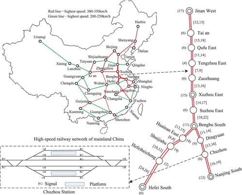
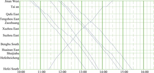
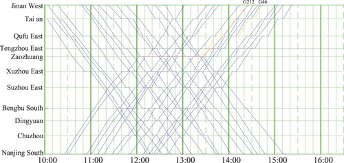
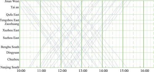
We consider a time horizon of 6.5 h, from 10:00 to 16:30. Based on the actual timetable in effect in 2015, a total of 36 trains are considered in our rescheduling, including 29 trains (15 inbound and 14 outbound) running between Jinan and Nanjing, and 7 trains (6 inbound and 1 outbound) running between Jinan and Hefei. As mentioned in Section 1.2, this considered railway line has 1266 time-independent arcs. Therefore, the rescheduling problem for this case has 17,774,640 ($1266\times 390\times 36$) variables. Note that we only consider trains departing within the 3-h period from 10:00 to 13:00, because we want to ensure that trains can more or less finish their journey within our 390-min horizon. The original timetables for these two lines are given in Figures 7 and 8. Note that three trains in Figure 7 depart from Jinan West station a few minutes before 10:00, so that we consider their running parts starting from Taian Station.

Figure 7. The original timetable for trains run between Jinan and Nanjing.

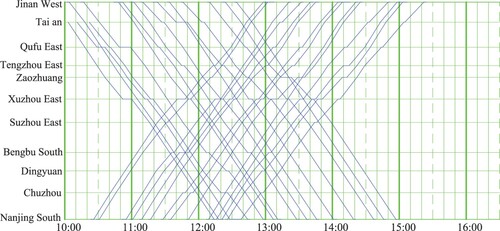
Figure 8. The original timetable for trains run between Jinan and Hefei.

We assume three kinds of disruption: (a) segment blockage, (b) station track blockage and (c) both segment and station track blockage. We vary the disruption location and duration to obtain various disruption scenarios. For the segment blockage, we assume that either both the tracks between Bengbu South and Dingyuan or those between Zaozhuang and Xuzhou East start to be blocked at 12:00, and the durations of the blockage could be 30, 60 or 90 min. Therefore, we obtain 6 disruption scenarios for the segment blockage situation. For the station track blockage, a siding in Tengzhou East Station is blocked for 30, 60 or 90 min from 12:00.

The train-running time in each segment is shown by a bracket beside each segment in Figure 6, the first and second numbers in each bracket are the running times for a high-speed train and a medium-speed train, respectively. Note that since only high-speed trains with a speed of 300–350 km/h run on the considered railway network, we change part of the high-speed trains to medium-speed trains by increasing their running time in a segment to test a more general case where multiple types of trains run on the same network. We assume the running times for inbound and outbound trains of the same type in the same segment are the same. If a train passes a station without stopping, we assume the passing time is 1 min, and if it stops at a station, the required time is assumed to be 3 min, including 1 min for passing and 2 min for dwelling. The arrival and departure headway time between two consecutive trains in a segment in the same direction is set to 3 min. The initial value of the penalty parameter ρ is set to 10, and the values of parameters γ and β to update the parameter ρ are set to 0.5 and 1.4, respectively. The initial Lagrangian multipliers ν and α are set to zero. We set a relatively large train cancelation penalty $C_k^0$ in the case study to prevent train cancelation, so that we do not cancel trains in the test.

5.2. Computational results

5.2.1. The efficiency of the ADMM algorithm

We test the efficiency of the ADMM algorithm on the segment blockage (scenario (a)). In scenario (a), we assume different disruption scenarios by varying the location and duration of the disruption. One disruption location is the segment between Bengbu South and Dingyuan (numbered 1), and the other is the segment between Zaozhuang and Xuzhou East (numbered 2). Both of these two disruptions are assumed to last for 30, 60 and 90 min. Therefore, we use a bracket to describe each disruption scenario in Table 2, where the first number (1 or 2) denotes the disruption location and the second number denotes the disruption duration.

Table 2. Computational results for different disruption scenarios when trains in both directions are rescheduled simultaneously.

Scenarios	Deviation (min)	Disrupted trains	Seriously disrupted trains	Gap	Iterations
(1, 30)	1443	30	6	0.6	10
(1, 60)	3854	31	11	25	17
(1, 90)	6001	32	16	6	12
(2, 30)	1432	29	5	2	8
(2, 60)	3671	30	12	18	15
(2, 90)	7581	31	20	13	16

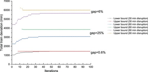
The solution of each disruption scenario is given in Table 2, where the second column contains the total train arrival deviations (objective), while the third and fourth columns show the number of disrupted trains (those for which the total deviation is positive) and the number of seriously disrupted trains (those for which the total deviation is at least 100 min), the fifth column is the gap between the solution obtained by ADMM and the lower bound obtained by LR, and the last column is number of iterations to obtain the best feasible solution within 20 steps. We limit the iteration step to 20 in the case study. From Table 2, we can see that ADMM can obtain a feasible solution for each disruption scenario within several iterations. If the disruption duration is longer, the train deviation is larger, and more trains are affected by the disruption. Most of the trains have a deviation because we change some high-speed trains to medium-speed trains by increasing their running time in a segment as mentioned before. However, this kind of deviation is usually small. Thus, we can focus on the seriously disrupted trains (column four) to see the influence of a disruption. We also can find that the blockage of segment between Zaozhuang and Xuzhou East has more serious influence on train operations than that of segment between Bengbu South and Dingyuan, because the latter blockage has less influence on the trains operated on the Jinan–Hefei line. For most disruption scenarios, the gap is below or around 10%, and the average gap is 10.8%. However, the gaps of some scenarios are relatively large, e.g. 25% for the scenario (1, 60). We can reduce this gap by trying different initial values of parameter ρ, which will be analyzed in section 5.2.3. We take the disruption scenarios (1, 30), (1, 60) and (1,90) as an example to show the convergence trend of the upper-bound and lower-bound solution in Figure 9. The computational time for each iteration is approximately 56 sec.

Figure 9. The gap between the upper bound solution obtained by ADMM and the lower bound obtained by LR for disruption scenarios (1, 30), (1,60) and (1,90).

The disposition timetable obtained by ADMM for disruption scenario (1, 90) is given in Figure 10. We can see that all the disrupted trains are stopped at the nearest station adjacent to the disruption location. In total, seven outbound trains are stopped at Bengbu South Station to wait for the end of the disruption, although there are normally only five station tracks available for outbound trains. Trains in both directions are allowed to share tracks in a station during a disruption, and Bengbu South has 11 station tracks in total, so the number of stopped trains is not limited to five. Therefore, the arrival delay for some trains at Bengbu South decreases. This is also the case at Dingyuan Station.

Figure 10. The disposition timetable for disruption scenario (a) when sidings are shared.

5.2.2. Strategy comparison

(1) Segment blockage: disruption scenario (a)

To investigate the advantages of rescheduling trains in both directions simultaneously (sidings are shared), we also test the situation where trains in different directions are rescheduled separately (sidings are not shared). That is, sidings on one side of the maintracks are used by trains traveling in one direction, and sidings on the other side are used by trains traveling in the opposite direction. All the other parameters maintain the same values as previously.

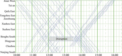
The solution for each disruption scenario is given in Table 3. The disposition timetable for the obtained solution of disruption scenario (1, 90) is illustrated in Figure 11.

Figure 11. The disposition timetable for disruption scenario (a) when sidings are separately used.

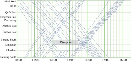
Table 3. Computational results for different disruption scenarios when trains in two directions are rescheduled separately.

Scenarios	Deviation (min)	Disrupted trains	Seriously disrupted trains	Iterations
(1, 30)	1435	30	6	7
(1, 60)	3714	31	11	11
(1, 90)	6659	32	16	16
(2, 30)	1432	29	5	9
(2, 60)	4226	31	13	20
(2, 90)	8491	32	20	20

Comparing the feasible solution obtained in the previous subsection (5.2.1) with that obtained here, we can see that the objective values (deviations) of most disruption scenarios increase when sidings are separately used, especially for disruption scenarios with a longer duration, e.g. 90 min. This is because the capacity of some stations becomes tighter when a longer blockage occurs. The most important difference between these two strategies is that when trains in both directions are rescheduled simultaneously, more trains can continue their journey before the disruption location because more station capacity is available to them. From Figure 11, we can see that only five outbound trains are stopped at Bengbu South to wait for the end of the disruption when sharing sidings are not allowed, because only five station tracks are allocated to outbound trains normally, as mentioned previously. This is quite different from the case in Figure 10, where we do not allow trains traveling in both directions to share sidings in a station. Therefore, the number of trains waiting in a station, e.g. Bengbu South, cannot exceed the station capacity (five). Meanwhile, the other two trains waiting at Bengbu South in Figure 10 have to stop at the previous station (Suzhou East) to wait for the end of the disruption. As a result, compared with the previous case, these two trains are delayed more when they arrive at Bengbu South. From disruption scenarios (1,90) and (2,90), we can conclude that the total train-deviation cost can be reduced by 11% and 12%, respectively, if trains traveling in different directions are rescheduled simultaneously and allowed to share sidings.

(2) Station-track blockage: disruption scenario (b)

In a disruption where some tracks in a station are blocked, the capacity of the station decreases significantly. Therefore, trains may be delayed due to the disruption. However, if we allow trains traveling in both directions to share the residual available sidings in the disrupted station, the influence of the disruption on train operations will be reduced. To illustrate the efficiency of the two siding-usage strategies, we compare the results obtained by allowing and forbidding the sharing of sidings in disruption scenario (b). In this scenario, we assume that the siding provided at platform 1 is temporarily blocked from 12:00 in Tengzhou East Station (see Figure 12) and lasts for 30, 60 or 90 min, respectively. Therefore, this platform track cannot be used by trains during the disrupted period. As Tengzhou East only has two main tracks (without platforms) and two sidings (with platforms), the influence of this disruption is significant if trains traveling in both directions are required to separately use tracks in this station. Specifically, inbound trains that have a planned stop at the siding provided at platform 1 cannot stop at this station to board and alight passengers during the disruption.

Figure 12. The disruption scenario in Tengzhou East Station.

If we do not allow high-speed trains to skip a station at which they are scheduled to stop, inbound trains with a planned stop at this station may suffer a large delay. All the parameters keep the same values as previously. We reschedule trains in these disruption scenarios, and the feasible solution obtained by ADMM for each disruption scenario is shown in Table 4. In the second column, the first number (3) in the bracket is the disruption location Tengzhou East, and the second number again is the duration of a disruption. The fourth column (DT) and fifth column (SDT) are the disrupted trains (i.e. the total deviation is positive) and seriously disrupted trains (i.e. the total deviation is at least 100 min), respectively. We can see that if inbound trains are allowed to sharing sidings in the disrupted station, they are not affected by the disruption. Note that the 976-min deviation is caused by the changing of some high-speed trains to medium-speed trains for our test purpose instead of disruption. Therefore, the deviations keep the same either the disruption lasts 30, 60 or 90 min in the simultaneously rescheduling case in Table 4. The train deviations are larger when we separately reschedule inbound and outbound trains (sharing sidings are not allowed) than those when we simultaneously reschedule trains for all disruption scenarios. The number of seriously disrupted trains is small compared with the segment blockage, but it increases in the separately rescheduling strategy. The computational time for train rescheduling in a station track blockage is shorter (approximately 450 sec) than that in segment blockage, i.e. fewer iterations are required to obtain a stable feasible solution for a disruption scenario.

Table 4. Computational results for different disruption scenarios in a station-track blockage.

Strategies	Scenarios	Deviation (min)	DT	SDT	Iterations
	(3, 30)	976	28	3	8
Simultaneously	(3, 60)	976	28	3	8
	(3, 90)	976	28	3	8
	(3, 30)	1040	27	3	8
Separately	(3, 60)	1204	27	4	8
	(3, 90)	1574	28	6	8

The disposition timetable for disruption scenario (3, 90) is shown in Figure 13. We have not shown all of the train numbers in the figure for simplicity. We can see that trains $G212$ and $G46$ stop at Zaozhuang, the station preceding Tengzhou East, for a long time, because these two trains have a planned stop at the disrupted station (Tengzhou East); see the red line and orange line in Figure 13. As we do not allow inbound trains to share the station tracks normally used by the outbound trains, these two trains cannot use the only residual track provided at a platform (i.e. the track at platform (2) in Tengzhou East Station. Therefore, they have to wait until the disruption ends, and then allow passengers to board and alight on the siding provided at platform 1.

Figure 13. The disposition timetable for disruption scenario (b) without sharing sidings.

For disruption scenario (b), we can also perform rescheduling of trains in both directions simultaneously by allowing trains in both directions to share sidings in a station. The values of all of the parameters are kept the same as those in the case where sharing sidings is not allowed. The solution for each disruption scenario is also given in Table 4 (simultaneously). The disposition timetable for disruption scenario (3, 90) is shown in Figure 14. As we allow inbound trains to share the sidings usually used by outbound trains, inbound trains can use the siding at platform 2 to allow passengers to board and alight when the track provided at platform 1 is blocked in Tengzhou East Station. As a result, trains $G212$ and $G46$ do not need to stop at Zaozhuang Station to wait for the disruption to end; see Figure 14.

Figure 14. The disposition timetable for disruption scenario (b) with sharing sidings.

Compared with the solution obtained by not allowing the sharing of sidings, the objective value here decreases, especially for long disruptions, i.e. the deviation of scenario (3, 90) increases 598 min. From this comparison, we can see that allowing trains in both directions to share sidings when some station tracks are blocked can significantly reduce the delay of disrupted trains.

(3) Both segment blockage and station-track blockage: disruption scenario (c)

We also test the disruption situation where both segment blockage and station-track blockage occur. We assume that one disruption is that both tracks in the segment between stations Bengbu South and Dingyuan are blocked from 12:00 with a duration of 60 min, and the other disruption is that the inbound siding in Tengzhou East Station is blocked from 12:00 and with various durations (30, 60, 90 and 120 min). We assume that both of the two disruptions occur at the same time because it is more complicated when two disruptions occur at different times. In the latter case, the information of two disruptions is available sequentially, so that the train rescheduling should be updated when the information of each disruption is available. We refer interested readers to Zhu, Goverde, and Quaglietta (2018) for train rescheduling in multiple simultaneous disruptions. Our test results are given in Table 5. Here a triple is used to denote a disruption scenario, where the first number means the segment blockage is in the segment between Bengbu South and Dingyuan, the second number is the duration of the segment blockage, and the last number is the duration of siding blockage at Tengzhou East.

Table 5. Computational results for different disruption scenarios in both a station track and a segment blockage.

Strategies	Scenarios	Deviation (min)	DT	SDT	Iterations
	(1, 60, 30)	3854	31	11	17
Simultaneously	(1, 60, 60)	3854	31	11	17
	(1, 60, 90)	3854	31	11	17
	(1, 60, 120)	3854	31	11	17
	(1, 60, 30)	3778	30	11	11
Separately	(1, 60, 60)	3942	30	12	11
	(1, 60, 90)	4155	31	13	11
	(1, 60, 120)	4459	31	14	12

We can see that, when we reschedule inbound and outbound trains simultaneously (allowing trains in both directions to share sidings), the station track blockage has no influence on the final solution, and only the segment blockage is in effect. This is because the station capacity of Tengzhou East is enough even an inbound siding is blocked. However, when we reschedule inbound and outbound trains separately where sharing siding is not allowed, both the two disruptions affect the solution. The total train deviation increases with the increase of the duration of the station-track blockage when the duration of the segment blockage is fixed.

5.2.3. Sensitivity analysis of parameter ρ

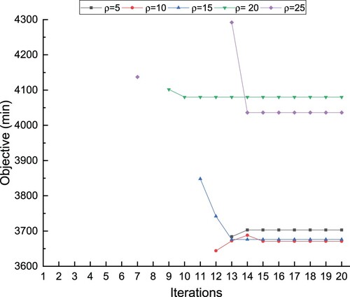
In the ADMM algorithm, the penalty parameter ρ affects the final solution. Although we have varied the value of parameter ρ in the iterative procedure, the original value of ρ may still affect the solutions. Thus, we analyze the influence of the original value for parameter ρ on the iterative solutions in this section by varying original ρ. We take the disruption scenario where the double tracks in the segment between Zaozhuang and Xuzhou East are blocked as an example. The start time of the disruption is 12:00, and it lasts 60 and 90 min, respectively. Except for the value of parameter ρ varying, all other parameters keep the same values as before. Trains in both directions are rescheduled simultaneously and sharing sidings is allowed.

The solutions for 20 iterations are given in Figures 15 (90-min disruption) and 16 (60-min disruption). In these two figures, if the solution of a certain iteration is infeasible, it is not marked. After several iterations, ADMM can find a stable feasible solution with an initial value of parameter ρ from 5 to 25. From the two figures, we can see that if a large value of parameter ρ is used as the initial value, a feasible solution can be found earlier (less iterations are required); however, the feasible solutions tend to be worse. Therefore, a trade-off exists between the number of iterations to find a feasible solution and the final solution quality. But the final feasible solution for $\rho =10$ is worse than that for either $\rho =20$ or $\rho =25$ in Figure 15. This may be because of the selected values of parameters γ and β in the Equation (24(24) ${\rho }^{\theta +1}=\{\begin{array}{ll}{\rho }^{\theta }& \text{if }|p{r}^{\theta }|\le \gamma |p{r}^{\theta -1}|\\ \beta \times {\rho }^{\theta }& \text{if }|p{r}^{\theta }|>\gamma |p{r}^{\theta -1}|\end{array}$(24) ) to update the value of ρ. To this end, ADMM cannot ensure to obtain a better solution with a smaller initial value of ρ, and we can try various initial values of ρ to choose a better final solution if possible.

Figure 15. The solution obtained in each iteration for different initial values of parameter ρ with a 90-min disruption.

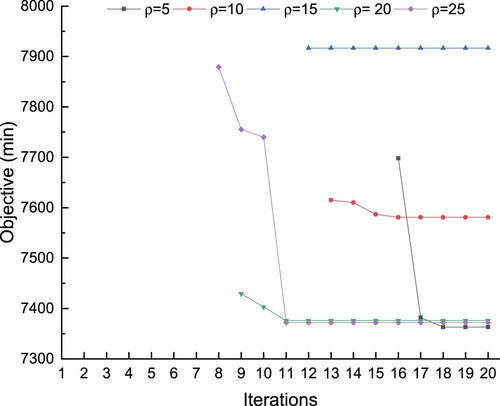
Figure 16. The solution obtained in each iteration for different initial values of parameter ρ with a 60-min disruption.

6. Conclusion and further research

In this paper, we studied the real-time train rescheduling of double-track high-speed railways in a highly disrupted situation. We allowed trains traveling in both directions to share sidings in a station if it was technically possible. Therefore, we rescheduled trains in both directions simultaneously to reduce the influence of a disruption on train operations. The railway line was considered at a meso-level by a space-time network, and the train routing in stations was considered. Based on the space-time network, an ILP model was formulated to solve the problem. Due to the complexity of our meso-level train rescheduling model, we introduced the ADMM algorithm to decompose the whole model into a series of easy-to-solve subproblems. This enables each subproblem to be regarded as a shortest-path searching problem, which can be efficiently solved by dynamic programming. To evaluate the quality of ADMM in solving the train-rescheduling problem, we obtained a lower-bound solution by LR. The real-world instance of the Jinan-Nanjing high-speed railway line and the Bengbu–Hefei intercity high-speed line was chosen to test our model and algorithms. Although we focused on high-speed railways, our approach can also be applied to conventional railways.

In our test, the ADMM algorithm proved quite efficient in finding a good feasible solution within several iterations for real-world train-rescheduling problems. Specifically, we found feasible solutions for the considered railway network with 36 trains with an average gap of 10.8% from the lower-bounds, in less than 20 iterations on a personal desktop in scenarios with complete blockage of a segment. For a station-track blockage, a good feasible solution could be found in even shorter computational time (less iterations). These results demonstrate that our approach enhances the scalability of solving train rescheduling on large networks with long-time horizons at a mesoscopic level.

In addition, we compared the solution obtained by simultaneous rerouting with that obtained by one-direction rerouting either in a segment blockage or a station track blockage. We found that the total train-deviation cost was much smaller in the simultaneous rerouting case in most disruption scenarios. Specifically, the total train-deviation cost decreased by 11% and 12% for scenarios (1,90) and (2,90) in the segment blockage situation, because disrupted trains could travel further to the nearest stations adjacent to the disruption area by sharing sidings usually reserved for trains traveling in the opposite direction. In a station-track blockage, the total train-deviation cost was reduced even more because other tracks in the disrupted stations were made available. Therefore, we conclude that rescheduling trains in both directions simultaneously (share sidings) is an important way to reduce the train deviation during a blockage. Railway managers and dispatchers could consider this strategy to reduce the influence of a disruption. However, the computational time for some disruption cases with a 6.5-h time horizon is still long. Thus, our approach still faces difficulties in solving a real-time problem with a long-time horizon and a large number of trains because our dynamic algorithm needs to search numerous possible paths for each train. However, this problem can be eased by using a beam search algorithm (Zhou and Zhong 2007) and parallel computing.

Several directions for further research are available. First, in this study of the case of a large disruption, we only rescheduled train timetables. However, an integrated method to consider the rescheduling of both the train timetable and the rolling stock is necessary. Second, we assumed that the disruption information was known in advance. It will be interesting to take the uncertain duration of a disruption into account. Third, our selection of suitable initial value for parameter ρ and values for parameters β and γ to update ρ in the ADMM algorithm were solely based on preliminary tests. A theoretical analysis of them would be assist to strengthen the convergence of the ADMM algorithm. Fourth, we assume that the running time of a train in a segment is fixed, but it would be better to let trains vary their running speeds in a segment. Finally, it is interesting to take the passenger flow into account when rescheduling trains, which can partly refer to our recent study on passenger-oriented train scheduling (Zhan, Wong, and Lo 2020) and rescheduling (Zhan et al. 2021).

Acknowledgments

The work was supported by a grant from the Research Grants Council of the Hong Kong Special Administrative Region, China (Project No. [T32-101/15-R]), the National Natural Science Foundation of China (NSFC) (No.71701174), the Fundamental Research Funds for the Central Universities (No.2682017CX020), the Key Scientific and Technological Project of Henan Province (No. 182102310799), the Foundation of Henan Educational Committee (No. 18A580003) and Beijing Municipal Natural Science Foundation (No.L181007). The first author was supported by the Hong Kong Scholar Scheme 2017. The second author was supported by the Francis S Y Bong Endowed Professorship in Engineering.

Disclosure statement

No potential conflict of interest was reported by the author(s).

Additional information

Funding

The work was supported by a grant from the Research Grants Council of the Hong Kong Special Administrative Region, China (Project No. [T32-101/15-R]), the National Natural Science Foundation of China (NSFC) [grant number 71701174], the Fundamental Research Funds for the Central Universities [grant number 2682017CX020], the Key Scientific and Technological Project of Henan Province [182102310799], the Foundation of Henan Educational Committee [grant number 18A580003] and Beijing Municipal Natural Science Foundation [grant number L181007]. The first author was supported by the Hong Kong Scholar Scheme 2017. The second author was supported by the Francis S Y Bong Endowed Professorship in Engineering.

References

- Albrecht, A. R., D. M. Panton, and D. H. Lee. 2013. “Rescheduling Rail Networks with Maintenance Disruptions Using Problem Space Search.” Computers & Operations Research 40 (3): 703–712.
- Arne Hansen, Ingo. 2008. Railway Timetable & Traffic: Analysis, Modelling, Simulation. Hamburg: Eurailpress.
- Boyd, Stephen, Neal Parikh, Eric Chu, Borja Peleato, and Jonathan Eckstein. 2011. “Distributed Optimization and Statistical Learning Via the Alternating Direction Method of Multipliers.” Foundations and Trends in Machine Learning 3 (1): 1–122.
- Brucker, Peter, Silvia Heitmann, and Sigrid Knust. 2002. “Scheduling Railway Traffic At a Construction Site.” OR Spectrum 24: 19–30.
- Cacchiani, Valentina, Dennis Huisman, Martin Kidd, Leo Kroon, Paolo Toth, Lucas Veelenturf, and Joris Wagenaar. 2014. “An Overview of Recovery Models and Algorithms for Real-time Railway Rescheduling.” Transportation Research Part B: Methodological 63: 15–37.
- Caimi, Gabrio, Dan Burkolter, Thomas Herrmann, Fabian Chudak, and Marco Laumanns. 2009. “Design of a Railway Scheduling Model for Dense Services.” Networks and Spatial Economics 9 (1): 25–46.
- Caprara, Alberto, Matteo Fischetti, and Paolo Toth. 2002. “Modeling and Solving the Train Timetabling Problem.” Operations Research 50 (5): 851–861.
- Corman, Francesco, and Andrea D'Ariano. 2012. “Assessment of Advanced Dispatching Measures for Recovering Disrupted Railway Traffic Situations.” Transportation Research Record 2289 (1): 1–9.
- Corman, Francesco, Andrea D'Ariano, Ingo A. Hansen, Dario Pacciarelli, and Marco Pranzo. 2011. “Dispatching Trains During Seriously Disrupted Traffic Situations”. In Networking, Sensing and Control (ICNSC), 2011 IEEE International Conference on, 323–328. Delft: IEEE.
- Corman, Francesco, and Lingyun Meng. 2015. “A Review of Online Dynamic Models and Algorithms for Railway Traffic Management.” Intelligent Transportation Systems, IEEE Transactions on 16 (3): 1274–1284.
- D'Ariano, Andrea, Lingyun Meng, Gabriele Centulio, and Francesco Corman. 2019. “Integrated Stochastic Optimization Approaches for Tactical Scheduling of Trains and Railway Infrastructure Maintenance.” Computers & Industrial Engineering 127: 1315–1335.
- Dollevoet, Twan, Francesco Corman, Andrea D'Ariano, and Dennis Huisman. 2014. “An Iterative Optimization Framework for Delay Management and Train Scheduling.” Flexible Services and Manufacturing Journal 26 (4): 490–515.
- Fang, Wei, Shengxiang Yang, and Xin Yao. 2015. “A Survey on Problem Models and Solution Approaches to Rescheduling in Railway Networks.” Intelligent Transportation Systems, IEEE Transactions on 16 (6): 2997–3016.
- Ghaemi, Nadjla, Oded Cats, and Rob M. P. Goverde. 2017. “A Microscopic Model for Optimal Train Short-turnings During Complete Blockages.” Transportation Research Part B: Methodological 105 (Supplement C): 423–437.
- Ghaemi, Nadjla, Oded Cats, and Rob M. P. Goverde. 2018. “Macroscopic Multiple-station Short-turning Model in Case of Complete Railway Blockages.” Transportation Research Part C: Emerging Technologies 89: 113–132.
- Hirai, Chikara, Taketoshi Kunimatsu, Norio Tomii, Shigeki Kondou, and Motoshi Takaba. 2009. “A Train Stop Deployment Planning Algorithm Using a Petri-net-based Modelling Approach.” Q. Rep. RTRI 50 (1): 8–13, doi:10.2219/rtriqr.50.8
- Jiang, Feng, Valentina Cacchiani, and Paolo Toth. 2017. “Train Timetabling by Skip-stop Planning in Highly Congested Lines.” Transportation Research Part B: Methodological 104: 149–174.
- Kang, Liujiang, Jianjun Wu Huijun Sun, Xiaoning Zhu, and Ziyou Gao. 2015a. “A Case Study on the Coordination of Last Trains for the Beijing Subway Network.” Transportation Research Part B: Methodological 72: 112–127.
- Kang, Liujiang, Jianjun Wu Huijun Sun, Xiaoning Zhu, and Bo Wang. 2015b. “A Practical Model for Last Train Rescheduling with Train Delay in Urban Railway Transit Networks.” Omega 50: 29–42.
- Kang, Liujiang, and Qiang Meng. 2017. “Two-phase Decomposition Method for the Last Train Departure Time Choice in Subway Networks.” Transportation Research Part B: Methodological 104: 568–582.
- Kang, Liujiang, Xiaoning Zhu, Huijun Sun, Jakob Puchinger, Mario Ruthmair, and Bin Hu. 2016. “Modeling the First Train Timetabling Problem with Minimal Missed Trains and Synchronization Time Differences in Subway Networks.” Transportation Research Part B: Methodological 93: 17–36.
- Kang, Liujiang, Xiaoning Zhu, Huijun Sun, Jianjun Wu, Ziyou Gao, and Bin Hu. 2019. “Last Train Timetabling Optimization and Bus Bridging Service Management in Urban Railway Transit Networks.” Omega 84: 31–44.
- Kecman, Pavle, Francesco Corman, Andrea D'Ariano, and Rob Goverde. 2013. “Rescheduling models for railway traffic management in large-scale networks.” Public Transport 5 (1–2): 95–123.
- Kliewer, Natalia, Taieb Mellouli, and Leena Suhl. 2006. “A Time Cspace Network Based Exact Optimization Model for Multi-depot Bus Scheduling.” European Journal of Operational Research 175 (3): 1616–1627.
- Kroon, Leo G, H Edwin Romeijn, and Peter J Zwaneveld. 1997. “Routing Trains Through Railway Stations: Complexity Issues.” European Journal of Operational Research 98 (3): 485–498.
- Lamorgese, Leonardo, Carlo Mannino, and Mauro Piacentini. 2016. “Optimal Train Dispatching by Benders-like Reformulation.” Transportation Science 50 (3): 910–925.
- Louwerse, Ilse, and Dennis Huisman. 2013. “Adjusting a Railway Timetable in Case of Partial Or Complete Blockades.” European Journal of Operational Research 235 (3): 583–593.
- Luan, Xiaojie, Jianrui Miao, Lingyun Meng, Francesco Corman, and Gabriel Lodewijks. 2017. “Integrated Optimization on Train Scheduling and Preventive Maintenance Time Slots Planning.” Transportation Research Part C: Emerging Technologies 80: 329–359.
- Meng, Lingyun, and Xuesong Zhou. 2011. “Robust Single-track Train Dispatching Model Under a Dynamic and Stochastic Environment: a Scenario-based Rolling Horizon Solution Approach.” Transportation Research Part B: Methodological 45 (7): 1080–1102.
- Meng, Lingyun, and Xuesong Zhou. 2014. “Simultaneous Train Rerouting and Rescheduling on An N-track Network: A Model Reformulation with Network-based Cumulative Flow Variables.” Transportation Research Part B: Methodological 67: 208–234.
- Olsen, Nils, Natalia Kliewer, and Lena Wolbeck. 2020. “A Study on Flow Decomposition Methods for Scheduling of Electric Buses in Public Transport Based on Aggregated Time Cspace Network Models.” Central European Journal of Operations Research. doi:10.1007/s10100-020-00705-6.
- Pellegrini, Paola, Grégory Marlière, and Joaquin Rodriguez. 2014. “Optimal Train Routing and Scheduling for Managing Traffic Perturbations in Complex Junctions.” Transportation Research Part B: Methodological 59: 58–80.
- Xu, Peijuan, Francesco Corman, Qiyuan Peng, and Xiaojie Luan. 2017. “A Train Rescheduling Model Integrating Speed Management During Disruptions of High-speed Traffic Under a Quasi-moving Block System.” Transportation Research Part B: Methodological 104: 638–666.
- Steinzen, Ingmar, Vitali Gintner, Leena Suhl, and Natalia Kliewer. 2010. “A Time-space Network Approach for the Integrated Vehicle- and Crew-scheduling Problem with Multiple Depots.” Transportation Science 44 (3): 367–382.
- Van Aken, Sander, Nikola Bešinović, and Rob M. P. Goverde. 2017. “Designing Alternative Railway Timetables Under Infrastructure Maintenance Possessions.” Transportation Research Part B: Methodological 98: 224–238.
- Vansteenwegen, Pieter, Thijs Dewilde, Sofie Burggraeve, and Dirk Cattrysse. 2016. “An Iterative Approach for Reducing the Impact of Infrastructure Maintenance on the Performance of Railway Systems.” European Journal of Operational Research 252 (1): 39–53.
- Veelenturf, Lucas P, Martin P Kidd, Valentina Cacchiani, Leo G Kroon, and Paolo Toth. 2015. “A Railway Timetable Rescheduling Approach for Handling Large-scale Disruptions.” Transportation Science 50 (3): 841–862.
- Wang, Wenshan, Meng Xu, Paolo Guarneri, and Georges Fadel. 2012. “A Consensus Optimization via Alternating Direction Method of Multipliers for Network Target Coordination”. In 12th AIAA Aviation Technology, Integration, and Operations (ATIO) Conference and 14th AIAA/ISSMO Multidisciplinary Analysis and Optimization Conference, 5552.
- Wüst, Raimond, Stephan Bütikofer, Severin Ess, Claudio Gomez, Albert Steiner, Marco Laumanns, and Jacint Szabo. 2019. “Maintenance Timetable Planning Based on Mesoscopic Infrastructure and the Transport Service Intention.” Journal of Rail Transport Planning & Management11100–11146.
- Yao, Yu, Xiaoning Zhu, Hongyu Dong, Shengnan Wu Hailong Wu, Lu Carol Tong, and Xuesong Zhou. 2019. “ADMM-based Problem Decomposition Scheme for Vehicle Routing Problem with Time Windows.” Transportation Research Part B: Methodological 129: 156–174.
- Zhan, Shuguang, Leo G. Kroon, Lucas P. Veelenturf, and Joris Wagenaar. 2015. “Real-time High-speed Train Rescheduling in Case of a Complete Blockade.” Transportation Research Part B: Methodological78: 182–201.
- Zhan, Shuguang, Leo G. Kroon, Jun Zhao, and Qiyuan Peng. 2016. “A Rolling Horizon Approach to the High Speed Train Rescheduling Problem in Case of a Partial Segment Blockage.” Transportation Research Part E: Logistics and Transportation Review 95: 32–61.
- Zhan, Shuguang, S. C. Wong, and S. M. Lo. 2020. “Social Equity-based Timetabling and Ticket Pricing for High-speed Railways.” Transportation Research Part A: Policy and Practice 137: 165–186.
- Zhan, Shuguang, S. C. Wong, Qiyuan Peng, and S. M. Lo. 2019. “Train Stop Deployment Planning in the Case of Complete Blockage: An Integer Linear Programing Model.” Journal of Transportation Safety & Security 1–27, doi:10.1080/19439962.2019.1645773
- Zhan, S., S. C. Wong, P. Shang, Q. Peng, J. Xie, and S. M. Lo. 2021. “Integrated Railway Timetable Rescheduling and Dynamic Passenger Routing During a Complete Blockage.” Transportation Research Part B: Methodological 143: 86–123.
- Zhang, Yongxiang, Andrea D'Ariano, Bisheng He, and Qiyuan Peng. 2019a. “Microscopic Optimization Model and Algorithm for Integrating Train Timetabling and Track Maintenance Task Scheduling.” Transportation Research Part B: Methodological 127: 237–278.
- Zhang, Yongxiang, Qiyuan Peng, Yu Yao, Xin Zhang, and Xuesong Zhou. 2019b. “Solving Cyclic Train Timetabling Problem Through Model Reformulation: Extended Time-space Network Construct and Alternating Direction Method of Multipliers Methods.” Transportation Research Part B: Methodological 128: 344–379.
- Zhou, Wenliang, and Hualiang Teng. 2016. “Simultaneous Passenger Train Routing and Timetabling Using An Efficient Train-based Lagrangian Relaxation Decomposition.” Transportation Research Part B: Methodological 94: 409–439.
- Zhou, Xuesong, and Ming Zhong. 2007. “Single-track Train Timetabling with Guaranteed Optimality: Branch-and-bound Algorithms with Enhanced Lower Bounds.” Transportation Research Part B: Methodological 41: 320–341.
- Zhu, Yongqiu, and Rob M. P. Goverde. 2019. “Railway Timetable Rescheduling with Flexible Stopping and Flexible Short-turning During Disruptions.” Transportation Research Part B: Methodological 123: 149–181.
- Zhu, Yongqiu, Rob Goverde, and Egidio Quaglietta. 2018. “Railway timetable rescheduling for multiple simultaneous disruptions”. In CASPT 2018: 14th conference on advanced systems in public transport and TransitData 2018, Brisbane, Australia. http://resolver.tudelft.nl/uuid:1664b528-4e12-4745- bf87-a798a7e878ef.
- Zilko, Aurelius A, Dorota Kurowicka, and Rob M. P. Goverde. 2016. “Modeling Railway Disruption Lengths with Copula Bayesian Networks.” Transportation Research Part C: Emerging Technologies 68: 350–368.