Empirical analysis of scaled mixed itinerary-size weibit model for itinerary choice in a schedule-based railway network

Abstract

The mixed itinerary-size weibit (MISW) model was recently developed for predicting passengers’ itinerary-choice behaviors in a schedule-based railway network. It considers passengers’ heterogeneous perceptions and relaxes the independently and identically distributed assumptions of random utility models. However, this model has not been verified using real-world data. Moreover, it is assumed that passengers hold a negative perception of overlapping, but this assumption may not be suitable for all situations. Thus, this study proposes a scaled MISW model which includes a scale parameter to address this issue. We collected passenger ticket-booking data from the South China High-Speed Railway network and conducted an empirical analysis in which we compared the performances of the scaled MISW model and other models (i.e. the multinomial logit, multinomial weibit, and MISW models). According to the results, the scaled MISW model outperformed the other models in describing passengers’ choice behaviors in the railway network.

KEYWORDS:

• Scaled mixed itinerary-size weibit model
• empirical analysis
• itinerary choice
• high-speed railway

1. Introduction

High-speed railway (HSR) is being developed rapidly, and numerous studies on HSR have been conducted (Jou, Chien, and Wu 2013; Chou, Lu, and Chang 2014; Yilmaz and Ari 2017; Zhen, Cao, and Tang 2018; Pimentel, Nunes, and Couto 2018; Zhao and Zhao 2019; Zhang et al. 2020; Cacchiani, Qi, and Yang 2020; Zhan, Wong, and Lo 2020; Xie et al. 2021). HSR planning has been researched extensively, and it typically involves the simulation of passengers’ itinerary choices to assess planning results and improve planning (Zhou et al. 2020). To formulate such simulations for a schedule-based railway system, the mixed itinerary-size weibit (MISW) model was recently proposed (Xie et al. 2020).

The MISW model offers three theoretical advantages. First, it assumes that the random-error term follows the Weibull distribution, meaning that it compares itineraries in terms of the relative cost difference rather than the absolute cost difference. The absolute cost difference, which is used by logit-type models, may lead to overestimation of passengers’ perceptions of cost differences (Kitthamkesorn and Chen 2013). Second, the MISW model adopts a correction term (i.e. the itinerary-size (IS) factor, similar to the path-size factor suggested in Ben-Akiva and Bierlaire (1999) for the route overlap problem in path choice) to resolve the itinerary overlap problem. Third, random coefficients are included in the MISW model to address the heterogeneity in passengers’ perceptions. Xie et al. (2020) provided three numerical examples to support these advantages.

However, the MISW model assumes that the passengers place a negative value on the route overlap. In contrast, different opinions exist on the passengers’ perception of overlapping, and some studies (Hoogendoorn-Lanser and Bovy 2007; Anderson, Nielsen, and Prato 2017) have found the empirical evidence suggesting that passengers may have an opposite view. Hence, the MISW model’s assumption on route overlap may not be suitable for all situations, and thus this study proposes a scaled MISW model, which introduces a scale parameter into the present MISW model to capture passengers’ perceptions of route overlap. In this study, we collected HSR ticket-booking data from South China to calibrate and compare the scaled MISW model with a multinomial logit (MNL) model, a multinomial weibit (MNW) model, and an MISW model. The MISW and scaled MISW models have not been verified using real-world data, and these data have not yet been used in any itinerary-choice model. To the best of our knowledge, this is the first use of ticket-booking data to calibrate discrete-choice models designed to solve the China HSR itinerary-choice problem. The results revealed that the scaled MISW model is superior for describing passengers’ choice behaviors in an HSR network.

The rest of this paper is organized as follows. Section 2 provides a review of the weibit-type models, and Section 3 introduces the scaled MISW model. Section 4 presents a case study by using HSR ticket-booking data obtained from South China, and Section 5 discusses the empirical results. Our concluding remarks are given in Section 6.

2. Literature review

Route choices in a railway network are different from those in a road network because a railway network provides fewer departure times and routes than a road network (Tong and Richardson 1984). Therefore, ‘itinerary choice’ is used instead of ‘path choice’ in railway travel analysis to emphasize the two-dimensional nature of route choice in railway travel. Figure 1 clarifies the concept of an itinerary.

Figure 1. Illustration of the itinerary concept.

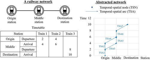
A train network is abstracted using temporal–spatial nodes (TSNs) and temporal–spatial arcs (TSAs). A TSN represents a single event, such as taking Train 1 to depart from the origin station. A TSA links two TSNs. Based on the passenger behavior, TSAs can be divided into in-train TSAs (e.g. TSA3 in Figure 1), wait TSAs (e.g. TSA1 in Figure 1), and transfer TSAs (e.g. TSA5 in Figure 1). We consider a transfer as having occurred when a passenger leaves one train and boards another. A TSA branch may form a feasible itinerary, for example, TSA1 → TSA3 → TSA5 → TSA6 → TSA7.

A schedule-based approach is more appropriate than a frequency-based approach for modeling railway itineraries, because it can consider the passenger’s decision to depart at a certain time and board a certain train (Hamdouch, Szeto, and Jiang 2014; Xie, Wong, and Lo 2017). This cannot be achieved using the frequency-based approach because it considers the average network performance and passenger characteristics (Nuzzolo, Russo, and Crisalli 2001). There are two approaches for establishing schedule-based itinerary-choice models: traditional utility-based methods and newly developed machine-learning methods. Sun et al. (2018) used machine-learning methods to predict the HSR itinerary choices from Shanghai to Beijing. These methods identify the patterns iteratively and extract rules from the data instead of assuming relationships between the choices and explanatory variables. Thus, although machine-learning methods may better predict passengers’ itinerary choices, their results are more difficult to interpret than those of utility-based methods, which consider socio-demographics and the attributes of choice alternatives in utility functions. Such interpretability is useful because it can help operators understand the underlying relationships and make decisions to improve railway network operations. Therefore, utility-based methods continue to be the main tools used by operators to model passenger-itinerary choices.

Utility-based models commonly form the following utility function (Equation (1)): (1) $U(\mathit{\beta }\text{,}\mathit{x})=V(\mathit{\beta }\text{, }\mathit{x})+\epsilon$(1)

The utility ($U$) of a choice is affected by the passengers’ perceptions $\mathit{\beta }$ and the cost $\mathit{x}$ paid for making this choice, and can be divided into two parts, namely the observed term $V(\mathit{\beta }\text{, }\mathit{x})$ and the unobserved term $\epsilon$. $\epsilon$ is assumed to follow a certain distribution, such as a Gumbel distribution (Dial 1971) or normal distribution (Daganzo and Sheffi 1977). The Gumbel distribution is most widely accepted and generates the MNL model and its variants (Van Nes, Hoogendoorn-Lanser, and Koppelman 2008; Lim and Kim 2016).

However, the MNL model has some drawbacks due to its use of the independently and identically distributed (IID) assumption (Sheffi 1985). The IID assumption considers trips of various lengths to be identical. For instance, although the absolute difference between two itineraries is 5 min, the relative difference varies. The MNL model focuses on the absolute difference and provides the same choice probabilities, regardless of whether the relative difference is 50% or 5%. In the first scenario, the two itineraries will be perceived significantly differently, but in the second scenario, the two itineraries will be perceived similarly. Thus, this length-specific perception variance is not captured by the MNL model. To capture this variance, Castillo et al. (2008) derived the MNW model by assuming that costs were Weibull-distributed, and Fosgerau and Bierlaire (2009) developed a similar model by assuming a multiplicative utility function that was a product of systematic utility and a random-error term. Kitthamkesorn and Chen (2014) later demonstrated that the MNW model resolved this failure of the MNL model by using numerical examples, and Fosgerau and Bierlaire (2009) used empirical data of trains, buses, and cars to illustrate the superiority of the MNW model. For the train dataset, Fosgerau and Bierlaire (2009) formulated three different utility functions and observed significant improvements in the log-likelihood of the MNW model relative to that of the MNL model in these three cases (the improvements in the log-likelihood ranged from 171.76–239.45). This result indicated that the weibit-type models may be more suitable than the logit-type models for studying itinerary choices in a train system. Another advantage of the MNW model is that its computational complexity is always similar to that of the MNL model. We can transform the systematic utility of the MNW model into the logarithmic form and apply traditional tools to the MNL model to estimate the MNW model (Castillo et al. 2008; Fosgerau and Bierlaire 2009). Due to these advantages, the MNW model has been applied to real-world cases, such as designing optimal expressway tolls (Kurauchi and Ido 2017).

Although the MNW model addresses the identically distributed assumption, it retains the independently distributed assumption, which is often violated by real-world correlation among itineraries, and scholars solve the correlation problem by including nesting structures in their models (Li et al. 2010; Hess et al. 2013) or by adding a correction term to the utility function, such as the C-logit model (Cascetta et al. 1996; Zhou, Chen, and Bekhor 2012), path-size logit model (Ben-Akiva and Bierlaire 1999; Chen et al. 2012), and path-size weibit (PSW) model (Kitthamkesorn and Chen 2013).

The PSW model relaxes the IID assumption, and the MISW model (Xie et al. 2020) was developed based on the PSW model to suit railway networks. Furthermore, the MISW model includes random coefficients to alleviate the problem of heterogeneity in passengers’ perceptions. Xie et al. (2020) provided numerical examples to demonstrate the superiority of the MISW model in solving problems related to length-specific perception variance, variance in coefficients, and overlapping itineraries. Although the abovementioned numerical analyses have revealed the advantages of the MISW model, it has yet to be applied in an empirical study. This study contributed to the literature by performing an empirical analysis of the MISW model in an HSR network. Moreover, thus far, ticket-booking data have not been used to analyze Chinese HSR itinerary choices with discrete-choice models. Hence, this study, which used HSR passenger ticket-booking data, filled this research gap.

Furthermore, the MISW model assumes that a negative perception exists regarding overlap. Although the evidence of this assumption can be commonly found in the road network, the present research on passengers’ perceptions of overlapping holds different opinions. Some studies (Yap, Cats, and van Arem 2018; Xie et al. 2020) have suggested a negative perception because the overlapping itineraries can be regarded as similar in the passengers’ opinions, and thus are less likely to be selected compared to the relatively independent itineraries. However, Hoogendoorn-Lanser and Bovy (2007) and Anderson, Nielsen, and Prato (2017) argued that the additional attractiveness of the overlap can compensate for the negative impact, and thus overlap can pose a positive impact on utility. For example, overlapping itineraries indicate more alternative routes to reach the destination, and the passengers may value this, given the risk of missing trains. Their empirical studies supported this argument. Besides, the overlapping part of the itineraries is commonly a route that connects two major terminals, and the railway company is more likely to offer better-than-average services (e.g. more serving staff onboard and diversified meal choices). Hence, passengers’ perceptions of itinerary overlap may vary among the different studied cases. This study suggests a new model, the scaled MISW model, to resolve the overlapping-perception problem existing in the MISW model.

3. Scaled mixed itinerary-size weibit model

This section describes the notation system and major assumptions of weibit-type models, and introduces the MNW model, which is the foundation of the scaled MISW model. Furthermore, the formulation of the scaled MISW model is described. Specifically, the advantages of weibit-type models are illustrated using two numerical examples.

3.1. Notation system

The elements, sets, and variables used in weibit-type models are defined in Table 1.

Table 1. Elements, sets, and variables used in weibit-type models.

Element	Description
$a$ or $a^{\mathrm{\prime }}$	Temporal-spatial arc (TSA)
$i$ or $i^{\mathrm{\prime }}$	Itinerary
Set	Description
${\mathit{A}}_i$	Set of TSAs belonging to $i$
$\mathit{I}$	Set of available itineraries
Variables	Description
$b_{ai}$	1 if itinerary $i$ uses TSA $a$, and 0 otherwise
$c_i$	Total perceived cost if $i$ is used
$N^{\text{I}}$	Number of itineraries
$t_a$	Time of $a$
${\check{U}}_i$	Disutility of $i$
${\mathit{x}}_i$	Vector of cost components of $i$
$\mathit{y}$	Vector of socio-demographics with mean $\overline{\mathit{y}}$ and standard deviation $\mathit{\sigma }$
$\text{Pro}{\text{b}}_i$	Probability of passengers selecting $i$
$\mathit{\beta }$	Vector of cost coefficients
${\omega }_i$	Itinerary-size factor for $i$
${\epsilon }_i$	Independent random-error term for $i$
$\xi$	Location parameter
$\gamma$	Shape parameter
$\tau$	Scale parameter of the itinerary-size factor
$\mathit{\theta }$	Matrix of factors revealing the effects of socio-demographics on ${\mathit{x}}_i$
$\tilde{\mathit{\theta }}$	Vector of constants for deciding $\mathit{\beta }$

3.2. Major assumptions

The following assumptions are made in this study.

1. Passengers have perfect information about the railway system. However, passengers’ perceptions are heterogenous, and components of utilities may not be fully included.

2. The perceived cost of itinerary $i\in \mathit{I}$, $c_i$, includes various costs (such as the elapsed time and the number of transfers) and is weighted based on passenger perceptions as follows (Equation (2)): (2) $c_i=\mathit{\beta }{\mathit{x}}_i,\mathrm{\forall }i\in \mathit{I}$(2) where $\mathit{\beta }$ is a coefficient vector that indicates the passengers’ preference for cost components, and ${\mathit{x}}_i$ is a vector of the cost components of itinerary $i$. Socio-demographics (e.g. age and gender) determine $\mathit{\beta }$ (Equation (3)): (3) $\mathit{\beta }=f(\mathit{y}\text{,}\mathit{\theta }\text{,}\stackrel{\mathbf{~}}{\mathit{\theta }})$(3) where $\mathit{y}$ is a vector of socio-demographics, $\mathit{\theta }$ is a factor matrix of $\mathit{y}$, and $\tilde{\mathit{\theta }}$ is a vector of constant values. This study assumes Equation (3) takes a linear form, and $\mathit{\beta }$ is given by Equation (4), as follows: (4) $\mathit{\beta }=\mathit{\theta }\mathit{y}+\tilde{\mathit{\theta }}$(4)

3. Trains have high punctuality.

4. Trains have adequate capacity, so that passengers can always board on their selected trains. The situation in which trains do not have adequate capacity is out of the scope of this study, and the future research will consider building itinerary choice models for this situation.

5. The railway system is run by a single operator. For example, the Passenger Transport Department of the China Railway Corporation is responsible for the operation of all HSR trains in China and passengers purchase tickets from this corporation, although the daily operations of different HSR trains are run by its different subsidiaries.

3.3. MNW model

The MNW model assumes that the independent random-error term ${\epsilon }_i$ of itinerary $i$ follows the Weibull distribution, location parameter $\xi \in [0,c_i)$, and shape parameter $\gamma \in (0,+\mathrm{\infty })$. The disutility function of the MNW model is defined as follows (Equation (5)): (5) ${\stackrel{⌣}{U}}_i=(c_i-\xi {)}^{\gamma }{\epsilon }_i,\mathrm{\forall }i\in \mathit{I}$(5)

Hence, the MNW model calculates the probability that a passenger will select itinerary $i$ as follows (Equation (6)): (6) $\text{Pro}{\text{b}}_i=\frac{{(c_i-\xi )}^{-\gamma }}{{\sum }_{i^{\mathrm{\prime }}\in \mathit{I}}{(c_{i^{\mathrm{\prime }}}-\xi )}^{-\gamma }},\mathrm{\forall }i\in \mathit{I}$(6)

For further details regarding the mathematical deduction, please refer to Castillo et al. (2008) and Kitthamkesorn and Chen (2014).

If disutility ${\stackrel{⌣}{U}}_i$ is positive, passengers should give something (e.g. time and money) if choosing itinerary $i$, whereas if disutility ${\stackrel{⌣}{U}}_i$ is negative, passengers would earn something (e.g. freedom and success in attending an important activity) if choosing itinerary $i$. Therefore, if disutility ${\stackrel{⌣}{U}}_i$ is greater, a passenger will be less likely to select itinerary $i$. According to Equations (2), (5), and (6), a positive element in $\mathit{\beta }$ means that if the respective cost component of itinerary $i$ is greater, cost $c_i$ and disutility ${\stackrel{⌣}{U}}_i$ are greater and itinerary $i$ is less likely being chosen. By contrast, a negative element in $\mathit{\beta }$ means that if the respective cost component of itinerary $i$ is greater, cost $c_i$ and disutility ${\stackrel{⌣}{U}}_i$ are smaller and itinerary $i$ is more likely being chosen.

To illustrate how the MNW model compares relative cost differences, Equation (6) is rewritten as Equation (7): (7) $\text{Pro}{\text{b}}_i=\frac{{(c_i-\xi )}^{-\gamma }}{{\sum }_{i^{\mathrm{\prime }}\in \mathit{I}}{(c_{i^{\mathrm{\prime }}}-\xi )}^{-\gamma }}=\frac{1}{{\sum }_{i^{\mathrm{\prime }}\in \mathit{I}}{\left(\frac{c_{i^{\mathrm{\prime }}}-\xi }{c_i-\xi }\right)}^{-\gamma }},\mathrm{\forall }i\in \mathit{I}$(7) where $\frac{c_{i^{\mathrm{\prime }}}-\xi }{c_i-\xi }$ indicates the corrected relative cost difference between two itineraries, $i$ and $i^{\mathrm{\prime }}$. In contrast, the MNL model accounts for the absolute cost difference $(c_i-c_{i^{\mathrm{\prime }}})$, such that it ignores how the overall itinerary cost influences passengers’ perception, as given by Equation (8): (8) $\text{Pro}{\text{b}}_i=\frac{e^{-c_i}}{{\sum }_{i^{\mathrm{\prime }}\in \mathit{I}}{e}^{-c_{i^{\mathrm{\prime }}}}}=\frac{1}{{\sum }_{i^{\mathrm{\prime }}\in \mathit{I}}{e}^{(c_i-c_{i^{\mathrm{\prime }}})}},\mathrm{\forall }i\in \mathit{I}$(8)

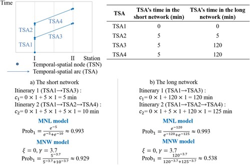
The two-itinerary example shown in Figure 2 is formulated for further demonstration. The coefficients for the in-vehicle time (IVT) and waiting time are both equal to 1. Following the assumption of Kitthamkesorn and Chen (2013), we set $\gamma =$ 3.7 and $\xi =0$. Although the absolute cost difference between the two itineraries is the same in both networks, the cost of Itinerary 2 is double that of Itinerary 1 in the short network, whereas the cost of Itinerary 2 is only 4.2% higher than that of Itinerary 1 in the long network. These two networks should not have the same likelihood of selecting Itinerary 1, but the same likelihood (0.993) is selected by the MNL model. In contrast, the MNW model considers the relative difference and suggests that the likelihood of selecting Itinerary 1 in the long network is lower than that in the short network.

Figure 2. Two-itinerary example. Note: The example networks were built based on the example of Kitthamkesorn and Chen (2013).

3.4. Scaled MISW model

The MISW model is proposed to relax the IID assumption and the assumption of homogeneity in passengers’ perceptions by including the IS factor and random coefficients. Xie et al. (2020) formulated the IS factor based on the original form of the path-size factor suggested by Ben-Akiva and Bierlaire (1999) as follows (Equation (9)): (9) ${\omega }_i=\sum _{a\in {\mathit{A}}_i}\frac{t_a}{{\sum }_{a^{\mathrm{\prime }}\in {\mathit{A}}_i}{t}_{a^{\mathrm{\prime }}}}\frac{1}{{\sum }_{i^{\mathrm{\prime }}\in \mathit{I}}{b}_{a{i}^{\mathrm{\prime }}}},\mathrm{\forall }i\in \mathit{I}$(9) where $t_a$ is the time of TSA $a$ ($a\in {\mathit{A}}_i$, ${\mathit{A}}_i$ comprises the TSAs belonging to itinerary $i$). The variable $b_{ai}$ equals 1 if TSA $a$ belongs to itinerary $i$, and is 0 otherwise. The ratio $\frac{t_a}{{\sum }_{a^{\mathrm{\prime }}\in {\mathit{A}}_i}{t}_{a^{\mathrm{\prime }}}}$ approximates the itinerary correlation, and $\sum _{i^{\mathrm{\prime }}\in \mathit{I}}{b}_{a{i}^{\mathrm{\prime }}}$ estimates how TSA $a$ affects the itinerary correlation.

This study adds a scale parameter ($\tau \in (-\mathrm{\infty },+\mathrm{\infty })$) to the disutility function of the MISW model to reflect the passengers’ perception of overlapping. The new disutility function can be expressed as follows (Equation (10)): (10) ${\check{U}}_i=\frac{{(c_i-\xi )}^{\gamma }}{{({\omega }_i)}^{\tau }}{\epsilon }_i,\mathrm{\forall }i\in \mathit{I}$(10)

This function yields a new choice model called the scaled MISW model. The MISW model without a scale parameter for the IS factor assumes that passengers hold a negative view regarding itinerary overlap (i.e. $\tau =1$), because passengers would consider the overlapping itineraries similar and thus are less likely to select the overlapping itineraries compared to the relatively independent itineraries. However, some studies (Hoogendoorn-Lanser and Bovy 2007; Anderson, Nielsen, and Prato 2017) argued that the additional attractiveness of the overlap (such as having more alternatives) may compensate for the negative impact in some cases, which was supported by empirical evidence. If the MISW model’s assumption on itinerary overlap does not meet the actual situation, the MISW model will give the incorrect estimation on choice probabilities. In contrast, the scaled MISW model can account for different passengers’ perception on itinerary overlap by setting a suitable $\tau$. Regarding itinerary overlap, when passengers hold a negative view, $\tau$ is positive; when passengers hold a positive view, $\tau$ is negative; and when passengers hold an indifferent view, $\tau$ is zero. In addition, a larger $\tau$ results in a larger disutility because ${\omega }_i\in (0,1]$, i.e. the attractiveness of overlapping itineraries decreases, and thus the probabilities of choosing overlapping itineraries decline.

If this model assumes that a few elements of passenger characteristics $\mathit{y}$ are independently normally distributed, (i.e. $\mathit{y}\sim \mathcal{N}(\overline{\mathit{y}}\text{, }{\mathit{\sigma }}^2)$), the probability of choosing itinerary $i\in \mathit{I}$ can be written as (11) $\text{Pro}{\text{b}}_i={\int }^{}\frac{{({\omega }_i)}^{\tau }{(c_i-\xi )}^{-\gamma }}{{\sum }_{i^{\mathrm{\prime }}\in \mathit{I}}{({\omega }_{i^{\mathrm{\prime }}})}^{\tau }{(c_{i^{\mathrm{\prime }}}-\xi )}^{-\gamma }}\times \frac{1}{\sqrt{2\pi {\mathit{\sigma }}^2}}{e}^{-\frac{{(\dot{\mathit{y}}-\overline{\mathit{y}})}^2}{2{\mathit{\sigma }}^2}}d\dot{\mathit{y}},\mathrm{\forall }i\in \mathit{I}$(11)

Note that $\mathit{y}$ can follow other distributions depending on various real scenarios, and the scaled MISW model can be calibrated using the simulated maximum likelihood estimation method.

To reveal the superiority of the scaled MISW model, a three-itinerary example (Xie et al. 2020) is presented in Figure 3.

Figure 3. Three-itinerary network. Note: The network of the three-itinerary example was built based on the example of Kitthamkesorn and Chen (2013).

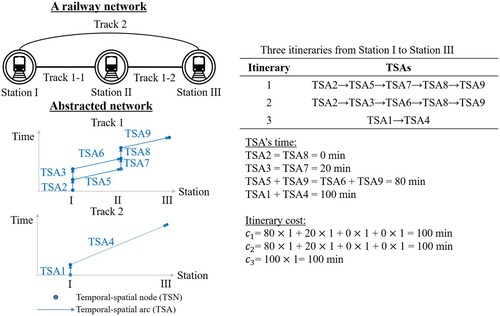
There are two rail tracks connecting Stations I and III. Track 1 is divided into two segments (Track 1-1 and Track 1-2) by Station II. To show train movements between these two track segments in Figure 3, the abstracted network is presented using two time-station figures, whose upper and lower parts represent Track 1 and Track 2, respectively. Two trains run on Track 1-1, and they are represented as TSA5 and TSA6. One train runs on Track 1-2, and it is represented as TSA9. One train runs on Track 2, and it is represented as TSA4. The itinerary cost consists of IVT, waiting time, and transfer time; the coefficients without variance are all equal to 1. For these three itineraries, the itinerary cost is set to be the same, that is, 100 min. As mentioned before, $\xi =$ 0 and $\gamma =$ 3.7. We vary the overlapping part ($t_{\text{OL}}=t_{\text{TSA}2}+t_{\text{TSA}8}+t_{\text{TSA}9}$) and calculate the respective itinerary-choice probabilities.

The MNL model calculates the probabilities of selecting itineraries as follows: $\text{Pro}{\text{b}}_{\text{1}}=\text{Pro}{\text{b}}_{\text{2}}=\text{Pro}{\text{b}}_{\text{3}}=\frac{e^{-100}}{e^{-100}+e^{-100}+e^{-100}}=\frac{\text{1}}{\text{3}}$The MNW model calculates the probabilities of selecting itineraries as follows: $\text{Pro}{\text{b}}_{\text{1}}=\text{Pro}{\text{b}}_{\text{2}}=\text{Pro}{\text{b}}_{\text{3}}=\frac{{100}^{-3.7}}{{100}^{-3.7}+{100}^{-3.7}+{100}^{-3.7}}=\frac{\text{1}}{\text{3}}$

According to the above calculation, regardless of how $t_{\text{OL}}$ changes, the outcomes of the MNL and MNW models are identical, whereas the outcome of the scaled MISW model changes in response to changes in $t_{\text{OL}}$ as follows: $\begin{array}{rl}\text{Pro}{\text{b}}_{\text{1}}& =\text{Pro}{\text{b}}_{\text{2}}=\frac{{\omega }^{\tau }\times {100}^{-3.7}}{{\omega }^{\tau }\times {100}^{-3.7}+{\omega }^{\tau }\times {100}^{-3.7}+{100}^{-3.7}}\\ \text{Pro}{\text{b}}_{\text{3}}& =\frac{{100}^{-3.7}}{{\omega }^{\tau }\times {100}^{-3.7}+{\omega }^{\tau }\times {100}^{-3.7}+{100}^{-3.7}}\end{array}$and $\omega =\frac{t_{\text{OL}}}{100\times 2}+\frac{100-t_{\text{OL}}}{100}=\frac{t_{\text{OL}}}{200}+\frac{100-t_{\text{OL}}}{100}$

$\text{Pro}{\text{b}}_{\text{1}}$, $\text{Pro}{\text{b}}_{\text{2}}$, and $\text{Pro}{\text{b}}_{\text{3}}$ vary with the value of $\tau$ and $t_{\text{OL}}$. The test results of the scaled MISW model are shown in Figure 4.

Figure 4. Variance of $\tau$ and $t_{\text{OL}}$ and the corresponding probabilities of selecting itineraries.

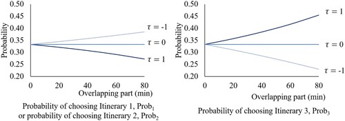
If passengers are indifferent to overlapping itineraries, the scale parameter is infinitely close to zero, that is, $\tau \to$ 0, and the scaled MISW model yields the same likelihoods as those yielded by the MNL and MNW models: $\underset{\tau \to 0}{\text{lim}}\text{ Pro}{\text{b}}_{\text{1}}=\text{Pro}{\text{b}}_{\text{2}}=\text{Pro}{\text{b}}_{\text{3}}=\frac{{100}^{-3.7}}{{100}^{-3.7}+{100}^{-3.7}+{100}^{-3.7}}=\frac{1}{3}$

If passengers dislike overlapping itineraries, the scaled MISW model sets τ to a positive value (e.g. 1) and reduces the probabilities of selecting overlapping itineraries as the extent of overlap increases. Conversely, if passengers prefer overlapping itineraries, the MISW model sets τ to a negative value (e.g. −1) and increases the probabilities of selecting overlapping itineraries as the extent of overlap increases. Hence, the scaled MISW model can resolve the problem of overlapping itineraries.

Furthermore, the heterogeneity of passengers’ perceptions is analyzed using the modified three-itinerary problem. $t_{\text{OL}}$ is set to 60 min; $\tau$ to 1; and ticket fees of the three itineraries are set to 50, 50, and 80 yuan, respectively, in the disutility function. The coefficient of fees follows a normal distribution. Its mean is fixed at 2 min/yuan, and its variance increases from 0 to 0.8. Figure 5 shows the results.

Figure 5. Change in coefficient variance for fees and the corresponding probabilities of itinerary selection.

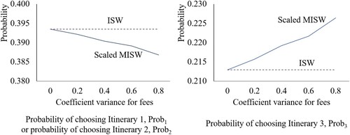
The itinerary-size weibit (ISW) model does not consider coefficient variance (i.e. ${\mathit{\sigma }}^2\to 0$ and there is no variance in $\mathit{\beta }$), so it is used for comparison with the scaled MISW model to show the effect of coefficient variance. When the coefficient variance for fees is zero, both models yield the same result. However, as the variance increases, more people are likely to be insensitive to an increase in fees and will select itineraries with higher fees. As presented in Figure 5, the rising variance does not affect the results of the ISW model but increases the $\text{Pro}{\text{b}}_{\text{3}}$ value given by the scaled MISW model. This example shows that the variance in passengers’ perceptions can be estimated using the scaled MISW model with the inclusion of random coefficients.

4. Case study

Calibration of the scaled MISW model using real-world data is presented in this section, along with a comparative analysis of the scaled MISW model with the four itinerary-choice models (i.e. the zero, MNL, MNW, and MISW models).

4.1. Data

4.1.1. Data sources

The ticket-booking data were provided by the Passenger Transport Department of the China Railway Corporation, which is responsible for the operation of all HSR trains in China. The data were collected from the HSR trains operating in the South China HSR network on 4 December 2017 (Monday). To the best of our knowledge, this was the first instance of the creation of a revealed-preference dataset for analyzing the HSR itinerary choices of passengers on the South China network and the first application of discrete-choice models for analyzing the China HSR network.

To prevent ticket scalping, Chinese railway operators require that passengers present a valid ID (e.g. Chinese resident identity card or passport) to book train tickets and enter train stations. Therefore, the railway operator can obtain some basic passenger information from these IDs, such as age and gender. Other identifying aspects of passengers’ IDs were recoded to protect their identities before the ticket-booking data were sent to us for analysis. In addition to age, gender, and recoded passenger-identification data, the ticket-booking dataset included data on time of booking, origin station, destination station, train departure and arrival times, and fare. The analyzed ticket-booking data were for the economy class, and the tickets were purchased by individuals older than 16 years of age, which meant that they could plan their own journeys. We chose ten origin–destination (OD) pairs with the highest potential for interchanges from the dataset. The basic information of these ten OD pairs is presented in Figure 6.

Figure 6. Basic information of analyzed OD pairs.

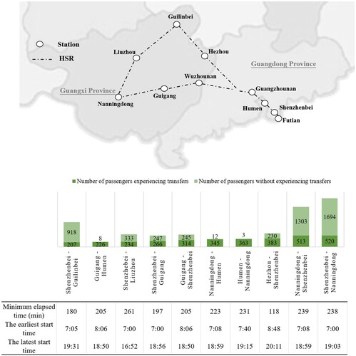
Nanningdong station is in Nanning, the capital city of Guangxi province, and Shenzhenbei station is in Shenzhen, one of the four major metropolises in China. However, only six direct high-speed trains connected these stations on the day of analysis (three in each direction). Thus, to fulfill their journey requirements (such as arriving before a certain time), passengers needed to transfer at other stations, such as Futian, Guangzhounan, Guigang, or Wuzhounan. Guangzhounan station is in Guangzhou, the capital city of Guangdong province, which has an extensive HSR network. Hence, most transfers occurred at Guangzhounan station. The situation was similar for other selected OD pairs.

China’s HSR allows passengers to book train tickets 29 days before the day on which a train departs. Thus, passengers planning a trip on 4 December 2017 could book their tickets from 5 November 2017 onwards. We set the 1st day of the booking period as the day when the ticketing was open, the 29th day as the day before the departure day, and the 30th day as the departure day. The distribution of bookings for the ten selected OD pairs during this booking period is shown in Figure 7.

Figure 7. Number of passengers booking tickets per day during the booking period.

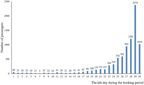
As shown in Figure 7, only a few bookings were made in the early days of the booking period. The number of bookings peaked on the day before the actual departure day, and the number of bookings on the departure day itself was the second-highest. Because the ticket fare was fixed and 4 December 2017 was not a public holiday, we assumed that a sufficient number of train tickets were available throughout the booking period. However, on the departure day, a few passengers were unable to select their most preferred itineraries,¹ and the basic assumption of adequate tickets for passengers is violated on the 30th day, as mentioned before, and the itinerary-choice models that did not consider insufficient tickets failed to simulate the passengers’ itinerary choices on the departure day. Therefore, bookings made on the 30th day were excluded from the model calibration. The total sample size in this study was 7345.

4.1.2. Construction of choice sets

According to Lurkin et al. (2017), there are two main methods for generating choice sets. The first method generates itineraries based on train timetables and several constraints, such as minimum and maximum transfer time, whereas the second method assumes that the set of observed itineraries is available to all passengers and uses it as the choice set. Because the first method often generates a choice set that includes itineraries with little to no bookings over the data-collection period, the second method is more widely used. Although the second method can be prone to bias, this problem can be mitigated if a larger dataset is used. Considering the size of our dataset, the second method was used to generate the universal choice set for an entire day. For example, five itineraries are selected by the passengers of an OD demand in the dataset, whose respective itinerary starting times are shown in Table 2.

Table 2. Five itineraries for an OD demand.

Itinerary	1	2	3	4	5
Itinerary starting time	8:30	9:30	14:30	15:30	16:30

These five itineraries are considered as five possible choices that form the universal choice set, which can be further divided according to the itinerary starting time given that the passengers might have had preferred departure times. For example, the passengers might prefer itineraries commencing early in the morning and reject those commencing in the afternoon. Hence, we divide the entire day into 12 two-hour time periods. For each OD pair, itineraries are allocated to these time periods depending on the corresponding train departure times, and the itinerary choice sets are formed for these time periods. We combine a time period with a neighboring time period if it only contains no more than one itinerary. In the example shown in Table 2, these five itinerary choices are assigned to three choice sets according to the itinerary starting time, as shown in the second column of Table 3.

Table 3. Choice sets.

Time period	Itinerary choices	Choice sets before the combination	Choice sets after the combination
[0,2)	–	i	I
[2,4)	–	ii
[4,6)	–	iii
[6,8)	–	iv
[8,10)	1,2	v
[10,12)	–	vi	II
[12,14)	–	vii
[14,16)	3,4	viii
[16,18)	5	ix
[18,20)	–	x
[20,22)	–	xi
[22,24)	–	xii

However, some time periods include no more than one itinerary choice and thus are combined with the neighboring time periods. The combination result is shown in the fourth column of Table 3. Thus, this example has two choice sets, I and II, with two and three choices, respectively. For a passenger who selects itinerary 3, his/her travel choice set is II, which includes itineraries 3–5. For the analyzed passengers, the choice set varied according to the individual, and its size ranged from 2 to 35 choices in a set.

4.1.3. Passenger characteristics

Two socio-demographics (age and gender) were included in the data. The influence of age on the booking-day pattern was analyzed (as shown in Figure 8).

Figure 8. Distribution of ticket booking during the booking period (age).

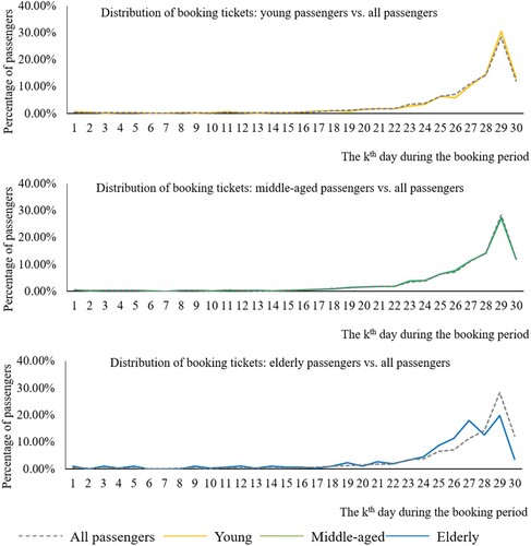
The gray dashed line in Figure 8 shows the ticket-booking pattern of all passengers. The passengers were divided into three groups: those of ages less than 31 years were included in the young group (yellow line); those of ages more than 60 years were included in the elderly group (blue line); and the rest were included in the middle-aged group (green line). The patterns of the young and middle-aged groups look similar, although more young passengers preferred to postpone the booking day than middle-aged passengers. The elderly group presented a different pattern, with a peak on the 27th day, possibly because of the small sample size of 307 individuals, compared with 3433 and 4624 individuals in the young and middle-aged groups, respectively. Alternatively, elderly passengers might have preferred to plan their journeys ahead, while the young and middle-aged passengers did not.

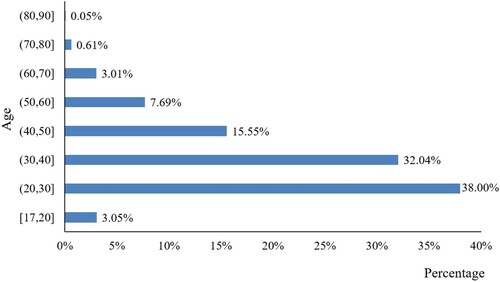
The oldest passengers in this sample was 89 years of age. In comparison, the mean age of the passengers was approximately 35.32 years. The age distribution of all of the passengers is shown in Figure 9, and most passengers are between 20 and 40 years of age, which is consistent with the literature that most HSR passengers are young (Zhen, Cao, and Tang 2019).

Figure 9. Age distributions of passengers in Datasets 1 and 2.

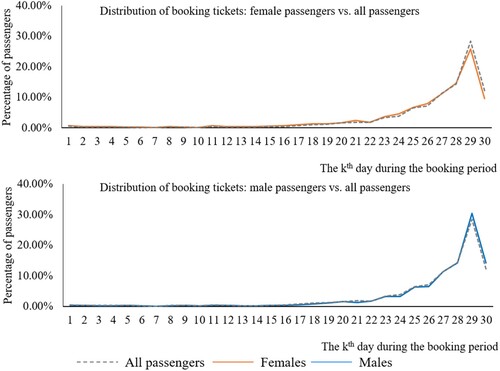
The comparison of bookings by passengers’ genders is shown in Figure 10. There was no significant difference in terms of selected booking day between female and male passengers, although female passengers appeared to be slightly more likely to book their tickets earlier. Thus, the comparison illustrated that the passengers’ gender most likely did not affect the booking-day pattern. Moreover, male passengers accounted for 56.77% of the passengers in the sample. This pattern is consistent with the finding that most HSR passengers are male (Zhen, Cao, and Tang 2019).

Figure 10. Distribution of bookings during the booking period (gender).

Moreover, the data contained information regarding the booking time, which was accurate to the second, and it is highly likely that passengers who booked tickets on the same train to travel between the same OD at the same time would travel together. Therefore, we identified whether a passenger traveled alone or in a group by checking whether the ticket booking parameters (booking time, train, and OD) were the same as those used by other passengers. We found that 2165 passengers in the sample traveled in a group.

The itinerary-choice models considered four passenger characteristics. Age is denoted as a positive real variable $y^{\text{A}}\in \mathit{y}$ that followed a normal distribution $\mathcal{N}({\overline{y}}^{\text{A}}\text{, }{\sigma }^2)$ when building the MISW and scaled MISW models. Gender is presented as a binary variable as follows: $y^{\text{M}}\text{ = }\{\begin{array}{c}\text{1, if passenger is male}\\ \text{0, if passenger is female}\end{array},y^{\text{M}}\in \mathit{y}$

In addition, whether the passenger travels in a group or alone can be presented as the following binary variable: $y^{\text{TG}}\text{ = }\{\begin{array}{c}\text{1, if passenger travels in a group}\\ \text{0, if passenger travels alone}\end{array},y^{\text{TG}}\in \mathit{y}$

The booking day is denoted as a positive integer variable $y^{\text{B}}\in \mathit{y}$ whose value ranges from 1 to 29.

4.1.4. Itinerary features

The present research (Adler, Falzarano, and Spitz 2005; Bekhor and Freund-Feinstein 2006; Collins, Rose, and Hess 2012; Lurkin et al. 2017; Ilbeigi, Lurkin, and Garrow 2019) generally considers the following itinerary attributes: (a) type of operators, (b) type of vehicles, (c) type of seats, (d) fare, (e) elapsed time, (f) in-vehicle time, (g) wait time, and (h) number of transfers. In China, there is only one HSR operator (i.e. the Passenger Transport Department of the China Railway Corporation), and the passengers are not aware of the type of vehicles when booking their tickets. Hence, the types of operators and vehicles were not included in the analyzed models. Besides, the analyzed passengers selected the same type of seats (economy class), and thus, this variable was not considered in the dataset. In contrast, the elapsed time, fare, and number of transfers were included in the dataset. The elapsed time included the IVT and transfer time. However, the ticket-booking data did not provide information about the wait times at the origin station. Hence, we assumed these to be identical. This assumption is reasonable because in China, people cannot purchase tickets for an HSR train less than 30 min before the train departs; thus, people have sufficient time to choose their preferred arrival time at the origin station after booking tickets through mobile apps or the official website.

The correlation between $b^{\text{Choice}}$ (equal to 1 if the itinerary was selected, and 0 otherwise) and itinerary features (the IVT, transfer time, elapsed time, fare, and number of transfers) was evaluated. The correlation matrix of the sample is presented in Table 4. All signs of the correlations between $b^{\text{Choice}}$ and itinerary features were negative, indicating that as the value of an itinerary feature increased, its selection probability decreased.

Table 4. Correlation matrix of the sample.

Correlation matrix	$b^{\text{Choice}}$	IVT (min)	Transfer time (min)	Elapsed time (min)	Number of transfers	Fare (yuan)
$b^{\text{Choice}}$	1.00
IVT (min)	−0.10	1.00
Transfer time (min)	−0.22	0.06	1.00
Elapsed time (min)	−0.23	0.69	0.77	1.00
Number of transfers	−0.71	0.13	0.28	0.29	1.00
Fare (yuan)	−0.03	0.85	0.07	0.59	0.05	1.00

Fare is the least likely attribute to be linked to $b^{\text{Choice}}$, and is significantly correlated with IVT and elapsed time. This may be because the running speed of HSR is relatively stable, and China HSR sets ticket fares according to the running mileage.² For example, the basic price of an economy-class ticket is approximately 0.46 yuan/km. Moreover, the ticket fare and number of transfers are weakly correlated because the ticket fare of an itinerary with transfers may not be different from that of a direct itinerary. For instance, passengers traveling from Hezhou to Shenzhenbei pay the same fare (155 yuan), regardless of whether they select a direct train or take a transfer at Guangzhounan station. This correlation results in an incorrect sign for the estimated value, indicating that an itinerary with a higher fare is more likely to be selected when fare is included in the calibration models. Therefore, fare is ignored when building the disutility function. Similarly, the strong correlations between IVT, transfer time, and elapsed time suggest that these three itinerary features cannot be included in one model. Hence, to include the influences of journey time and transfers, two possible combinations were considered: (a) IVT, transfer time, and number of transfers and (b) elapsed time and number of transfers. Because elapsed time is more likely than the transfer time and IVT to be related to $b^{\text{Choice}}$, we adopted the second combination for further analysis.

The disutility function comprised two types of features for itinerary $i$: elapsed time ($x_i^{\text{ElapsedTime}}$, unit: min) and number of transfers ($x_i^{\text{TransferNumber}}$). The respective coefficients ${\beta }^{\text{ElapsedTime}}$ and ${\beta }^{\text{TransferNumber}}$ were defined as follows (Equations (12) and (13)): (12) ${\beta }^{\text{ElapsedTime}}={\theta }^{\text{E}-\text{A}}{y}^{\text{A}}+{\theta }^{\text{E}-\text{M}}{y}^{\text{M}}+{\theta }^{\text{E}-\text{TG}}{y}^{\text{TG}}+{\theta }^{\text{E}-\text{B}}{y}^{\text{B}}+{\tilde{\theta }}^{\text{E}}$(12) and (13) ${\beta }^{\text{TransferNumber}}={\theta }^{\text{T}-\text{A}}{y}^{\text{A}}+{\theta }^{\text{T}-\text{M}}{y}^{\text{M}}+{\theta }^{\text{T}-\text{TG}}{y}^{\text{TG}}+{\theta }^{\text{T}-\text{B}}{y}^{\text{B}}+{\tilde{\theta }}^{\text{T}}$(13) where ${\theta }^{\text{E}-\text{A}}$ and ${\theta }^{\text{T}-\text{A}}$ reflect the effect of passenger age on these two coefficients; ${\theta }^{\text{E}-\text{M}}$ and ${\theta }^{\text{T}-\text{M}}$ reflect this effect in case of a male passenger; ${\theta }^{\text{E}-\text{TG}}$ and ${\theta }^{\text{T}-\text{TG}}$ reflect this effect for group travel; ${\theta }^{\text{E}-\text{B}}$ and ${\theta }^{\text{T}-\text{B}}$ reflect the effect of booking day on these two coefficients; and ${\tilde{\theta }}^{\text{E}}$ and ${\tilde{\theta }}^{\text{T}}$ are constants.

4.2. Model specification

We assumed that itinerary-choice models provided the same set of estimated variables for the analyzed OD pairs. Based on the above description of passenger characteristics and itinerary features, the scaled MISW model was built for calibration, and its disutility function specification with 14 estimated variables was as follows (Equation (14)): (14) ${\check{U}}_i=\frac{{({\beta }^{\text{ElapsedTime}}{x}_i^{\text{ElapsedTime}}+{\beta }^{\text{TransferNumber}}{x}_i^{\text{TransferNumber}}-\xi )}^{\gamma }}{{({\omega }_i)}^{\tau }},\mathrm{\forall }i\in \mathit{I}$(14)

Four other itinerary-choice models were created for comparison with the scaled MISW model.

1. The zero model assumes that the socio-demographic and itinerary features do not affect passengers’ itinerary choices and passengers are distributed equally across all of the available itineraries. Hence, it has zero estimated variables.

2. The disutility function of the MNL model was specified as follows (Equation (15)): (15) ${\stackrel{⌣}{U}}_i={\beta }^{\text{ElapsedTime}}{x}_i^{\text{ElapsedTime}}+{\beta }^{\text{TransferNumber}}{x}_i^{\text{TransferNumber}},\mathrm{\forall }i\in \mathit{I}$(15) Therefore, the MNL model has 10 estimated variables.

3. The disutility function of the MNW model was specified as follows (Equation (16)): (16) ${\stackrel{⌣}{U}}_i=({\beta }^{\text{ElapsedTime}}{x}_i^{\text{ElapsedTime}}+{\beta }^{\text{TransferNumber}}{x}_i^{\text{TransferNumber}}-\xi {)}^{\gamma },\mathrm{\forall }i\in \mathit{I}$(16) Hence, the MNW model has 12 estimated variables.

4. The disutility function of the MISW was specified as follows (Equation (17)): (17) ${\stackrel{⌣}{U}}_i=\frac{{({\beta }^{\text{ElapsedTime}}{x}_i^{\text{ElapsedTime}}+{\beta }^{\text{TransferNumber}}{x}_i^{\text{TransferNumber}}-\xi )}^{\gamma }}{{\omega }_i},\mathrm{\forall }i\in \mathit{I}$(17) Thus, it has 13 estimated variables.

4.3. Results

The simulated maximum likelihood estimation method was used to evaluate the integrals, and the model calibration was performed in the R software environment (R Core Team 2018) by using two packages: ‘bbmle’ (Bolker 2017) and ‘dplyr’ (Wickham et al. 2019). The ‘bbmle’ package offers the mle2 function to estimate the model parameters, and we used the default setting of this function, in which the mle2 function runs the Broyden–Fletcher–Goldfarb–Shanno (BFGS) algorithm (Broyden 1970; Fletcher 1970; Goldfarb 1970; Shanno 1970), which is a quasi-Newton method and exhibits satisfactory performance for optimization problems.

The estimation result of the scaled MISW model is given in Table 5, and a comparison of the results obtained using the scaled MISW model with those obtained using the other four models is presented in Table 6. The discussion of these two tables is given in Section 5.

Table 5. Estimation results of the scaled MISW model.

Estimated variables	Estimated value	z value
Location parameter $\xi$	0.001	0.001
Shape parameter $\gamma$	5.483	25.575
Standard deviation of age $\sigma$	5.762	97.193
Factors related to elapsed time:
Male ${\theta }^{\text{E}-\text{M}}$	0.023	2.100
Age ${\theta }^{\text{E}-\text{A}}$	0.003	5.420
Travel in a group ${\theta }^{\text{E}-\text{TG}}$	0.017	1.437
Booking day ${\theta }^{\text{E}-\text{B}}$	0.009	8.732
Constant ${\tilde{\theta }}^{\text{E}}$	−0.017	−0.864
Factors related to number of transfers:
Male ${\theta }^{\text{T}-\text{M}}$	0.479	13.476
Age ${\theta }^{\text{T}-\text{A}}$	1.311	7.270
Travel in a group ${\theta }^{\text{T}-\text{TG}}$	−0.167	−1.442
Booking day ${\theta }^{\text{T}-\text{B}}$	1.602	4.191
Constant ${\tilde{\theta }}^{\text{T}}$	0.407	4.875
Scale factor $\tau$	−0.300	−4.873

Table 6. Log-likelihood and overall goodness-of-fit measures of itinerary-choice models.

Model	Number of estimated variables	Log-likelihood	AIC	BIC	Rho-squared	Adjusted rho-squared
zero	0	−18,079	36,157	36,157	–	–
MNL	10	−9772	19,563	19,632	0.459	0.459
MNW	12	−8427	16,877	16,960	0.534	0.533
MISW	13	−8775	17,576	17,666	0.515	0.514
Scaled MISW	14	−8402	16,832	16,928	0.535	0.534

5. Discussion

We discuss the comparison results in Section 5.1, and then interpret the estimation results of the scaled MISW model in Section 5.2.

5.1. Model performance

For comparison, we calculated the log-likelihood and the overall goodness-of-fit measures, namely the Akaike information criterion (AIC) (Akaike 1974), Bayesian information criterion (BIC) (Schwarz 1978), rho-squared value, and adjusted rho-squared value (Garrow 2010). The rho-squared and adjusted rho-squared values were calculated with respect to the zero model.

The likelihood that the passenger loading was uniform was the lowest in the zero model, which had the smallest log-likelihood and the largest AIC and BIC values. The other four models yielded significantly better estimation results than the zero model, as indicated by the notable distinctions in their log-likelihood and overall goodness-of-fit measures. Thus, the passengers’ decisions were influenced by their characteristics and itinerary features.

The weibit-type models (MNW, MISW, and scaled MISW models) performed better than the MNL model. For example, the AIC and BIC values of the MNW model were approximately 2500 less than those of the MNL model, and its rho-squared and adjusted rho-squared values were greater than those of the MNL model by approximately 16.2%. These results indicate that the weibit-type models make more reasonable assumptions regarding the distribution of the random-error term than the MNL model when the passengers’ trip lengths are considerably different. The minimum elapsed time for the 10 analyzed OD pairs ranged from 118 to 261 min. These values are similar to those shown in the two-itinerary example presented in Section 3.3, and the empirical result might have been consistent with the numerical analysis results. The MNL model could not handle the length-specific perception variance, whereas the weibit-type models could handle it.

Due to the inclusion of the scaled IS factor and the standard deviation of age, the scaled MISW model performed the best because its overall goodness-of-fit measures were better than those of the weibit-type models. In addition, the MNW model performed better than the MISW model, indicating that an incorrect assumption of the passengers’ perception regarding the overlapping itinerary could result in a worse calibration result than that obtained by the model that did not consider the overlap. Hence, the worst performance exhibited by the MISW model indicated the need to set a scale parameter for the IS factor to reflect the passengers’ perceptions of overlapping itineraries.

5.2. Model results

5.2.1. Interpretation of results

As indicated by the estimation results, the calibrated scaled MISW disutility (Equation (14)) is a function of $\gamma \text{ = }$5.483 and $\xi \text{ = }$0.001. All estimated variables were highly significant, except for $\xi$, ${\tilde{\theta }}^{\text{E}}$, ${\theta }^{\text{E}-\text{TG}}$, and ${\theta }^{\text{T}-\text{TG}}$.

The standard deviation of age ($\sigma$) is a continuous variable that represents the level of heterogeneity among passengers of the same age. The scaled MISW model estimated $\sigma$ as 5.762 and its respective z value as approximately 97.193. This indicates that peers (i.e. people of the same age) were likely heterogeneous.

The variable influence on elapsed time if passenger is male (${\theta }^{\text{E}-\text{M}}$) had a positive sign, which indicated that male passengers were more sensitive to elapsed time than female passengers, possibly because of the gender difference in income. Qu, Guo, and Wang (2019) revealed that, generally, males earn more than females in China. Compared to a person with a lower income, a person with a higher income values their time more and may have more options (such as airplanes) to complete their trips and avoid a long travel time if they are not satisfied with the HSR itinerary choices. This gender difference can also assign a positive sign to the variable influence on number of transfers if passenger is male (${\theta }^{\text{T}-\text{M}}$), which indicates that male travelers evaluate a transfer more negatively than female travelers, possibly because a transfer generally requires extra waiting time at stations.

The variable age effect on elapsed time (${\theta }^{\text{E}-\text{A}}$) had a positive sign, which indicates that elderly passengers view the increased elapsed time less favorably than younger passengers. This result appears consistent with some previous findings: elderly people consider long rides uncomfortable (Batra 2009) and tire more easily because they have less physical strength than younger passengers (Szeto et al. 2017). Hence, they tend to travel for shorter periods, as compared to younger passengers (Liu et al. 2017; Szeto et al. 2017; Shrestha et al. 2017). Moreover, older passengers are more likely to have a higher income and higher position, and thus, may prefer to spend their time on other activities with a higher utility than traveling by train and would tend to select the option that offers the shortest travel time.

The variable age effect on number of transfers (${\theta }^{\text{T}-\text{A}}$) had a positive sign, suggesting that younger passengers are more likely to tolerate transfers than elderly passengers. This finding is consistent with results obtained by Szeto et al. (2017). Besides the income difference, another reason is that younger passengers are physically stronger than elderly passengers (Janssen et al. 2000; Shrestha et al. 2017) and thus can better cope with the extra walking/climbing, as a transfer mostly involves a long queue to access elevators or climbing stairs.

The variables influence on elapsed time if passenger travels in a group (${\theta }^{\text{E}-\text{TG}}$) and influence on number of transfers if passenger travels in a group (${\theta }^{\text{T}-\text{TG}}$) had low z values, indicating that the values of ${\theta }^{\text{E}-\text{TG}}$ and ${\theta }^{\text{T}-\text{TG}}$ did not statistically significantly differ from zero. Apparently, the influence of whether traveling with others on itinerary choices was not significant for the analyzed passengers. However, the travel group behavior is an interesting study topic that can influence passenger behavior in other aspects as well, for example, selecting HSR or air trips. Hence, it is worth studying in the future.

The variables booking day effect on elapsed time (${\theta }^{\text{E}-\text{B}}$) and booking day effect on number of transfers (${\theta }^{\text{T}-\text{B}}$) had a positive sign, which indicates that passengers who book tickets at a later stage assess the increased elapsed time and number of transfers as more unpleasurable than those who book the tickets earlier. When the travel plan is certain, passengers will book their tickets, and good knowledge about the travel plan may help relieve some travel anxiety caused by the uncertainty about the arrival at the destination. More likely, passengers who book tickets at an earlier stage have advanced and better knowledge about the travel plan than those who book tickets at a later stage (especially on the days near the departure day). Thus, the latter might have more travel anxiety and would be more likely to avoid itineraries with longer elapsed time or more transfers, which would increase the risk of missing the selected trains.

The variable scale parameter ($\tau$) had a negative sign, indicating that the passengers were optimistic about overlapping itineraries. The overlapping part of an HSR itinerary is generally an HSR route that connects two major terminals. This HSR route tends to be served by vehicles with larger capacities and better services (e.g. diversified meal choices) than average, meaning that the passengers can have a more comfortable travel experience. In addition, there are likely to be more alternative trains because a connection between two major terminals is likely to have a higher-than-average frequency of service. Therefore, if passengers miss their selected HSR trains, they can easily find an alternative. This result agrees with those obtained by Hoogendoorn-Lanser and Bovy (2007) and Anderson, Nielsen, and Prato (2017).

5.2.2. Temporal value of number of transfers

The above discussion of the correlation between $b^{\text{Choice}}$ suggests that the scaled MISW model should have positive coefficients ${\beta }^{\text{ElapsedTime}}$ and ${\beta }^{\text{TransferNumber}}$. The expected ${\beta }^{\text{ElapsedTime}}$ and ${\beta }^{\text{TransferNumber}}$ were calculated using Equations (12) and (13), and they had a positive sign for all of the passengers. Furthermore, the ratio between the expected ${\beta }^{\text{TransferNumber}}$ and ${\beta }^{\text{ElapsedTime}}$ was used to analyze and understand choice behavior. This ratio was denoted as the temporal value of the number of transfers (TVofNT) and calculated as follows (Equation (18)): (18) $\text{Temporal value of number of transfers}=\frac{{\beta }^{\text{TransferNumber}}}{{\beta }^{\text{ElapsedTime}}}$(18)

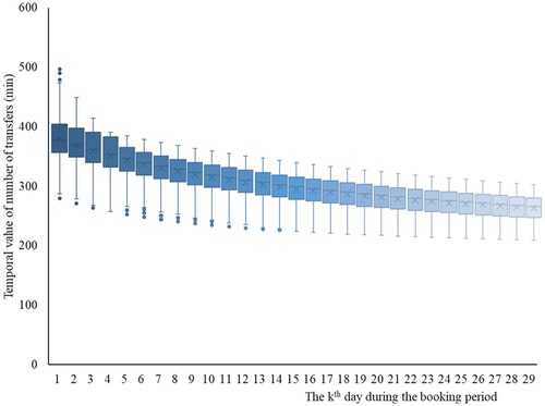
The TVofNT variable measures how much elapsed time a passenger can bear to avoid a transfer. The value range of TVofNT changes with booking day, as depicted in Figure 11. As indicated by the positive signs of variables ${\theta }^{\text{E}-\text{B}}$ and ${\theta }^{\text{T}-\text{B}}$, the disutility of the elapsed time and number of transfers increased when the booking day was closer to the departure day, and the trend in the disutility of the elapsed time seemed to increase faster than that of the number of transfers, as shown in Figure 11, where the TVofNT for passengers who booked tickets at a later stage was less than that for passengers who booked tickets earlier. The passengers who booked tickets at a later stage appeared to have an urgent need to travel, and might have had a greater requirement for the journey time. In addition, the TVofNT for passengers who booked tickets later varied less than that for passengers who booked tickets earlier. This finding supports the contention that passengers who book tickets near the departure day exhibit more uniform choice behaviors (Hetrakul and Cirillo 2013).

Figure 11. Temporal value of number of transfers.

Another difference in the TVofNT variable was related to gender. Male passengers had a lower TVofNT than female passengers when the other conditions (i.e. age, booking day, and whether traveling in group or alone) were the same. This difference indicated that male passengers preferred to spend less elapsed time to avoid a transfer than female passengers because males generally have a higher income level and might place a greater value on their time.

Besides these differences, for elderly passengers, the trend of the disutility of the number of transfers seemed to increase faster than that of the elapsed time. Thus, the TVofNT for elderly passengers tended to be higher than that for younger passengers when the other conditions (i.e. gender, booking day, and whether traveling alone or in a group) were the same. This result indicates that elderly passengers prefer spending more elapsed time to avoid a transfer than younger passengers. Possibly the physical inability to cope with transfers has a non-negligible impact on the preference of passengers.

The existing HSR itinerary-choice models (Sun et al. 2018) do not simultaneously analyze the elapsed time and number of transfers, but a few airline itinerary-choice models have considered these two itinerary features. Thus, the TVofNT was calculated using these models as a reference in this study. Table 7 presents the TVofNTs computed in a few previous studies of airline systems.

Table 7. TVofNTs computed in previous studies on airlines.

Research	Studied time	Country	TVofNT (min)
Adler, Falzarano, and Spitz (2005)	2000	US	30.23–41.68
Collins, Rose, and Hess (2012)	2008	Australia	276.36
Lurkin et al. (2017)	2013	US	466.22–511.64
Ilbeigi, Lurkin, and Garrow (2019)	2016–2017	US	343.05–419.26

As inferred from Table 7, the range of TVofNT for airlines is 30.23–511.64 min. The TVofNT values in this study ranged within [206.66, 493.44]. Thus, the TVofNTs obtained in this study were within the range of those obtained in the studies of airlines. Moreover, the TVofNT values obtained in this study were lower than the highest value presented in Table 7, especially those of passengers who booked tickets after the 3rd booking day, which were less than 400. There are two possible reasons for this.

1. Transfers in the HSR system are simpler than those in an airline system. A transfer in an airline system may involve clearing customs, collecting baggage, and check-in for the next flight to obtain the next boarding pass, whereas HSR passengers in our datasets traveled within the same country, so they did not need to clear customs, and they could take their baggage with them onboard.

2. The punctuality of the HSR system is greater than that of airlines, so the HSR passengers would have had fewer concerns about missing their connection than airline passengers.

6. Conclusions

In this paper, four itinerary-choice models were applied to the ticket-booking data for 10 OD pairs in the South China HSR network. The log-likelihood and overall goodness-of-fit measures illustrated that the scaled MISW model best suited the data, and that the MNW model provided a better estimation result than the MNL model. In addition, the results supported the need to consider random preference variations among passengers and the scale parameter for the IS factor, which would reflect the passengers’ perceptions of the itinerary overlap. Hence, this case study provided evidence for the superiority of the scaled MISW model in estimating route-choice behaviors in a schedule-based railway system. Furthermore, the calibration results showed that the age, gender, and booking day influenced the HSR itinerary choices. However, this study has several limitations that need to be addressed in future studies:

1. Age was assumed to follow the commonly used normal distribution. However, it may follow another distribution, in which case the assumption of normal distribution would affect the estimation performance. Thus, the future calibration practice should explore the possible age distributions.

2. Because of the difficulty faced in data collection, the present study focuses on a relatively simple network. Theoretically, the scaled MISW model can handle a large number of choices and more complex networks. However, it requires a longer computation time than the MNL and MNW models because of the IS factor and integration calculations. The long computation time may not be a huge issue for an offline problem, but it may be a concern for online or real-time problems. Hence, in the future, the possible practical applications of the scaled MISW model should be analyzed according to the problem setting.

3. Because of the limited data availability, the desired departure and arrival times, which have a negligible influence on passengers’ itinerary choices, were not included in the proposed choice models. In the future, we will attempt to collect these data through the stated preference surveys and analyze the influence of these times on HSR itinerary choices.

4. The scaled MISW model has further scope for improvement. For example, the extended PSW model considers elastic demand (Kitthamkesorn, Chen, and Xu 2015); however, the scaled MISW model assumes only fixed demand. Thus, future studies can extend this model to consider elastic demand.

5. More tests using real-world data, including additional passenger characteristics, should be conducted to verify the feasibility of weibit-type models. One possible testing approach is to apply these models to a service network and compare the estimated onboard passenger flows with the real flows. In the future, we will collect more data and work further on this test.

Data availability statement

The data that support the findings of this study were provided by the Passenger Transport Department of the China Railway Corporation. Restrictions apply to the availability of these data, which were used under license for this study.

Disclosure statement

No potential conflict of interest was reported by the author(s).

Additional information

Funding

The work described in this paper was supported by a grant from the Research Grants Council of the Hong Kong Special Administrative Region, China [Project No. [T32-101/15-R]]. The second author is supported by two scholarships (a Postgraduate Scholarship from the University of Hong Kong and a University Postgraduate Fellowship from the Jessie and George Ho Charitable Foundation). The third author is supported by research grants from the Research Grants Council of the Hong Kong Special Administrative Region [Project No. 15212217] and the Research Committee of the Hong Kong Polytechnic University [Project No. 1-ZVJV]. The fourth author is supported by the Francis S Y Bong Endowed Professorship in Engineering. The fifth author is supported by the Hong Kong Scholars Program 2017 and the National Natural Science Foundation of China [No. 71701174].

Notes

1 There are two possible reasons for this: first, there might have been insufficient tickets following the large number of bookings on the 29th day; second, there might have been fewer feasible itineraries, because some trains had already departed.

2 China railway passenger tickets and fares: https://zh.wikipedia.org/wiki/%E4%B8%AD%E5%9B%BD%E9%93%81%E8%B7%AF%E5%AE%A2%E8%BF%90%E8%BD%A6%E7%A5%A8%E4%B8%8E%E7%A5%A8%E4%BB%B7#cite_note-70 (Accessed 24 April 2020).

References

- Adler, Thomas, C. Stacey Falzarano, and Gregory Spitz. 2005. “Modeling Service Trade-Offs in Air Itinerary Choices.” Transportation Research Record: Journal of the Transportation Research Board 1915: 20–26. doi:10.1177/0361198105191500103.
- Akaike, Hirotugu. 1974. “A new Look at the Statistical Model Identification.” IEEE Transactions on Automatic Control 19 (6): 716–723. doi:10.1109/TAC.1974.1100705.
- Anderson, Marie Karen, Otto Anker Nielsen, and Carlo Giacomo Prato. 2017. “Multimodal Route Choice Models of Public Transport Passengers in the Greater Copenhagen Area.” EURO Journal on Transportation and Logistics 6 (3): 221–245. doi:10.1007/s13676-014-0063-3.
- Batra, Adarsh. 2009. “Senior Pleasure Tourists: Examination of Their Demography, Travel Experience, and Travel Behavior upon Visiting the Bangkok Metropolis.” International Journal of Hospitality & Tourism Administration 10 (3): 197–212. doi:10.1080/15256480903088105.
- Bekhor, Shlomo, and Uzi Freund-Feinstein. 2006. “Modeling Passengers’ Preferences on a Short-Haul Domestic Airline with Rank-Ordered Data.” Transportation Research Record: Journal of the Transportation Research Board 1951: 1–6. doi:10.1177/0361198106195100101.
- Ben-Akiva, Moshe, and Michel Bierlaire. 1999. “Discrete Choice Methods and Their Applications to Short Term Travel Decisions.” In Handbook of Transportation Science, edited by Randolph Hall, 5–33. Boston, MA: Springer.
- Bolker, Ben, and R Development Core Team. 2017. bbmle: Tools for General Maximum Likelihood Estimation. R Package Version 1.0.20. R Foundation for Statistical Computing. https://CRAN.R-project.org/package=bbmle.
- Broyden, C. G. 1970. “The Convergence of a Class of Double-Rank Minimization Algorithms.” Journal of Applied Mathematics 6 (1): 76–90. doi:10.1093/imamat/6.1.76.
- Cacchiani, Valentina, Jianguo Qi, and Lixing Yang. 2020. “Robust Optimization Models for Integrated Train Stop Planning and Timetabling with Passenger Demand Uncertainty.” Transportation Research Part B: Methodological 136: 1–29. doi:10.1016/j.trb.2020.03.009.
- Cascetta, Ennio, Agostino Nuzzolo, Francesco Russo, and Antonino Vitetta. 1996. “A Modified Logit Route Choice Model Overcoming Path Overlapping Problems Specification and Some Calibration Results for Interurban Networks.” Paper Presented at the ISTTT Conference, Lyon, France.
- Castillo, Enrique, José María Menéndez, Pilar Jiménez, and Ana Rivas. 2008. “Closed Form Expressions for Choice Probabilities in the Weibull Case.” Transportation Research Part B: Methodological 42 (4): 373–380. doi:10.1016/j.trb.2007.08.002.
- Chen, Anthony, Surachet Pravinvongvuth, Xiangdong Xu, Seungkyu Ryu, and Piya Chootinan. 2012. “Examining the Scaling Effect and Overlapping Problem in Logit-Based Stochastic User Equilibrium Models.” Transportation Research Part A: Policy and Practice 46 (8): 1343–1358. doi:10.1016/j.tra.2012.04.003.
- Chou, Pin-Fenn, Chin-Shan Lu, and Yu-Hern Chang. 2014. “Effects of Service Quality and Customer Satisfaction on Customer Loyalty in High-Speed Rail Services in Taiwan.” Transportmetrica A: Transport Science 10 (10): 917–945. doi:10.1080/23249935.2014.915247.
- Collins, Andrew, John Rose, and Stephane Hess. 2012. “Interactive Stated Choice Surveys: A Study of Air Travel Behaviour.” Transportation 39 (1): 55–79. doi:10.1007/s11116-011-9327-z.
- Daganzo, Carlos F., and Yosef Sheffi. 1977. “On Stochastic Models of Traffic Assignment.” Transportation Science 11 (3): 253–274. doi:10.1287/trsc.11.3.253.
- Dial, Robert B. 1971. “A Probabilistic Multipath Traffic Assignment Model Which Obviates Path Enumeration.” Transportation Research 5 (2): 83–111. doi:10.1016/0041-1647(71)90012-8.
- Fletcher, R. 1970. “A New Approach to Variable Metric Algorithms.” The Computer Journal 13 (3): 317–322. doi:10.1093/comjnl/13.3.317.
- Fosgerau, Mogens, and Michel Bierlaire. 2009. “Discrete Choice Models with Multiplicative Error Terms.” Transportation Research Part B: Methodological 43 (5): 494–505. doi:10.1016/j.trb.2008.10.004.
- Garrow, Laurie A. 2010. Discrete Choice Modelling and Air Travel Demand: Theory and Applications. Farnham: Ashgate.
- Goldfarb, Donald. 1970. “A Family of Variable-Metric Methods Derived by Variational Means.” Mathematics of Computation 24 (109): 23–26. doi:10.1090/S0025-5718-1970-0258249-6.
- Hamdouch, Younes, W. Y. Szeto, and Y. Jiang. 2014. “A New Schedule-Based Transit Assignment Model with Travel Strategies and Supply Uncertainties.” Transportation Research Part B: Methodological 67: 35–67. doi:10.1016/j.trb.2014.05.002.
- Hess, Stephane, Tim Ryley, Lisa Davison, and Thomas Adler. 2013. “Improving the Quality of Demand Forecasts Through Cross Nested Logit: A Stated Choice Case Study of Airport, Airline and Access Mode Choice.” Transportmetrica A: Transport Science 9 (4): 358–384. doi:10.1080/18128602.2011.577758.
- Hetrakul, Pratt, and Cinzia Cirillo. 2013. “Accommodating Taste Heterogeneity in Railway Passenger Choice Models Based on Internet Booking Data.” Journal of Choice Modelling 6: 1–16. doi:10.1016/j.jocm.2013.04.003.
- Hoogendoorn-Lanser, Sascha, and Piet Bovy. 2007. “Modeling Overlap in Multimodal Route Choice by Including Trip Part-Specific Path Size Factors.” Transportation Research Record 2003 (1): 74–83. doi:10.3141/2003-10.
- Ilbeigi, Mohammad, Virginie Lurkin, and Laurie A. Garrow. 2019. “Using Internet-Based Marketplaces to Conduct Surveys: An Application to Airline Itinerary Choice Models.” Transportation Research Part C: Emerging Technologies 103: 129–141. doi:10.1016/j.trc.2019.03.025.
- Janssen, Ian, Steven B. Heymsfield, ZiMian Wang, and Robert B. Ross. 2000. “Skeletal Muscle Mass and Distribution in 468 Men and Women Aged 18–88 yr.” Journal of Applied Physiology 89 (1): 81–88. doi:10.1152/jappl.2000.89.1.81.
- Jou, Rong-Chang, Jung-Yi Chien, and Yuan-Chan Wu. 2013. “A Study of Passengers’ Willingness to Pay for Business Class Seats of High-Speed Rail in Taiwan.” Transportmetrica A: Transport Science 9 (3): 223–238. doi:10.1080/18128602.2011.565816.
- Kitthamkesorn, Songyot, and Anthony Chen. 2013. “A Path-Size Weibit Stochastic User Equilibrium Model.” Transportation Research Part B: Methodological 57: 378–397. doi:10.1016/j.trb.2013.06.001.
- Kitthamkesorn, Songyot, and Anthony Chen. 2014. “Unconstrained Weibit Stochastic User Equilibrium Model with Extensions.” Transportation Research Part B: Methodological 59: 1–21. doi:10.1016/j.trb.2013.10.010.
- Kitthamkesorn, Songyot, Anthony Chen, and Xiangdong Xu. 2015. “Elastic Demand with Weibit Stochastic User Equilibrium Flows and Application in a Motorised and Non-Motorised Network.” Transportmetrica A: Transport Science 11 (2): 158–185. doi:10.1080/23249935.2014.944241.
- Kurauchi, Fumitaka, and H. Ido. 2017. “Estimation of the Expressway/Surface Road Choice Model Using Logit-Weibit Hybrid Model.” Paper Presented at the 22nd International Conference of Hong Kong Society for Transportation Studies, Hong Kong, China.
- Li, Zhi-Chun, William H. K. Lam, S. C. Wong, and A. Sumalee. 2010. “An Activity-Based Approach for Scheduling Multimodal Transit Services.” Transportation 37 (5): 751–774. doi:10.1007/s11116-010-9291-z.
- Lim, Yongtaek, and Hyunmyung Kim. 2016. “A Combined Model of Trip Distribution and Route Choice Problem.” Transportmetrica A: Transport Science 12 (8): 721–735. doi:10.1080/23249935.2016.1166171.
- Liu, Wenzhi, Huapu Lu, Zhiyuan Sun, and Jing Liu. 2017. “Elderly’s Travel Patterns and Trends: The Empirical Analysis of Beijing.” Sustainability 9 (6): 981. doi:10.3390/su9060981.
- Lurkin, Virginie, Laurie A. Garrow, Matthew J. Higgins, Jeffrey P. Newman, and Michael Schyns. 2017. “Accounting for Price Endogeneity in Airline Itinerary Choice Models: An Application to Continental U.S. Markets.” Transportation Research Part A: Policy and Practice 100: 228–246. doi:10.1016/j.tra.2017.04.007.
- Nuzzolo, Agostino, Francesco Russo, and Umberto Crisalli. 2001. “A Doubly Dynamic Schedule-Based Assignment Model for Transit Networks.” Transportation Science 35 (3): 268–285. doi:10.1287/trsc.35.3.268.10149.
- Pimentel, Pedro, Cláudia Nunes, and Gualter Couto. 2018. “High-Speed Rail Transport Valuation with Stochastic Demand and Investment Cost.” Transportmetrica A: Transport Science 14 (4): 275–291. doi:10.1080/23249935.2017.1384936.
- Qu, Dan, Saisai Guo, and Lafang Wang. 2019. “Experience, Tenure and Gender Wage Difference: Evidence from China.” Economic Research-Ekonomska Istraživanja 32 (1): 1169–1184. doi:10.1080/1331677X.2019.1592695.
- R Core Team. 2018. R: A Language and Environment for Statistical Computing. Vienna: R Foundation for Statistical Computing. https://www.R-project.org/.
- Schwarz, Gideon. 1978. “Estimating the Dimension of a Model.” Annals of Statistics 6 (2): 461–464. doi:10.1214/aos/1176344136.
- Shanno, David F. 1970. “Conditioning of Quasi-Newton Methods for Function Minimization.” Mathematics of Computation 24 (111): 647–656. doi:10.1090/S0025-5718-1970-0274029-X.
- Sheffi, Yosef. 1985. Urban Transportation Networks: Equilibrium Analysis with Mathematical Programming Methods. Englewood Cliffs, NJ: Prentice-Hall.
- Shrestha, B. P., A. Millonig, N. B. Hounsell, and M. McDonald. 2017. “Review of Public Transport Needs of Older People in European Context.” Journal of Population Ageing 10 (4): 343–361. doi:10.1007/s12062-016-9168-9.
- Sun, Yanshuo, Zhibin Jiang, Jinjing Gu, Min Zhou, Yeming Li, and Lei Zhang. 2018. “Analyzing High Speed Rail Passengers’ Train Choices Based on New Online Booking Data in China.” Transportation Research Part C: Emerging Technologies 97: 96–113. doi:10.1016/j.trc.2018.10.015.
- Szeto, W. Y., Linchuan Yang, R. C. P. Wong, Y. C. Li, and S. C. Wong. 2017. “Spatio-Temporal Travel Characteristics of the Elderly in an Ageing Society.” Travel Behaviour and Society 9: 10–20. doi:10.1016/j.tbs.2017.07.005.
- Tong, C. O., and A. J. Richardson. 1984. “A Computer Model for Finding the Time-Dependent Minimum Path in a Transit System with Fixed Schedules.” Journal of Advanced Transportation 18 (2): 145–161. doi:10.1002/atr.5670180205.
- Van Nes, Rob, Sascha Hoogendoorn-Lanser, and Frank S. Koppelman. 2008. “Using Choice Sets for Estimation and Prediction in Route Choice.” Transportmetrica 4 (2): 83–96. doi:10.1080/18128600808685686.
- Wickham, Hadley, Romain François, Lionel Henry, and Kirill Müller. 2019. dplyr: A Grammar of Data Manipulation. R Package Version 0.8.0.1. R Foundation for Statistical Computing. https://CRAN.R-project.org/package=dplyr.
- Xie, J., S. C. Wong, and S. M. Lo. 2017. “Three Extensions of Tong and Richardson’s Algorithm for Finding the Optimal Path in Schedule-Based Railway Networks.” Journal of Advanced Transportation 2017: 9216864. doi:10.1155/2017/9216864.
- Xie, J., S. C. Wong, S. Zhan, S. M. Lo, and Anthony Chen. 2020. “Train Schedule Optimization Based on Schedule-Based Stochastic Passenger Assignment.” Transportation Research Part E: Logistics and Transportation Review 136: 101882. doi:10.1016/j.tre.2020.101882.
- Xie, Jiemin, Shuguang Zhan, S. C. Wong, and S. M. Lo. 2021. “A Schedule-Based Timetable Model for Congested Transit Networks.” Transportation Research Part C: Emerging Technologies 124: 102925. doi:10.1016/j.trc.2020.102925.
- Yap, Menno, Oded Cats, and Bart van Arem. 2018. “Crowding Valuation in Urban Tram and Bus Transportation Based on Smart Card Data.” Transportmetrica A: Transport Science 16 (1): 23–42. doi:10.1080/23249935.2018.1537319.
- Yilmaz, Veysel, and Erkan Ari. 2017. “The Effects of Service Quality, Image, and Customer Satisfaction on Customer Complaints and Loyalty in High-Speed Rail Service in Turkey: A Proposal of the Structural Equation Model.” Transportmetrica A: Transport Science 13 (1): 67–90. doi:10.1080/23249935.2016.1209255.
- Zhan, Shuguang, S. C. Wong, and S. M. Lo. 2020. “Social Equity-Based Timetabling and Ticket Pricing for High-Speed Railways.” Transportation Research Part A: Policy and Practice 137: 165–186. doi:10.1016/j.tra.2020.04.018.
- Zhang, Chuntian, Yuan Gao, Lixing Yang, Ziyou Gao, and Jianguo Qi. 2020. “Joint Optimization of Train Scheduling and Maintenance Planning in a Railway Network: A Heuristic Algorithm Using Lagrangian Relaxation.” Transportation Research Part B: Methodological 134: 64–92. doi:10.1016/j.trb.2020.02.008.
- Zhao, Xiang, and Peng Zhao. 2019. “A Seat Assignment Model for High-Speed Railway Ticket Booking System with Customer Preference Consideration.” Transportmetrica A: Transport Science 15 (2): 776–806. doi:10.1080/23249935.2018.1532467.
- Zhen, Feng, Jason Cao, and Jia Tang. 2018. “Exploring Correlates of Passenger Satisfaction and Service Improvement Priorities of the Shanghai-Nanjing High Speed Rail.” Journal of Transport and Land Use 11 (1): 559–573. doi:10.5198/jtlu.2018.958.
- Zhen, Feng, Xinyu Cao, and Jia Tang. 2019. “The Role of Access and Egress in Passenger Overall Satisfaction with High Speed Rail.” Transportation 46 (6): 2137–2150. doi:10.1007/s11116-018-9918-z.
- Zhou, Zhong, Anthony Chen, and Shlomo Bekhor. 2012. “C-Logit Stochastic User Equilibrium Model: Formulations and Solution Algorithm.” Transportmetrica 8 (1): 17–41. doi:10.1080/18128600903489629.
- Zhou, Wenliang, Xiang Li, Lijuan Xue, Lianbo Deng, and Xia Yang. 2020. “Simultaneous Line Planning and Timetabling Based on a Combinational Travel Network for Both Trains and Passengers: A Mixed-Integer Linear Programming Approach.” Transportmetrica A: Transport Science 16 (3): 1333–1374. doi:10.1080/23249935.2020.1748748.