Activity-travel scheduling in stochastic multi-state supernetworks with spatial and temporal correlations

Abstract

Multi-state supernetworks are capable of representing activity-travel patterns at a high level of detail and thus are a powerful tool for activity-travel scheduling (ATS) of multidimensional choice facets. To alleviate the limitations of the common deterministic network representation, travel time and activity duration uncertainty has been incorporated in multi-state supernetworks. However, the extension unrealistically assumed that all uncertain components are independent. This study suggests an approach of ATS considering spatially and temporally correlated travel times and activity durations in stochastic time-dependent (STD) multi-state supernetworks. Support points are used as a representation of the stochasticity of the STD multi-state supernetwork. ATS is formulated as a pathfinding problem subject to space–time constraints based on recursive formulations. A series of numerical experiments is implemented to demonstrate the applicability of the suggested approach.

KEYWORDS:

• Activity-travel scheduling
• uncertainty
• temporal and spatial dependencies
• support point
• multi-state supernetwork

1. Introduction

Reflecting the increasing interest in activity-based travel demand models that emerged in the late 1990s (Bhat and Koppelman 1999; Bowman and Ben-Akiva 2001; Rasouli and Timmermans 2014), Arentze and Timmermans (2004) and Liao, Arentze, and Timmermans (2010, 2011, 2012, 2013) developed a multi-state supernetwork framework for supporting individual activity-travel scheduling (ATS) decisions. Any path through a multi-state supernetwork expresses a consistent activity-travel pattern (ATP) for conducting multiple activities, possibly using multiple transportation modes. The original concept of multi-state supernetworks was later expanded to include timing and duration choice in a time-dependent context (Liao 2016).

A limitation of the approach is the deterministic representation of the supernetwork. It is unrealistic since that travel times are uncertain in road networks and travel time uncertainties likely influence decisions of departure time, route choice, and activity durations. Thus, an important improvement of the supernetwork approach would be the formulation of realistic stochastic representations and the application of algorithms that find optimal ATPs for stochastic multi-state supernetworks. Inspiration can be found in a number of studies that suggested algorithms to aid travelers’ choice decisions under uncertainty. For example, efforts have been made to incorporate travel time uncertainties into classical shortest path problems (e.g. Fu, Lam, and Chen 2014; Miller-Hooks and Mahmassani 2000; Nie and Wu 2009b). In the context of the ATS problem, Gan and Recker (2008) developed a mixed-integer linear programming formulation to investigate household activity rescheduling decision processes incorporating uncertain travel times in different scenarios without the specification of probabilities. Gan and Recker (2013) furtherly addressed the preplanned household activity pattern problem with uncertain activity participation. Liao, Rasouli, and Timmermans (2014) incorporated travel time uncertainty in multi-state supernetworks to find the most reliable ATP for an individual. Fu and Lam (2014) investigated individuals’ daily activity-travel pattern (DATP) choices considering stochastic activity utility. However, these studies assumed that all uncertain variables are mutually independent ignoring stochastic dependencies among uncertain travel times and activity durations in space and time.

At the trip level, a stream of studies has addressed travel time stochasticity with correlations in finding the optimal paths in stochastic networks. Limited temporal and spatial dependencies have been assumed, particularly for adjacent links using conditional probability density functions in congested networks (e.g. Waller and Ziliaskopoulos 2002; Fan, Kalaba, and Moore 2005). In line with Waller and Ziliaskopoulos (2002) and Fan, Kalaba, and Moore (2005) in a time-varying context, Nie and Wu (2009a) incorporated limited travel time correlations in finding the most reliable a priori shortest path (RASP). Chen et al. (2012) represented link travel time correlations in terms of a variance-covariance matrix and assumed link travel times to be spatially correlated only with neighboring links within a local ‘impact area’. Shahabi, Unnikrishnan, and Boyles (2013) considered the case that any link travel costs can potentially be correlated with the travel costs of any other links in the network. In terms of temporal correlations, Chen et al. (2013) considered the temporal covariance of travel speeds between two time intervals for generating link travel time distributions. Gao and Chabini (2006) accounted for correlations in a discrete joint distribution and investigated the routing problem in the time-dependent network. Huang and Gao (2012, 2018) extended previous work to capture the complete dependencies of link travel times in space and time using support points. In addition, a few studies represented the correlated link travel times using samples. For example, Xing and Zhou (2011) incorporated spatial dependencies through a set of travel time samples and adapted a sampling-based approximation method to solve the most reliable path problem. Zockaie et al. (2013) proposed a simulation-based algorithm to approximately solve the shortest path problem given samples of spatially correlated link travel times. The approach was further extended in stochastic time-varying networks, considering both temporal and spatial correlations (Zockaie, Mahmassani, and Nie 2016). A similar representation of scenario-based time-dependent link travel times was suggested by Yang and Zhou (2014) to capture spatial and temporal correlations. It should be stressed that all these studies focused on the trip level and have not been explored yet in the context of ATS with stochastic dependencies with respect to multiple choice dimensions.

Table 1 provides an overview of the relevant studies, indicating that the following aspects have not yet been addressed in ATS under uncertainty. First, the correlations over space and time of activity-travel time components have not been incorporated in previous ATS studies. Second, there is a lack of studies on the representation of correlated travel times and activity durations, which is relevant because ATS usually involves a much longer time frame than the scheduling of single trips. Third, the combination of space–time constraints and time-dependencies has not been considered in stochastic multi-state supernetworks.

Table 1. The relevant studies of scheduling under uncertainty.

References	Trip scheduling/ATS	Time-dependent	Correlation	Uncertainty representation
Miller-Hooks and Mahmassani (2000)	Trip	Yes	No	PMF
Waller and Ziliaskopoulos (2002)	Trip	No	S & T	PMF
Fan, Kalaba, and Moore (2005)	Trip	No	S & T	PMF
Nie and Wu (2009a)	Trip	Yes	S & T	PMF
Nie and Wu (2009b)	Trip	Yes	No	CPD
Chen et al. (2012)	Trip	No	S	CPD
Huang and Gao (2012)	Trip	Yes	S & T	Support points
Chen et al. (2013)	Trip	Yes	T	CPD
Yang and Zhou (2014)	Trip	Yes	S & T	Scenarios
Zockaie, Mahmassani, and Nie (2016)	Trip	Yes	S & T	CPD
Gan and Recker (2008, 2013)	ATS	No	No	Scenarios
Fu and Lam (2014)	ATS	Yes	No	CPD
Liao, Rasouli, and Timmermans (2014)	ATS	No	No	CPD
Li et al. (2016)	ATS	No	No	CPD
This study	ATS	Yes	S & T	Support points

(S: spatially correlated; T: temporally correlated; PMF: probability mass function; CPD: continuous probability distribution)

Therefore, the aim of this study is to explore these issues, allowing correlations in space and time of stochastic multi-state supernetworks. The ATS problem concerns multiple activity-travel episodes and transportation modes for individuals, neglecting interpersonal interactions (task and resource allocation, joint activities, joint travel arrangements) at the household level. Given the support points, ATS is formulated as a pathfinding problem, subject to time window constraints. Recursive formulations are applied to find the non-dominated ATPs. The effects of spatial and temporal dependencies are illustrated through a series of numerical experiments.

The remainder of this paper is organized as follows. The next section introduces the multi-state supernetwork and the ATS problem in stochastic time-dependent (STD) multi-state supernetworks. Section 3 presents the ATS formulations with correlations. The stochastic route travel times and activity durations are formulated in Section 3.1. Section 3.2 discusses the method applied for generating support points to represent spatial and temporal correlations. Section 3.3 develops recursive formulations for path extension in an STD multi-state supernetwork. In section 4, a solution algorithm based on these recursive formulations is discussed. Section 5 presents numerical experiments to illustrate the suggested approach. The paper is completed with conclusions and plans for future work.

2. Problem definition

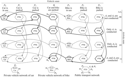
ATS aims at obtaining ATPs that optimize a certain objective. An ATP entails the sequence of activities and locations, transportation modes and routes, and parking locations for conducting a daily activity program (AP). ATS is considered as a path choice through networks of different states (Liao, Arentze, and Timmermans 2011, 2013). In a multi-state supernetwork, three states are distinguished:

1. Activity state: describing which activities have already been conducted.

2. Vehicle state: describing where the private vehicles (PVs) are, i.e. in use or parked somewhere.

3. Activity-vehicle state: the combination of activity and vehicle states.

The nodes in a multi-state supernetwork denote physical locations. Three types of links are defined:

1. Travel links: connecting different nodes representing the movement in a transportation network, staying in the same state.

2. Transition links: connecting the same nodes of different transportation modes (i.e. parking/picking-up a PV, boarding/alighting public transportation).

3. Transaction links: connecting the same nodes of different activity states representing the implementation of activities.

A multi-state supernetwork is illustrated in Figure 1 (undirected links are bi-directed). The private vehicle networks (PVNs) for PVs and public transportation networks (PTNs) for walking and public transit (PT) are copied for every possible activity-vehicle state. The vertices of PVNs and PTNs are home and activity and parking locations. Specifically, $A_1$and $A_2$ are two activities; each has one alternative location for simplicity; each row represents an activity state; $s_1$and $s_2$ denote the activity states of $A_1$and $A_2$ respectively (0: not conducted; 1: conducted). Car and bike are two private vehicles (PVs); columns $P_1$ & $P_2$ and $P_3$ & $P_4$ are the vehicle states where the car and bike can be parked respectively. All PVs must be parked when conducting activities. Columns $P_0$and $P_5$ are the vehicle states where car and bike are in use respectively. ${\text{H}}_0$ and ${\text{H}}_1$ are the home location at the start and end states of an AP. Any path from ${\text{H}}_0$ to ${\text{H}}_1$ represents a full ATP, potentially including multi-modal and multi-activity trip chaining. For example, the bold path represents an ATP, indicating an individual leaves home ($H_0$) by car, parks the car at $P_2$, travels through PTN to conduct $A_1$, returns home to switch to bike with parking at $P_4$ for conducting $A_2$, and finally returns home ($H_1$) with all PVs parked at home and all activities conducted.

Figure 1. Multi-state supernetwork representation (Liao 2016).

In the deterministic multi-state supernetwork, link attributes are deterministic. The disutility of a link can be defined in a state- and time-dependent way as (1) $\begin{array}{c}{d}_{isml}(t)=f({\mathit{\beta }}_{isml},{\mathit{X}}_{isml}(t))\end{array}$(1) where $d_{isml}(t)$ is the disutility of link $l$ at state $s$ with transportation mode $m$ at time $t$ for individual $i$. $f(\cdot )$ is a disutility function of link attributes, in which ${\mathit{X}}_{isml}(t)$ denotes a vector of static or time-dependent link attributes and ${\mathit{\beta }}_{isml}$ is a vector of disutility coefficients of link attributes. For the sake of simplicity, linear additive disutility functions are mostly assumed for travel, transition, and transaction links with waiting durations, but non-linear disutility functions are a more general functional form. A particular ATP is found by optimizing this function. Minimizing disutility (or generalized cost) is the most applied principle in the scheduling literature (Rasouli and Timmermans 2014). In case of minimizing the disutility, the objective of ATS is expressed as (2) $\begin{array}{c}min\{d({\lambda }_{{\text{H}}_0\to {\text{H}}_1})\},{\lambda }_{{\text{H}}_0\to {\text{H}}_1}\in PATH\end{array}$(2) where ${\lambda }_{{\text{H}}_0\to {\text{H}}_1}$ denotes an ATP from origin ${\text{H}}_0$ to destination ${\text{H}}_1$ in path space$PATH$ and $d({\lambda }_{{\text{H}}_0\to {\text{H}}_1})$ is the disutility of ${\lambda }_{{\text{H}}_0\to {\text{H}}_1}$.

An STD multi-state supernetwork, referred to as SNK, is constructed for an individual’s AP over an STD multi-modal transportation network by attaching stochasticity to the links. Let $SNK(\mathit{v},\mathit{l},\mathit{t})$ denote the STD multi-state supernetwork, where $\mathit{v}$ is the set of nodes, $\mathit{l}$ is the set of links, and $\mathit{t}$ is the set of discrete time intervals within a day. In SNK, the travel times on routes and durations for conducting activities are time-dependent random variables. Any path from ${\text{H}}_0$ to ${\text{H}}_1$ represents an ATP at a high level of detail with stochastic disutility, subject to time window constraints at some locations. The objective is to schedule an ATP under uncertainty. Alternative objectives in Equation (2) can be chosen. This study applies expected disutility minimization for illustration purposes only.

Notation List

The following notations are used in this study.

STD multi-state supernetwork

SNK	=	individual STD multi-state supernetwork
$\mathit{v}$,$\mathit{l}$,$\mathit{t}$	=	set of nodes, links, and time intervals within a day
$|\cdot |$	=	operator to calculate the number of elements in a set
$l$	=	link in SNK, $l\in \mathit{l}$
$t$	=	discrete time interval, $t\in \mathit{t}$
$s$	=	state in SNK
$m$	=	transportation mode
$i$	=	an individual (traveler)
${\text{H}}_0,{\text{H}}_1$	=	origin and destination nodes of daily ATPs
$\lambda$	=	path departing from the origin node ${\text{H}}_0$ and arriving at the current node

Stochastic route travel time and activity duration

$p$	=	route for a trip, $p\in \mathit{p}$, $\mathit{p}$ is the set of routes for all the trips in SNK
$X_{ip}(t)$	=	stochastic travel time of route $p$ at $t$ for individual $i$
$\alpha$, $o_{\alpha }$, $\mathit{\alpha }$	=	an activity, a location for the activity, and activity set, respectively, $\alpha \in \mathit{\alpha }$
$D_{i{o}_{\alpha }}(t)$	=	stochastic activity duration of conducting $\alpha$ at location $o_{\alpha }$ at $t$ for individual $i$

Support points

$n$, $n^{\mathrm{\prime }}$	=	$n$-th and $n^{\mathrm{\prime }}$-th time zone in the time zone set $\mathit{n}$, $n,n^{\mathrm{\prime }}=1,\dots |\mathit{n}|$.
$r$	=	support point covers all the time zones, $r\in \mathit{r}$
$p_r$	=	probability of support point$r$, $\sum _r{p}_r=1,r\in \mathit{r}$
${\rho }_n$	=	spatial correlation coefficient within time zone $n$
${\delta }_{n{n}^{\mathrm{\prime }}}$	=	temporal correlation coefficient between time zone $n$ and $n^{\mathrm{\prime }}$

Recursive formulations in SNK for ATS

$j,k$	=	nodes of SNK (locations of interest)
$t_j$	=	arrival time at node $j$
$d_{\lambda }(j,t_j,r)$	=	disutility of $\lambda$ arriving at node $j$ at $t_j$ at support point $r$
$x_{\lambda }(j,t_j,r)$	=	travel time of $\lambda$ arriving at node $j$ at $t_j$ at support point $r$
$c_{\lambda }(j,t_j,r)$	=	monetary expense of $\lambda$ arriving at node $j$ at $t_j$ at support point $r$
$z_{s{j}_{\alpha }}(t,D_{j_{\alpha }})$	=	disutility of conducting activity $\alpha$ at $j$ with start time $t$ and duration $D_{j_{\alpha }}$ at state $s$
$z_w(t,w)$	=	disutility of waiting at time $t$ with waiting duration $w$

Pathfinding algorithm

$\mathit{\lambda }$	=	set of non-dominated paths from ${\text{H}}_0$ to current node
${\mathcal{X}}_j$	=	set of pure paths from $H_0$ to $j$
${\mathit{V}}_j^{+1}$	=	set of successor nodes of node $j$

3. ATS approach

In this section, we propose an approach of individual ATS under time-dependent spatially and temporally correlated uncertainty, subject to a set of constraints. First, we provide general formulations of stochastic time-dependent travel times and activity durations based on an individual’s personalized STD multi-state supernetwork. Next, we discuss the generation of support points for representing the spatially and temporally correlated stochastic components and investigate the effectiveness of the proposed generation method. Finally, recursive formulations are suggested for path extension in a space–time multi-state supernetwork.

3.1. Stochastic route travel time and activity duration

Different from trip scheduling that usually focuses on unimodal trips in a short time period, ATS concerns a full AP of a longer time frame. Technically, finding the optimal ATPs in a large urban environment involving all choice facets and alternatives suffers from the curse of dimensionality. Liao, Arentze, and Timmermans (2011, 2013), therefore, developed a heuristic approach to select a small set of flexible activity locations that locally optimally connect the fixed locations such as home and workplace. With the pre-selection of locations, personalized multi-state supernetworks are constructed to delimit the action space.

Based on the constructed personalized multi-state supernetworks, it is assumed that the individual mainly concerns a few routes interconnecting relevant points of interest rather than every road segment or link of the routes. This assumption has a practical basis that only the known alternatives that satisfy an individual’s constraints and preferences form the choice set available for the individual in reality (Bovy 2009; Prato 2009). It is also supported by studies that considered travel time reliability of route rather than specific links (e.g. Tilahun and Levinson 2010). Following the same reasoning, it is assumed that an individual considers time-dependent route travel time and activity durations across multiple time zones that differentiate major travel periods of a day, since that they would not process the differences of the uncertainties at an excessive high time dimension. Given these assumptions, we formulate the stochastic travel times and activity durations for ATS below.

For the individual ATS, the stochasticity of the activity-travel choice facets needs to be considered given realistic assumptions in a time-dependent context. In an STD multi-state supernetwork, a trip is considered a part of a trip chain connecting the locations of interest. A route typically connects locations related to the AP (e.g. home, activity locations, and transportation mode transfer locations), using a certain transportation mode. Stochastic route travel time has the following characteristics:

1. the stochastic route travel time includes three components: free-flow travel time, stochastic route-specific travel time, and correlated travel time;

2. the time-invariant free-flow route travel time refers to the situation without uncertainty and congestion;

3. the stochastic route-specific travel time is due to the uncertainty related to the time of the day and route characteristics;

4. the correlated route travel time includes temporal and spatial correlations with other routes and activity durations.

The time-dependent stochastic route travel time is expressed as (3) $\begin{array}{c}{X}_{ip}(t)=x_{0ip}+X_{1ip}(t)+{\epsilon }_{i\overline{p}}(t)\end{array}$(3) where $X_{ip}(t)$ is the stochastic travel time of route $p$ ($p\in \mathit{p}$) at time $t$ of individual $i$, $x_{0ip}$ is the time-invariant free-flow travel time of $p$, $X_{1ip}(t)$ is the stochastically independent route-specific travel time of $p$ at $t$, and ${\epsilon }_{i\overline{p}}(t)$ is the correlated travel time component of $p$ at $t$ that captures the spatial and temporal dependencies with route travel times other than $p$ and activity durations at locations. The representation can be decomposed by discarding one or two components on the right-hand side (RHS) of Equation (3). In SNK, a trip may have multiple route alternatives. In the network modeling literature, a route set for a trip can be generated using path generation methods (e.g. Prato 2009; Wang et al. 2019).

In most ATS-related studies, travel time and activity duration have been treated largely in isolation (e.g. Fu and Lam 2014; Liao, Rasouli, and Timmermans 2014). However, traffic congestion close to activity locations may turn into delays in activity service times and hence activity duration (Jenelius 2012). Hence, we consider that stochastic travel time and activity duration may be correlated, despite not necessarily symmetrically. Specifically, stochastic activity duration has the following characteristics:

1. the stochastic activity duration includes three activity duration components: minimum duration, stochastic activity-specific duration, and correlated duration;

2. the minimum duration is time-invariant, dependent on activity type and activity location;

3. the stochastic activity-specific duration is due to the uncertainty related to the time of the day and the individual’s knowledge of location characteristics;

4. the correlated duration is due to the spatial and temporal correlations with travel times and activity durations at other locations.

The time-dependent stochastic activity duration under uncertainty is expressed as (4) $\begin{array}{c}{D}_{i{o}_{\alpha }}(t)=d_{0i{o}_{\alpha }}+D_{1i{o}_{\alpha }}(t)+{ϵ}_{i\overline{o_{\alpha }}}(t)\end{array}$(4) The three components on the RHS of Equation (4) correspond to the three components of the stochastic activity duration for conducting $\alpha$ at $t$ at activity location $o_{\alpha }$ by individual $i$, where $d_{0i{o}_{\alpha }}$ is the time-invariant minimum duration, $D_{1i{o}_{\alpha }}(t)$ is the stochastically independent activity-specific duration, and ${ϵ}_{i\overline{o_{\alpha }}}(t)$ is the correlated duration of conducting activity $\alpha$ at location $o_{\alpha }$. Likewise, Equation (4) can be simplified by ignoring one or two components on the RHS.

Formally, we suppose the ATS time frame is divided into a set $\mathit{n}$ of time zones. For any time interval $t$ within the n-th time zone, the travel times of all routes and activity durations of related activities are uncertain according to Equations (3, 4). Component ${\epsilon }_{i\overline{p}}(t)$ in $X_{ip}(t)$ is spatially mutually correlated with ${\epsilon }_{i\overline{p^{\mathrm{\prime }}}}(t)$ in $X_{i{p}^{\mathrm{\prime }}}(t)$ of another route $p^{\mathrm{\prime }}$ and ${ϵ}_{i\overline{o_{\alpha }}}(t)$ in $D_{i{o}_{\alpha }}(t)$; in addition, ${\epsilon }_{\overline{p}}(t)$ and ${\epsilon }_{\overline{p}}(t^{\mathrm{\prime }})$ are temporally correlated for $p$ between $t$ and $t^{\mathrm{\prime }}$ in time zone $n$ and $n^{\mathrm{\prime }}$ respectively, $n,n^{\mathrm{\prime }}\in \mathit{n}$; likewise, ${ϵ}_{i\overline{o_{\alpha }}}(t)$ and ${ϵ}_{i\overline{o_{\alpha }}}(t^{\mathrm{\prime }})$ are temporally correlated at $o_{\alpha }$ between the two time intervals.

3.2. Representation of stochasticity using support points

‘Support points’ are a set of representative points obtained by compacting a continuous distribution (Mak and Joseph 2018). Huang and Gao (2012) defined a support point as a distinct value (vector of values) that a discrete random variable (vector) can take and applied a set of support points of the joint probability mass function to represent correlated link travel times. For example, in a time-dependent network with two paths (links) over two time intervals, a support point with a certain probability consists of a vector of four distinct travel times. Thus far, applications of support points to trip scheduling involved a short time span (e.g. Huang and Gao 2012). When the time span is long, for example, covering a full-day as for ATS, a large set of support points may be necessary to cover all possible realizations of stochasticity. However, as for individual ATS, we use a limited set of representative support points to represent the stochasticity of a personalized STD multi-state supernetwork. Empirical evidence is provided by some studies to support the assumption of limited set of support points. Löhndorf (2016) presented an empirical analysis of using a small set of scenarios to approximate a continuous multivariate distribution. More methods that reduce the number of scenarios while retaining the quality of the stochasticity (in the forms of continuous or discrete distributions) can be found in stochastic programming (e.g. Dupačová, Gröwe-Kuska, and Römisch 2003; Rujeerapaiboon et al. 2018). It is believed that an individual possesses only a limited number of support points of a heavily reduced personalized network for daily ATS. Meanwhile, from the perspective of individual uncertainty, many previous studies (Miller 1956; Hogarth 1975; Smith, Benson, and Curley 1991) showed that humans are weak in perceiving the uncertainty and tend to simplify the distribution of the uncertain events to accommodate their limited cognitive ability, corresponding to the limited set of support points.

Let $r$ be a support point that covers the entire time frame $\mathit{t}$ with probability $p_r$, $r\in \mathit{r}$, a realization of all stochastic components in Equations (3, 4) for all the routes and related activities, satisfying $\sum _r{p}_r=1$. Each $r$ is associated with a vector of time-dependent route travel times and activity durations, corresponding to one space–time multi-state supernetwork. The stochasticity of the STD multi-state supernetwork with correlations among the stochastic components is fully expressed by support point set $\mathit{r}$.

We propose a method to generate a set of support points of STD route travel times and activity durations taking into account the spatial and temporal correlations. The method first constructs a correlation matrix involving the spatial and temporal correlations according to Equations (3, 4), then samples a large number of discrete points (e.g. 10⁶) from the truncated multivariate distribution ensuring that the stochastic travel times and activity durations are not lower than the free-flow travel times and minimum durations, and finally generates the representative support points using a generation method. The procedures of constructing the correlation matrix and the generation method are given below.

First, we create a $\omega \cdot |\mathit{n}|$ by $\omega \cdot |\mathit{n}|$ correlation coefficient matrix $\mathrm{\Sigma }$, where $\omega$ denotes the number of stochastic components of route travel times and activity durations according to Equations (3, 4) in SNK, which is equal to $(|\mathit{p}|+|\mathit{\alpha }|)$ when all correlated components for route travel time and activity duration are considered. $\mathit{\alpha }$ is the set of activities in AP and $|\cdot |$ defines the cardinality of a set.

1. For the spatial correlations within a time zone, the dimension of correlation matrix ${\mathrm{\Sigma }}_n(t)$ at time $t$ (${\mathrm{\Sigma }}_n$ for short) within time zone $n$ is $\omega$ by $\omega$. In the present case, a constant correlation structure with a specific coefficient value (Hardin, Garcia, and Golan 2013) is assumed for ${\mathrm{\Sigma }}_n$. The spatial correlation coefficient ${\rho }_n$ for each ${\mathrm{\Sigma }}_n$ is simply assumed to be the same, represented as $\rho$. More complex correlation structures can be estimated.

2. For the temporal correlations across time zones, correlation matrix $\mathrm{\Sigma }$ has blocks ${\mathrm{\Sigma }}_1$,${\mathrm{\Sigma }}_2$, … .,${\mathrm{\Sigma }}_{|\mathit{n}|}$ along the diagonal. The off-diagonal blocks refer to ‘inter-time zone’ correlation matrices, captured by correlation coefficients of the off-diagonal blocks. Let ${\mathrm{\Sigma }}_{n{n}^{\mathrm{\prime }}}$ be the correlation matrix between time zone $n$ and $n^{\mathrm{\prime }}$ with temporal correlation coefficient ${\delta }_{n{n}^{\mathrm{\prime }}}$. $\mathrm{\Sigma }$ is denoted as (5) $\begin{array}{c}\mathrm{\Sigma }=\left(\begin{array}{cc}\begin{array}{cc}{\mathrm{\Sigma }}_1& {\mathrm{\Sigma }}_{12}\\ {\mathrm{\Sigma }}_{21}& {\mathrm{\Sigma }}_2\end{array}& \begin{array}{cc}\cdots & {\mathrm{\Sigma }}_{1|\mathit{n}|}\\ \cdots & {\mathrm{\Sigma }}_{2|\mathit{n}|}\end{array}\\ \begin{array}{cc}⋮& ⋮\\ {\mathrm{\Sigma }}_{|\mathit{n}|1}& {\mathrm{\Sigma }}_{|\mathit{n}|2}\end{array}& \begin{array}{cc}\ddots & ⋮\\ \cdots & {\mathrm{\Sigma }}_{|\mathit{n}|}\end{array}\end{array}\right)\end{array}$(5)

3. $\mathrm{\Sigma }$ is positive semi-definite with ${\delta }_{n{n}^{\mathrm{\prime }}}$ satisfying $0\le {\delta }_{n{n}^{\mathrm{\prime }}}\le \rho$, assuming ${\delta }_{n{n}^{\mathrm{\prime }}}$ is the baseline for temporal correlation (see Hardin, Garcia, and Golan (2013) for more details). Given the variances of the stochastic components, a positive semi-definite covariance matrix is obtained.

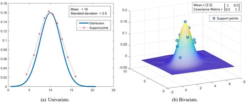
Next, given the constructed covariance matrix, we apply the K-means clustering algorithm (Dougherty, Kohavi, and Sahami 1995; Gupta, Mehrotra, and Mohan 2010) to generate support points by clustering the generated samples into a specific number of discrete data points. The centroid of one cluster is taken as the support point and the corresponding probability is determined by the density of the cluster. Huang and Gao (2012) sampled travel time vectors on stochastic links from a truncated multivariate normal distribution as support points and assigned an equal probability to each support point (i.e. 1/$|\mathit{r}|$, where $|\mathit{r}|$ is the number of support points; nevertheless, the details of generating the support points were not discussed). Conceptually, the clustering algorithm is appropriate by grouping data points of similar features (in terms of closeness) as distinct support points in the stochastic space, while data points in different supports have high dissimilarities. For example, Figure 2(a) and (b) show the generated support points of a univariate and a bivariate normal distribution respectively with $|\mathit{r}|=10$.

Figure 2. Examples of generated support points of normal distributions.

Tests on high-dimensional normal distributions output significantly different probability patterns from equal probabilities assigned to the generated support points with small sets of support points, while the differences are diminishing when the set of support points gets large. It signals that clustering method is likely to be more effective with a limited set of support points given that the stochastic space is usually uneven. The K-means clustering algorithm is easy to implement and becomes more stable with large samples. The average computational times for generating 10, 50, and 100 support points using K-means clustering method are 0.05, 0.15, and 0.18 s, respectively. Given the existence of multiple clustering algorithms (Saxena et al. 2017), future research should examine other alternative clustering algorithms or sampling methods, which may provide even better results.

3.3. Recursive formulations of path extension in SNK

Given the generated support points, we show the path extension for ATS in STD multi-state supernetwork with time window constraints. Denote $j$ as the last node of path ${\lambda }^{\mathrm{\prime }}$ and $t_j$ as the arrival time at $j$ at support point $r$. After extending ${\lambda }^{\mathrm{\prime }}$ with link $(j,k)$ to $\lambda$ in SNK, the arrival time at node $k$ on the newly extended $\lambda$ is updated as $t_k$. We illustrate the path extension considering time and monetary expenses as two disutility components. The time and monetary expenses of link $(j,k)$ at $t_j$ and support point $r$ are denoted by $X_{jk}^r(t_j)$ and $C_{jk}^r(t_j)$. Given $x_{{\lambda }^{\mathrm{\prime }}}(j,t_j,r)$ and $c_{{\lambda }^{\mathrm{\prime }}}(j,t_j,r)$ as the time and monetary expenses of ${\lambda }^{\mathrm{\prime }}$ at $t_j$ and $r$ respectively, the extensions of path time and monetary expenses are formulated as (6) $\begin{array}{rl}{x}_{\lambda }(k,t_k,r)& =x_{{\lambda }^{\mathrm{\prime }}}(j,t_j,r)+X_{jk}^r(t_j)\end{array}$(6) (7) $\begin{array}{rl}{c}_{\lambda }(k,t_k,r)& =c_{{\lambda }^{\mathrm{\prime }}}(j,t_j,r)+C_{jk}^r(t_j)\end{array}$(7) Denote $d_{{\lambda }^{\mathrm{\prime }}}(j,t_j,r)$ as the disutility of ${\lambda }^{\mathrm{\prime }}$ arriving at $j$ at $t_j$ and $\mathcal{F}(X_{jk}^r(t_j),C_{jk}^r(t_j))$ the disutility of $(j,k)$ at $r$. 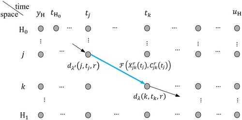With time window $[y_{\text{H}},u_{\text{H}}]$ for conducting all out-of-home activities, the recursive formulation on $d_{\lambda }(k,t_k,r)$ is represented as (8) $\begin{array}{r}{d}_{\lambda }(k,t_k,r)=\{\begin{array}{l}{d}_{{\lambda }^{\mathrm{\prime }}}(j,t_j,r)+F(X_{jk}^r(t_j),C_{jk}^r(t_j)),if{t}_k\le u_{\text{H}}\\ +\mathrm{\infty },if{t}_k>u_{\text{H}}\end{array}\end{array}$(8) Equation (8) is schematically shown in a space–time network (Figure 3). The blue link $(j,k)$ is regarded as a link in SNK with disutility $\mathcal{F}(X_{jk}^r(t_j),C_{jk}^r(t_j))$ at $t_j$ and $r$. After extending ${\lambda }^{\mathrm{\prime }}$ with $(j,k)$ to $\lambda$, $d_{\lambda }(k,t_k,r)$ is updated under time window constraints. In the course of path extension, different types of links are traversed, of which links are distinguished as non-activity (travel and transition) and activity (transaction) links. Recursive formulations of path time expense and disutility are given below.

Figure 3. Representation of a recursive formulation in a space-time network.

Non-activity links

SNK consists of multiple transportation modes and a travel link in SNK represents a route using a certain transportation mode connecting two locations of interest. For a change of transportation modes, parking or picking private vehicles (car or bike) and boarding or alighting the public transportation are represented as transition links. The arrival time at node $k$ of the extended $\lambda$ after traversing non-activity link $(j,k)$ is formulated as (9) $\begin{array}{r}\begin{array}{c}{t}_k=t_j+X_{jk}^r(t_j)\end{array}\end{array}$(9) The disutility of $\lambda$ arriving at $j$ and $r$ can be updated according to Equation (8).

Activity links with time window constraints

Traversing activity links may involve time window constraints at the activity locations. Suppose $[y_j,u_j]$ is the time window of location $j$ for activity $\alpha$. At $r$, the individual’s arrival time at $j$ for conducting $\alpha$ at state $s$ is $t_j$, and the arrival time at $j$ on $\lambda$ at state $s^{\mathrm{\prime }}$ after traversing a transaction link is $t_k$. The activity duration of conducting activity $\alpha$ at location $j$ at start time $t$ and support point $r$ is represented as $D_{j_{\alpha }}^r(t)$ according to Equation (4). If $t_j<y_j$, the individual has to wait at $j$ with duration $y_j-t_j$ and the start time of $\alpha$ is $y_j$; if $y_j\le t_j<u_j$, the individual could start to conduct $\alpha$ at $t_j$ immediately; if $t_j\ge u_j$, conducting $\alpha$ at $j$at $t_j$ is not allowed. $t_k$ is specified as (10) $\begin{array}{r}{t}_k=\{\begin{array}{ll}{y}_j+D_{j_{\alpha }}^r(y_j),& if{t}_j<y_j\\ t_j+D_{j_{\alpha }}^r(t_j),& if{y}_j\le t_j<u_j\\ +\mathrm{\infty },& if{t}_j\ge u_j\end{array}\end{array}$(10) According to Equation (8), $d_{\lambda }(k,t_k,r)$ is the disutility after extending ${\lambda }^{\mathrm{\prime }}$ with transaction link $(j,k)$ for conducting an activity at $r$. $j$ and $k$ represent the same activity location at different activity states. Denote the waiting duration by $w^r(t)$ ($w^r$ for short), the disutility of waiting by $z_w(t,w^r)$, and the disutility of conducting the activity with duration $D_{j_{\alpha }}^r(t)$ at $s$ by $z_{s{j}_{\alpha }}(t,D_{j_{\alpha }}^r(t))$. Respecting time window constraints, $d_{\lambda }(k,t_k,r)$ is formulated as (11) $\begin{array}{r}{d}_{\lambda }\left(k,t_k,r\right)=\left\{\begin{array}{ll}{d}_{{\lambda }^{\mathrm{\prime }}}\left(j,t_j,r\right)+z_w\left(t_j,w^r\right)+z_{s{j}_{\alpha }}\left(y_j,D_{j_{\alpha }}^r\left(y_j\right)\right),& \text{if}{t}_j<y_j\text{ and }{t}_k\le u_j\\ d_{{\lambda }^{\mathrm{\prime }}}\left(j,t_j,r\right)+z_{s{j}_{\alpha }}\left(t_j,D_{j_{\alpha }}^r\left(t_j\right)\right),& \text{if }{y}_j\le t_j<u_j\text{ and }{t}_k\le u_j\\ +\mathrm{\infty },& \text{if }{t}_j\ge u_j\text{ or }{t}_k>u_j\end{array}\right.\end{array}$(11) $z_{s{j}_{\alpha }}(t,D_{j_{\alpha }}^r(t))$ is a start time and duration combined disutility function, which can be formulated in additive form as (12) $\begin{array}{r}\begin{array}{c}{z}_{s{j}_{\alpha }}(t,D_{j_{\alpha }}^r(t))=g_{s{j}_{\alpha }}(t,D_{j_{\alpha }}^r(t),{\beta }_t)+h_{s{j}_{\alpha }}(t,D_{j_{\alpha }}^r(t),{\beta }_c)\end{array}\end{array}$(12) where $g_{s{j}_{\alpha }}(t,D_{j_{\alpha }}^r(t),{\beta }_t)$ is the disutility function of activity duration at location $j$ at state $s$ with start time $t$ and duration $D_{j_{\alpha }}^r(t)$. $h_{s{j}_{\alpha }}(t,D_{j_{\alpha }}^r(t),{\beta }_c)$ is the disutility function of the monetary expense of conducting the activity. ${\beta }_t$ and ${\beta }_c$ are the individual’s disutility coefficients of time and monetary expenses respectively.

The above path extension process stops when path $\lambda$ reaches H₁, at which an ATP is completed and the ATP disutility is obtained.

4. Algorithm

The classic label-setting shortest path algorithm (Dijkstra 1959) has been adapted for finding the optimal paths in various contexts (e.g. Miller-Hooks and Mahmassani 2000; Dean 2004). In STD networks, Bellman’s principle of optimality tends to be violated, and thus the standard label-setting algorithm may not be applicable to ATS in STD multi-state supernetworks. Considering complete dependencies, Huang and Gao (2012) designed an exact label-correcting algorithm to find the optimal path with minimum expected disutility (MED), which maintains a non-dominated path set over space $\mathrm{\Omega }=\{(t,r)|t\in \mathit{t},r\in \mathit{r}\}$ for each node, instead of only keeping the paths with MED for each time $t$ in the space–time network. Following Huang and Gao (2012), we adopt a similar dominance rule in SNK. For each arrival node $k$ with arrival time $t_k$, the dominance of paths is defined as follows.

Definition 1 Dominance: A path $\lambda$ from ${\text{H}}_0$ to $k$ is non-dominated in $\mathrm{\Omega }$ if and only if no other path $\overline{\lambda }$ between the same OD pair such that (13) $\begin{array}{r}\begin{array}{c}{d}_{\overline{\lambda }}(k,t_k,r)\le d_{\lambda }(k,t_k,r),\mathrm{\forall }(t_k,r)\in \mathrm{\Omega }\end{array}\end{array}$(13) and the equation sign does not apply to all conditions.

Given non-dominated path set $\mathit{\lambda }$ from ${\text{H}}_0$ to $k$ with arrival time $t_k$, the optimal path depends on the objective. For illustration, we consider the objective is to minimize the expected disutility. Synthesizing Equations (8), (11) and (12), a linear additive form is assumed for the disutility function as (14) $\begin{array}{r}\begin{array}{c}{d}_{\lambda }(k,t_k,r)={\beta }_t\cdot x_{\lambda }(k,t_k,r)+{\beta }_c\cdot c_{\lambda }(k,t_k,r)\end{array}\end{array}$(14) where $x_{\lambda }(k,t_k,r)$ and $c_{\lambda }(k,t_k,r)$ are the time and monetary expenses of path $\lambda$ with arrival time $t_k$ at $r$, ${\beta }_t$ and ${\beta }_c$ are the individual parameters. In applications, the simple function can be replaced by an estimated (non)-linear multi-attribute function. Given the disutility of each non-dominated path $\lambda \in \mathit{\lambda }$, the expected disutility of $\lambda$ with arrival time $t_k$ is given as (15) $\begin{array}{r}\begin{array}{c}{e}_{\lambda }(k,t_k)=\sum _r{p}_r\cdot d_{\lambda }(k,t_k,r)\end{array}\end{array}$(15) Huang and Gao (2012) suggested a label-correcting algorithm in a time-expanded network to find a non-dominated path set. The algorithm is based on a concept of pure paths, which form a set of non-dominated paths that satisfy the Bellman principle. A path is pure if itself and all its sub-paths are non-dominated; otherwise, it is a mixed path. The pure paths are checked at any node and mixed non-dominated paths are deleted from the solution set before finding the optimal path.

We apply the label correcting algorithm of path extension to find all pure paths from ${\text{H}}_0$ to ${\text{H}}_1$ in SNK with MED. In the procedure, a pure path set ${\mathcal{X}}_j$ is maintained for node $j$; a node-path pair $⟨j,{\lambda }^{\mathrm{\prime }}⟩$ is selected at each iteration from the scan list for extending ${\lambda }^{\mathrm{\prime }}$ by traversing link $(j,k)$ to reach node $k$, selected from the successor nodes set ${\mathit{V}}_j^{+1}$, ${\lambda }^{\mathrm{\prime }}\in {\mathcal{X}}_j$. The acyclicity of the newly extended path is checked by backtracking the path to check if node $k$ is on the sub-path. If $\lambda$ doesn’t contain cycles, given any departure time $t_j$, $x_{\lambda }(k,t_k,r)$, $c_{\lambda }(k,t_k,r)$ and $d_{\lambda }(k,t_k,r)$ are updated.

Different departure times from predecessor node $j$ may reach node $k$ at the same arrival time $t_k$. On the other hand, not every possible arrival time within the time window can be realized in the time-expanded non-FIFO (first-in-first-out) supernetwork. The following steps are implemented before checking path dominance: (1) if $t_k$ is a realized time interval following $\lambda$, label $d_{\lambda }(k,t_k,r)$ is checked and updated with the least disutility; the corresponding departure time $t_j$, $x_{\lambda }(k,t_k,r)$ and $c_{\lambda }(k,t_k,r)$ are corrected accordingly; (2) for every unrevealed arrival time of node $k$ at $r$, the disutility label is corrected through a waiting link from an earlier revealed arrival time at $k$. The supplement of unrealized arrival times of node $k$ at $r$ reduce the size of non-dominated paths set; otherwise, the non-dominated paths set ${\mathcal{X}}_k$ becomes large if arrival times in the time-expanded supernetwork are sparsely filled according to Definition 1.

The dominance between $\lambda$ and paths in ${\mathcal{X}}_k$, containing only pure paths as the mixed paths are already removed, is checked according to the dominance rule (Definition 1). The label $⟨k,\lambda ⟩$ is added to ${\mathcal{X}}_k$ and the scanning list if $\lambda$ is not dominated. The algorithm stops when no node-path pair is in the scanning list. The scheduled ATPs of MED is obtained considering the pure paths at all possible arrival times and support points. The departure and arrival times at each node can be obtained by backtracking the optimal ATPs. The pseudo-code of the label-correcting algorithm is given below.

The time complexity of the proposed algorithm is analyzed as follows. Suppose $|\mathit{v}|$ and $|\mathit{l}|$ are the numbers of nodes and links in the personalized multi-state supernetwork. $|P|$ is the maximum number of generated non-dominated paths at a node, which may increase exponentially in size. Let $|\mathit{t}|$ and $|\mathit{r}|$ denote the numbers of discrete time intervals and support points. As the path extension and the dominance-checking are conducted for all arrival times and support points at each node, the path extension requires runtime $O(|P||\mathit{t}||\mathit{r}|)$; the procedure of checking dominance runs in time $O({|P|}^2|\mathit{t}||\mathit{r}|)$, which has a higher order than $O(|P||\mathit{t}||\mathit{r}|)$. The label-correcting algorithm finds the shortest path after at most $|\mathit{v}|-1$ passes of the full supernetwork. Therefore, the time complexity of the algorithm is $O({|P|}^2|\mathit{t}||\mathit{r}||\mathit{v}||\mathit{l}|)$. Although the algorithm has an exponential time complexity over the generated paths, it is applicable since that the ATS runs with a limited set of support points over small personalized networks. Thus, computation time is not a main source of concern for applications.

5. Examples

To illustrate the suggested approach for ATS, this section presents an example of a typical daily AP. The approach is executed using Matlab R2019a on a PC with Windows 10 using Intel Core i7-9750H CPU @ 2.60 GHz, 16.00GB RAM.

5.1. Setup

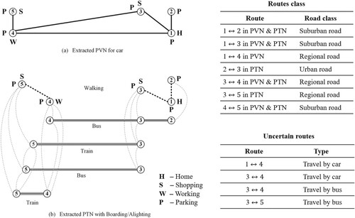
The daily AP and personalized networks are extracted from Liao, Rasouli, and Timmermans (2014). We consider the case in which the car is the only private mode in the PVN with 5 parking locations (P) and two public transportation modes, including bus and train in the PTN. Figure 4 represents the PVN and PTN as bi-directed graphs. The ATS time frame (6:00–20:00) distinguishes peak hours (7:00–9:00 and 17:00–19:00) and non-peak hours (other timeslots). We set 60 min per time zone during peak hours and each of three continuous timeslots in non-peak hours, making 7 time zones in total. The AP includes two activities and three activity locations, working (at node 4, W) and shopping (at nodes 3 or 5, S) with time windows [8:00, 18:00], [7:00, 18:00], and [8:00, 19:00] respectively. Node 1 is home with out-of-home time window [6:00, 20:00]. The multi-state supernetwork has 6 vehicle states and 4 activity states. Thus, there are 120 nodes, 430 links for all the departure times in the STD multi-state supernetwork. The routes with stochastic travel times are shown at the right-bottom of Figure 4 and other route travel times are assumed deterministic.

Figure 4. PVN and PTN.

The stochastic components of route travel times and activity durations are sampled from a truncated multivariate Gaussian distribution. The covariance matrices are constructed with different levels of spatial and temporal correlations (see section 3.2). We set values of 0.8, 0.5, and 0.2 for spatial correlation coefficient $\rho$ between two stochastic components within each time zone and for temporal correlation coefficient ${\delta }_{n{n}^{\mathrm{\prime }}}$ between every two time zones to represent high, medium, and low levels respectively. The K-means clustering algorithm is applied to generate the support points. The stochastic travel times and activity durations are shown in Table 2.

Table 2. Activity-travel time uncertainty (min).

			Time distribution
ID	Type	Route/Location	non-peak	peak-1	peak-2
1	Travel by car	1 $\leftrightarrow$ 4	(30, 5^2)	(37, 6^2)	(40, 7^2)
2	Travel by car	3 $\leftrightarrow$ 4	(28, 5^2)	(34, 6^2)	(37, 7^2)
3	Travel by bus	3 $\leftrightarrow$ 4	(32, 3^2)	(35, 4^2)	(35, 4^2)
4	Travel by bus	3 $\leftrightarrow$ 5	(30, 3^2)	(33, 4^2)	(33, 4^2)
5	Shopping	3	(20, 3^2)	(25, 3^2)	(25, 3^2)
6	Shopping	5	(22, 3^2)	(28, 5^2)	(28, 5^2)
7	Working	4	(15, 5^2)	(15, 5^2)	(15, 5^2)

The monetary expense is assumed to be linearly related with the time expense for travel, transition, and transaction links. To highlight the impact of spatial and temporal correlations, we adopt a simplified form of Equation (12) of activity disutility, formulated as a linear function of start time and activity duration. The related parameters are given in Table 3. We apply linear multi-attributes disutility functions with time and monetary expenses (Equation (14)) for all the links in the STD multi-state supernetwork. The parameters of time expense and monetary expense are set to 0.05 units of disutility per min and 0.1 units of disutility per € respectively.

Table 3. Monetary expense parameters.

Travel links	road class	Constant	Coefficient of time (min)
Car	Regional	0	0.1
	Suburban	0	0.12
	Urban	0	0.15
		Constant	Coefficient of length (km)
Bus		0.5	0.05
Train		0.5	0.05
Transaction links		Constant	Coefficient of time (min)
Shopping		5	0.5
Working		0	0

The headways of buses and trains are set as 7 min in peak-hours and 15 min in non-peak hours. The time expense parameters of the disutility function for taking the bus and the train are set to 0.055 units of disutility per min during peak-hours, reflecting the increasing discomfort of taking PT during peak hours as compared to non-peak hours. It takes 3 min to park the car and 1 min for boarding and alighting PT and picking up the car. Earlier arrival at activity locations and PT stations will cause waiting, waiting time punishment is considered. The parameters of waiting time including the waiting for time window and PT are set to 0.025 units of disutility per min. The departure times of PT vehicles from the starting stations are assumed to follow the timetable, but the arrival times at other stations are uncertain because of the stochastic route travel times. Considering the delayed arrivals, the PT vehicles have to adjust departure times with the same dwelling times at the PT stops/stations.

5.2. Results

Based on the above settings, the label-correcting algorithm finds the scheduled ATPs under MED. The algorithm is executed with different ${\delta }_{n{n}^{\mathrm{\prime }}}$ (levels of temporal correlation) and $\rho$ (levels of spatial correlation). For illustration, 10 support points are generated according to the method proposed in Section 3.2. Common ATPs that are scheduled in a series of tests are summarized in Table 4. The average running time is 0.52 s. Tests are conducted for different settings to illustrate the effects of spatial and temporal correlations on scheduled ATPs.

Table 4. Scheduled ATPs under MED in all the tests.

$\lambda$	Type	ATPs under MED
${\lambda }_1$	PVN	1 – car – 4 – work at 4 – car – 3 – shop at 3 – car – 1
${\lambda }_2$	PVN + PTN	1 – car – 3 – bus – 4 – work at 4 – train – 5 – shop at 5 – train – 3 – car - 1
${\lambda }_3$	PVN + PTN	1 – car – 3 – train – 5 – train – 4 – work at 4 – train – 5 – shop at 5 – train – 3 – car - 1
${\lambda }_4$	PVN + PTN	1 – car – 3 – shop at 3 – train – 5 – train – 4 – work at 4 – train – 5 – train – 3 – car - 1
${\lambda }_5$	PVN + PTN	1 – car – 3 – shop at 3 – bus – 4 – work at 4 – train – 5 – train – 3 – car - 1

Test 1: Effects of spatial correlation

The stochasticity of the individual STD multi-state supernetwork is set based on Table 2. Given different spatial correlation coefficient $\rho$ and a fixed temporal correlation coefficient as 0.2, the results of the scheduled ATPs are displayed in Table 5. The scheduled ATPs are shown in Figure 5, which entail the choice of transportation modes, routes, activity locations, activity sequence, and the departure/arrival times at locations. Since the departure/arrival time at each location varies with different support points, we show departure/arrival time ranges across all the support points in Figure 5 and other figures below.

Table 5. Scheduled ATPs with different $\rho$.

$\rho$	${\delta }_{n{n}^{\mathrm{\prime }}}$	Non-dominated Paths number	Optimal Label $(\lambda ,e_{\lambda }(H_1,t_{H_1}))$	Departure times in $\mathit{r}$	Arrival times	Activity sequence
0.2	0.2	40	(${\lambda }_1$, 32.04)	[7:13, 7:45]	17:26	W first, S at 3
0.5		29	(${\lambda }_2$, 32.38)	[7:33, 7:54]	17:51	W first, S at 5
0.8		49	(${\lambda }_3$, 32.41)	[7:26, 7:40]	17:37	W first, S at 5

Figure 5. Scheduled ATPs with ${\delta }_{n{n}^{\mathrm{\prime }}}=0.2$.

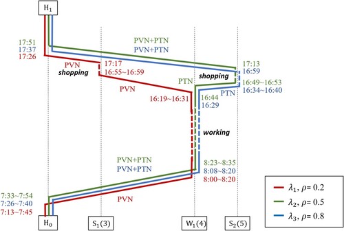
Given ${\delta }_{n{n}^{\mathrm{\prime }}}$=0.2, different ATPs are obtained for different degrees of spatial correlation coefficient $\rho$. When spatial correlation is low ($\rho$=0.2), the stochasticity of route travel times and activity durations are less influenced by each other in each time zone, and the scheduled ATP ${\lambda }_1$ involves going to work by car during morning peak hours and driving for shopping at node 3 during the evening peak hours, although the variance of traveling by car is high. When the spatial correlation increases ($\rho$=0.5), the stochastic travel times and activity durations are spatially more correlated. ${\lambda }_2$ suggests taking car through a route with a deterministic travel time and transferring to bus with a lower variance for work during morning peak hours, then going shopping by train and driving home. When the spatial correlation is high ($\rho$=0.8), the schedule involves taking the train through routes with deterministic travel times for working and shopping to avoid taking the transportation mode and routes with higher variances in any time zone.

The switches of transportation modes and routes in the scheduled ATPs illustrate the effects of spatial correlation on scheduled ATPs. The MED of the scheduled ATPs increases with increasing $\rho$ because the stochastic components more likely have larger values with higher spatial dependency in every time zone. The departure and arrival times at each location of the scheduled ATPs differ. Hence, the individual is suggested to depart from home earlier when taking ${\lambda }_1$ involving only PVN other than PVN + PTN of ${\lambda }_2$ and ${\lambda }_3$. For all scheduled ATPs, the optimal activity sequence is working prior to shopping. Shopping at location 3 is optimal when only taking car, while shopping at location 5 is more favorable when taking multimodal.

Test 2: Effects of temporal correlation

For this test, the spatial correlation coefficient is fixed as 0.8 and temporal correlation coefficient ${\delta }_{n{n}^{\mathrm{\prime }}}$ is systematically varied. Table 6 shows the results. The optimal schedules are illustrated in Figure 6.

Figure 6. Scheduled ATPs with $\rho =0.8$.

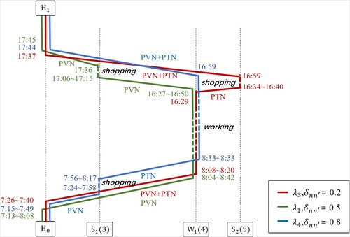
Table 6. Scheduled ATPs with different ${\delta }_{n{n}^{\mathrm{\prime }}}$.

$\rho$	${\delta }_{n{n}^{\mathrm{\prime }}}$	Non-dominated Paths number	Optimal Label $(\lambda ,e_{\lambda }(H_1,t_{H_1}))$	Departure times in $\mathit{r}$	Arrival times	Activity sequence
0.8	0.2	49	(${\lambda }_3$, 32.41)	[7:26, 7:40]	17:37	W first, S at 5
	0.5	47	(${\lambda }_1$, 32.57)	[7:13, 8:08]	17:45	W first, S at 3
	0.8	57	(${\lambda }_4$, 32.69)	[7:15, 7:49]	17:44	S at 3 first, W

When the temporal correlation is low (${\delta }_{n{n}^{\mathrm{\prime }}}$=0.2), the optimal ATP ${\lambda }_3$ suggests working first and then shopping at node 5 with a longer duration. When the temporal correlation increases (${\delta }_{n{n}^{\mathrm{\prime }}}$=0.5), the individual is suggested to depart early during morning peak hours by car. As route travel times and shopping durations are more correlated, the optimal ATP suggests shopping at location 3 with a shorter duration and lower variance than that at location 5 in the evening peak hours. When the temporal correlation is high (${\delta }_{n{n}^{\mathrm{\prime }}}$=0.8), the stochastic travel times and activity durations are highly correlated within and between time zones. To avoid congestion and crowdedness and longer shopping duration, which implies that shopping may not be completed within the time window, the optimal ATP ${\lambda }_4$ suggests shopping at location 3 before working and taking the PVN + PTN combination for traveling.

The MED of the scheduled ATPs increases with increasing ${\delta }_{n{n}^{\mathrm{\prime }}}$ since each stochastic component tends to have increasingly larger values across time zones during the day. The departure time windows of ATPs ${\lambda }_1$ and ${\lambda }_4$ are expanded compared with ${\lambda }_3$ since the uncertainty of the departure or arrival times increases with increasing correlations between the time zones.

Test 3: Effect of heterogeneous beliefs of uncertainty

Test 3 considers the ATS with a heterogeneous traveler, assuming that individual 2 holds different beliefs of uncertainty from individual 1 that PV is relatively more unreliable compared to tests 1 and 2, by increasing the variance of route travel times by car. The variances of route travel times by car for the three time zones in Table 2 are set to 6², 7², 8² respectively. After generating a new set of 10 support points, the results of scheduled ATPs are shown in Table 7 under different combinations of spatial and temporal correlations.

Table 7. Scheduled ATPs with different $\rho$ and ${\delta }_{n{n}^{\mathrm{\prime }}}$.

$\rho$	${\delta }_{n{n}^{\mathrm{\prime }}}$	Non-dominated Paths number	Optimal Label $(\lambda ,e_{\lambda }(H_1,t_{H_1}))$	Departure times in $\mathit{r}$	Arrival times	Activity sequence
0.2	0.2	43	(${\lambda }_3$, 32.38)	7:40, 7:47	17:51	W first, S at 5
0.8		59	(${\lambda }_3$, 32.41)	[7:26, 7:40]	17:37	W first, S at 5
0.8	0.2	59	(${\lambda }_3$, 32.41)	[7:26, 7:40]	17:37	W first, S at 5
	0.8	59	(${\lambda }_4$, 32.69)	[7:23, 7:49]	17:44	S at 3 first, W

Given the higher travel time variances associated with traveling by car, the combination of car and train is recommended for individual 2. ${\lambda }_3$ is the scheduled ATP for ${\delta }_{n{n}^{\mathrm{\prime }}}=0.2$ and $\rho =0.2$, which is different from ATP ${\lambda }_1$ in tests 1. When the spatial correlation increases ($\rho =0.8$) or the temporal correlation increases (${\delta }_{n{n}^{\mathrm{\prime }}}=0.8$), the route travel times and activity durations are more spatially and correlated, resulting in an increasing MED. The number of non-dominated paths increases compared with the results of tests 1 and 2, reflecting the effects of variability and correlations on the optimally scheduled ATPs.

Test 4: Effects of number of support points

With the clustering method for generating the support points, we test how many support points would be needed to generate stable results. The results in Table 8 shows that for 10 support points, stability for ATP ${\lambda }_4$ is already achieved with the spatial and temporal correlations are at a high level ($\rho =0.8$, ${\delta }_{n{n}^{\mathrm{\prime }}}=0.8$). From $|\mathit{r}|=20$ to 60, the stability of the results further increases for more correlation scenarios. For $|\mathit{r}|$ larger than 70, the scheduled ATPs are stable under all the correlation combinations. The results of the test indicate that a limited number of support points seems sufficient to achieve stability in the optimal schedules. In tests 1–3, we use 10 support points based on the consideration that individual consideration sets tend to be limited even in large networks.

Table 8. Scheduled ATPs with different $\rho$ and ${\delta }_{n{n}^{\mathrm{\prime }}}$ of different $|\mathit{r}|$.

	Optimal label $(\lambda ,e_{\lambda }(H_1,t_{H_1}))$ with correlation combination $(\rho ,{\delta }_{n{n}^{\mathrm{\prime }}})$
$|\mathit{r}|$	$(0.2,0.2)$	$(0.5,0.2)$	$(0.8,0.2)$	$(0.8,0.5)$	$(0.8,0.8)$
10	(${\lambda }_1$, 32.04)	(${\lambda }_2$, 32.38)	(${\lambda }_3$, 32.41)	(${\lambda }_1$, 32.57)	(${\mathit{\lambda }}_4$, 32.69)
20	(${\mathit{\lambda }}_3$, 32.40)	(${\lambda }_3$, 32.39)	(${\lambda }_1$, 32.50)	(${\lambda }_1$, 32.58)	(${\mathit{\lambda }}_4$,32.69)
30	(${\mathit{\lambda }}_3$, 32.41)	(${\lambda }_3$, 32.40)	(${\lambda }_1$, 32.56)	(${\mathit{\lambda }}_4$, 32.68)	(${\mathit{\lambda }}_4$,32.68)
40	(${\mathit{\lambda }}_3$, 32.41)	(${\lambda }_3$, 32.41)	(${\mathit{\lambda }}_5$, 32.68)	(${\mathit{\lambda }}_4$, 32.69)	(${\mathit{\lambda }}_4$,32.69)
50	(${\mathit{\lambda }}_3$, 32.40)	(${\lambda }_1$, 32.57)	(${\mathit{\lambda }}_5$, 32.67)	(${\mathit{\lambda }}_4$, 32.68)	(${\mathit{\lambda }}_4$,32.69)
60	(${\mathit{\lambda }}_3$, 32.41)	(${\lambda }_1$, 32.56)	(${\mathit{\lambda }}_5$, 32.68)	(${\mathit{\lambda }}_4$, 32.68)	(${\mathit{\lambda }}_4$,32.67)
70	(${\mathit{\lambda }}_3$, 32.40)	(${\mathit{\lambda }}_5$, 32.68)	(${\mathit{\lambda }}_5$, 32.68)	(${\mathit{\lambda }}_4$, 32.69)	(${\mathit{\lambda }}_4$,32.69)
80	(${\mathit{\lambda }}_3$, 32.41)	(${\mathit{\lambda }}_5$, 32.66)	(${\mathit{\lambda }}_5$, 32.66)	(${\mathit{\lambda }}_4$, 32.68)	(${\mathit{\lambda }}_4$,32.69)
90	(${\mathit{\lambda }}_3$, 32.40)	(${\mathit{\lambda }}_5$, 32.67)	(${\mathit{\lambda }}_5$, 32.67)	(${\mathit{\lambda }}_4$, 32.69)	(${\mathit{\lambda }}_4$,32.69)
100	(${\mathit{\lambda }}_3$, 32.40)	(${\mathit{\lambda }}_5$, 32.68)	(${\mathit{\lambda }}_5$, 32.67)	(${\mathit{\lambda }}_4$, 32.68)	(${\mathit{\lambda }}_4$,32.68)

The spatial and temporal correlation coefficients reflect the degree of dependencies among the travel and activity components within a time zone and between different time zones. The variance of an ATP’s time expense or disutility increases with increasing link covariance, given the assumption that the link monetary expense is linearly related with link time expense in the examples (a link here corresponds to travel, transition, or transaction link in the multi-state supernetwork).

For the effects of spatial correlations, when the spatial correlation is low (e.g. $\rho =0.2$), the ATP extension process considers less the chosen links’ variances within each time zone to obtain the minimum disutility. With an increase in the spatial correlation (e.g. from $\rho =0.2$ to 0.5 or 0.8), the ATP extension would choose connected links with lower variances. The results in Table 5 and Figure 5 reflect such choice adaptations given 10 support points. When the spatial correlation is low ($\rho =0.2$), travel by car, despite with higher variances, is preferred in the scheduled ATP regardless of time zones. With an increase in spatial correlation ($\rho =0.5$), when the travel link (link 3–4) and activity link (working at node 4) are traversed within the same time zone, travel by bus with lower variances is chosen instead of by car. When $\rho =0.8$, travel by the combination of car and train is chosen to avoid larger variances because travel by train has deterministic travel times.

For the effects of temporal correlations, the links are more correlated with higher temporal correlations across the whole time frame, given a spatial correlation coefficient. The ATP’s variance increases with respect to the variances of spatially correlated links within each time zone as well as the link variances from any other time zones, given a level of temporal correlation. When the temporal correlation is high (e.g. ${\delta }_{n{n}^{\mathrm{\prime }}}=0.8$), conducting flexible activities at activity locations with shorter durations and lower variances is preferred, comparing to lower temporal correlations (e.g. ${\delta }_{n{n}^{\mathrm{\prime }}}=0.2$). Table 6 and Figure 6 show the changes in activity locations and activity sequence with varied temporal correlations. Adaptation is made from shopping at node 5 with a longer duration and a higher variance provided with a low temporal correlation (${\delta }_{n{n}^{\mathrm{\prime }}}=0.2$) to shopping at node 3 with a relatively shorter duration and a lower variance provided with a high temporal correlation (${\delta }_{n{n}^{\mathrm{\prime }}}=0.8$). To ensure the activities are conducted within the time windows, shopping before working is preferred when the temporal correlation is high.

The results of tests 1 and 2 illustrate that the choices are adapted across different facets of an ATP given different combinations of spatial and temporal correlations. For example, compared with the scheduled ATP in the case with low correlations ($\rho =0.2$ and ${\delta }_{n{n}^{\mathrm{\prime }}}=0.2$), different route, transportation mode, and activity sequence are scheduled with the combination of relatively high correlations ($\rho =0.8$ and ${\delta }_{n{n}^{\mathrm{\prime }}}=0.8$). Moreover, we use the normalized Levenshtein distance to measure the difference of the multi-dimensional ATPs based on the activity type, location, and transportation mode of the scheduled ATPs (Joh, Arentze, and Timmermans 2008). Given different pairs of spatial correlation coefficients (e.g. $\rho =0.2$ and $\rho =0.8$ as a pair) with the same temporal correlation, the average normalized Levenshtein distance between every two scheduled ATPs is 0.46, indicating that the degree of dissimilarity of the ATPs affected by spatial correlation is approximately 46 percent. Similarly, the measure equals 0.44 given different temporal correlation coefficient pairs with the same spatial correlation. For capturing the extent to which ATP would differ having heterogeneous travelers in the network, a second individual with different beliefs of uncertainty (reflected in different sets of support points) is assumed in test 3. The highest normalized Levenshtein distance is 0.67 when the transportation mode choice of the scheduled ATPs is changed given large differences of travel time variances between PV and PT.

The above tests demonstrate the applicability of the suggested ATS approach for a typical daily AP. The uncertainty and stochastic dependencies are considered in the proposed algorithm. As indicated, the spatial and temporal correlations have effects on optimally scheduled ATPs. Meanwhile, the scheduled ATPs are affected by different beliefs of uncertainty with heterogeneous travelers. A limited number of support points are exemplified to be sufficient to capture the stochasticity and achieve the stability of the optimal ATPs.

6. Conclusions and future work

Extant work on ATS based on multi-state supernetworks has mostly relied on a deterministic representation. Some explorative seminal work has been conducted on a stochastic representation of travel times, but this work has been formal in nature, assuming independence. This paper extends this body of knowledge in a number of aspects. First, the stochasticity is extended to also include the multiple activity durations, conditional on time windows. Second, the assumption of independence is replaced with allowing for spatial and temporal correlations among uncertain activity-travel components. These extensions require other algorithms to find the optimal schedule. In this study, representative support points are generated using a clustering algorithm. Non-dominated time-dependent ATPs are obtained by recursive formulations through the STD multi-state supernetwork. The extension is the first one in the literature that incorporates spatial and temporal correlations for individual ATS and innovatively combines the concepts of support point and personalized multi-state supernetwork. Given the pervasiveness of uncertainties for daily activity-travel, this extension is necessary and serves as a departure point for many planned works.

A series of numerical experiments has been carried out for different settings to verify the performance of the proposed ATS model. The results of tests 1 and 2 indicate that the optimally scheduled ATPs indeed are affected by spatial and temporal correlations among the stochastic travel times and activity durations. The ATPs are adapted to avoid the increasing of the variance of the ATP’s disutility in the event of high levels of spatial and temporal correlations respectively. The results of test 3 demonstrate that the proposed model is sensitive to traveler heterogeneity, reflected in the differences in the optimal schedules. All changes can be directly interpreted in the changes in the scheduled ATPs. Also, we explored the effect of the number of support points on the stability of the optimally scheduled ATP. The results of all the tests indicate that the stochasticity of individual STD multi-state supernetworks and the correlations in space and time can be sufficiently captured by the proposed model and the generated support points. The proposed ATS model can be applied for a personalized recommendation system provided with dynamically updated personalized parameters. For applications in travel demand forecasting, the model can be extended by adding unobserved error terms and more realistic choice-making mechanisms under uncertainty.

Nevertheless, several issues are worth further investigation. First, since the applicability of the ATS model strongly depends on the accurate representation of AP-specific personalized multi-state supernetworks, the estimation of the objective function and the demarcation of individual consideration sets needs further exploration. With the increasing availability of revealed data (e.g. GPS trajectories), it seems feasible to derive validated representations of individual STD multi-state supernetworks. Second, we suggested using the K-means clustering algorithm as a distribution discretization method to generate a specific number of support points. This specific method was chosen for its theoretical properties that seem to be appropriate for the problem at hand. However, future work may explore other clustering algorithms and particularly more efficient space covering sampling methods in terms of their relative accuracy and efficacy. Third, the proposed ATS model finds optimal ATPs at the individual level, ignoring task and resource allocation, joint activities, and joint (partial) travel arrangements. Extensions to the household and meeting group level are relevant and timely. Finally, although the label-correcting algorithm with the recursive formulations is a rigorous way of generating non-dominated ATPs considering full dependencies, the algorithm may need to be revisited for higher efficiency in different circumstances.

Disclosure statement

No potential conflict of interest was reported by the author(s).

Acknowledgements

The first author is grateful to the financial support by the China Scholarship Council (CSC). This study is partly supported by the Dutch Research Council (NWO, project no. 438-18-401).

Correction Statement

This article has been republished with minor changes. These changes do not impact the academic content of the article.

Additional information

Funding

This work was supported by China Scholarship Council (CSC): [Grant Number [2017]3109]; Nederlandse Organisatie voor Wetenschappelijk Onderzoek: [Grant Number 438-18-401].

References

- Arentze, T. A., and H. J. P. Timmermans. 2004. “Multistate Supernetwork Approach to Modelling Multi-Activity, Multimodal Trip Chains.” International Journal of Geographical Information Science 18 (7): 631–651.
- Bhat, C. R., and F. S. Koppelman. 1999. “Activity-based Modeling of Travel Demand.” Handbook of Transportation Science, Springer, Boston, MA 35–61.
- Bovy, P. H. 2009. “On Modelling Route Choice Sets in Transportation Networks: A Synthesis.” Transport Reviews 29 (1): 43–68.
- Bowman, J. L., and M. E. Ben-Akiva. 2001. “Activity-based Disaggregate Travel Demand Model System with Activity Schedules.” Transportation Research Part A: Policy and Practice 35 (1): 1–28.
- Chen, B. Y., W. H. K. Lam, Q. Li, A. Sumalee, and K. Yan. 2013. “Shortest Path Finding Problem in Stochastic Time-Dependent Road Networks with Stochastic First-in-First-out Property.” IEEE Transactions on Intelligent Transportation Systems 14 (4): 1907–1917.
- Chen, B. Y., W. H. K. Lam, A. Sumalee, and Z. L. Li. 2012. “Reliable Shortest Path Finding in Stochastic Networks with Spatial Correlated Link Travel Times.” International Journal of Geographical Information Science 26 (2): 365–386.
- Dean, B. C. 2004. “Shortest Paths in FIFO Time-dependent Networks: Theory and Algorithms.” Rapport technique, Massachusetts Institute of Technology.
- Dijkstra, E. W. 1959. “A Note on two Problems in Connection with Graphs.” Numerische Mathematik 1 (1): 269–271.
- Dougherty, J., R. Kohavi, and M. Sahami. 1995. “Supervised and Unsupervised Discretization of Continuous Features.” Machine learning proceedings 1995. Morgan Kaufmann 194–202.
- Dupačová, J., N. Gröwe-Kuska, and W. Römisch. 2003. “Scenario Reduction in Stochastic Programming.” Mathematical Programming 95 (3): 493–511.
- Fan, Y. Y., R. E. Kalaba, and J. E. Moore, II. 2005. “Shortest Paths in Stochastic Networks with Correlated Link Costs.” Computers & Mathematics with Applications 49 (9–10): 1549–1564.
- Fu, X., and W. H. K. Lam. 2014. “A Network Equilibrium Approach for Modelling Activity-Travel Pattern Scheduling Problems in Multi-Modal Transit Networks with Uncertainty.” Transportation 41 (1): 37–55.
- Fu, X., W. H. K. Lam, and B. Y. Chen. 2014. “A Reliability-Based Traffic Assignment Model for Multi-Modal Transport Network Under Demand Uncertainty.” Journal of Advanced Transportation 48 (1): 66–85.
- Gan, L. P., and W. Recker. 2008. “A Mathematical Programming Formulation of the Household Activity Rescheduling Problem.” Transportation Research Part B: Methodological 42 (6): 571–606.
- Gan, L. P., and W. Recker. 2013. “Stochastic Preplanned Household Activity Pattern Problem with Uncertain Activity Participation (SHAPP).” Transportation Science 47 (3): 439–454.
- Gao, S., and I. Chabini. 2006. “Optimal Routing Policy Problems in Stochastic Time-Dependent Networks.” Transportation Research Part B: Methodological 40: 93–122.
- Gupta, A., K. G. Mehrotra, and C. Mohan. 2010. “A Clustering-Based Discretization for Supervised Learning.” Statistics & Probability Letters 80 (9–10): 816–824.
- Hardin, J., S. R. Garcia, and D. Golan. 2013. “A Method for Generating Realistic Correlation Matrices.” The Annals of Applied Statistics 7 (3): 1733–1762.
- Hogarth, R. M. 1975. “Cognitive Processes and the Assessment of Subjective Probability Distributions.” Journal of the American Statistical Association 70 (350): 271–289.
- Huang, H., and S. Gao. 2012. “Optimal Paths in Dynamic Networks with Dependent Random Link Travel Times.” Transportation Research Part B: Methodological 46 (5): 579–598.
- Huang, H., and S. Gao. 2018. “Trajectory-adaptive Routing in Dynamic Networks with Dependent Random Link Travel Times.” Transportation Science 52 (1): 102–117.
- Jenelius, E. 2012. “The Value of Travel Time Variability with Trip Chains, Flexible Scheduling and Correlated Travel Times.” Transportation Research Part B: Methodological 46 (6): 762–780.
- Joh, C. H., T. A. Arentze, and H. J. P. Timmermans. 2008. “DANA: Dissimilarity Analysis of Activity travel Patterns.” Eindhoven, the Netherlands.
- Li, Q., F. Liao, H. J. P. Timmermans, and J. Zhou. 2016. “A User Equilibrium Model for Combined Activity–Travel Choice Under Prospect Theoretical Mechanisms of Decision-Making Under Uncertainty.” Transportmetrica A: Transport Science 12 (7): 629–649.
- Liao, F. 2016. “Modeling Duration Choice in Space–Time Multi-State Supernetworks for Individual Activity-Travel Scheduling.” Transportation Research Part C: Emerging Technologies 69: 16–35.
- Liao, F., T. A. Arentze, and H. J. P. Timmermans. 2010. “Supernetwork Approach for Multimodal and Multiactivity Travel Planning.” Transportation Research Record 2175 (1): 38–46.
- Liao, F., T. A. Arentze, and H. J. P. Timmermans. 2011. “Constructing Personalized Transportation Networks in Multi-State Supernetworks: a Heuristic Approach.” International Journal of Geographical Information Science 25 (11): 1885–1903.
- Liao, F., T. A. Arentze, and H. J. P. Timmermans. 2012. “Supernetwork Approach for Modeling Traveler Response to Park-and-Ride.” Transportation Research Record 2323 (1): 10–17.
- Liao, F., T. A. Arentze, and H. J. P. Timmermans. 2013. “Incorporating Space–Time Constraints and Activity-Travel Time Profiles in a Multi-State Supernetwork Approach to Individual Activity-Travel Scheduling.” Transportation Research Part B: Methodological 55: 41–58.
- Liao, F., S. Rasouli, and H. J. P. Timmermans. 2014. “Incorporating Activity-Travel Time Uncertainty and Stochastic Space–Time Prisms in Multistate Supernetworks for Activity-Travel Scheduling.” International Journal of Geographical Information Science 28 (5): 928–945.
- Löhndorf, N. 2016. “An Empirical Analysis of Scenario Generation Methods for Stochastic Optimization.” European Journal of Operational Research 255 (1): 121–132.
- Mak, S., and V. R. Joseph. 2018. “Support Points.” The Annals of Statistics 46 (6A): 2562–2592.
- Miller-Hooks, E. D., and H. S. Mahmassani. 2000. “Least Expected Time Paths in Stochastic, Time-Varying Transportation Networks.” Transportation Science 34 (2): 198–215.
- Miller, G. A. 1956. “The Magical Number Seven, Plus or Minus two: Some Limits on our Capacity for Processing Information.” Psychological Review 63 (2): 81.
- Nie, Y. M., and X. Wu. 2009a. “Reliable a Priori Shortest Path Problem with Limited Spatial and Temporal Dependencies.” In Transportation and Traffic Theory 2009: Golden Jubilee, 169–195.
- Nie, Y. M., and X. Wu. 2009b. “Shortest Path Problem Considering on-Time Arrival Probability.” Transportation Research Part B: Methodological 43 (6): 597–613.
- Prato, C. G. 2009. “Route Choice Modeling: Past, Present and Future Research Directions.” Journal of Choice Modelling 2 (1): 65–100.
- Rasouli, S., and H. J. P. Timmermans. 2014. “Activity-based Models of Travel Demand: Promises, Progress and Prospects.” International Journal of Urban Sciences 18 (1): 31–60.
- Rujeerapaiboon, N., K. Schindler, D. Kuhn, and W. Wiesemann. 2018. “Scenario Reduction Revisited: Fundamental Limits and Guarantees.” Mathematical Programming, 1–36.
- Saxena, A., M. Prasad, A. Gupta, N. Bharill, O. P. Patel, A. Tiwari, E. M. Joo, W. P. Ding, and C. T. Lin. 2017. “A Review of Clustering Techniques and Developments.” Neurocomputing 267: 664–681.
- Shahabi, M., A. Unnikrishnan, and S. D. Boyles. 2013. “An Outer Approximation Algorithm for the Robust Shortest Path Problem.” Transportation Research Part E: Logistics and Transportation Review 58: 52–66.
- Smith, G. F., P. G. Benson, and S. P. Curley. 1991. “Belief, Knowledge, and Uncertainty: A Cognitive Perspective on Subjective Probability.” Organizational Behavior and Human Decision Processes 48 (2): 291–321.
- Tilahun, N. Y., and D. M. Levinson. 2010. “A Moment of Time: Reliability in Route Choice Using Stated Preference.” Journal of Intelligent Transportation Systems 14 (3): 179–187.
- Waller, S. T., and A. K. Ziliaskopoulos. 2002. “On the Online Shortest Path Problem with Limited arc Cost Dependencies.” Networks: An International Journal 40 (4): 216–227.
- Wang, D., F. Liao, Z. Gao, and H. J. P. Timmermans. 2019. “Tolerance-based Strategies for Extending the Column Generation Algorithm to the Bounded Rational Dynamic User Equilibrium Problem.” Transportation Research Part B: Methodological 119: 102–121.
- Xing, T., and X. Zhou. 2011. “Finding the Most Reliable Path with and Without Link Travel Time Correlation: A Lagrangian Substitution Based Approach.” Transportation Research Part B: Methodological 45 (10): 1660–1679.
- Yang, L., and X. Zhou. 2014. “Constraint Reformulation and a Lagrangian Relaxation-Based Solution Algorithm for a Least Expected Time Path Problem.” Transportation Research Part B: Methodological 59: 22–44.
- Zockaie, A., H. S. Mahmassani, and Y. M. Nie. 2016. “Path Finding in Stochastic Time Varying Networks with Spatial and Temporal Correlations for Heterogeneous Travelers.” Transportation Research Record: Journal of the Transportation Research Board 2567 (1): 105–113.
- Zockaie, A., Y. M. Nie, X. Wu, and H. S. Mahmassani. 2013. “Impacts of Correlations on Reliable Shortest Path Finding.” Transportation Research Record: Journal of the Transportation Research Board 2334 (1): 1–9.